Abstract
The Qilian Mountain Area (QMA) serves as a crucial ecological barrier and strategic water conservation zone in China. Recent years have seen heightened social attention to environmental issues within the QMA, underscoring the need for accurate and continuous land cover maps to support ecological monitoring, analysis, and forecasting. This paper presents the QMA_LC30 dataset, which includes 9 land cover categories and spans the period from 1990 to 2020, with updates every 5 years. The dataset primarily utilizes 30 m Landsat series data and features: 1) High precision, achieved through a geographical division and hierarchical classification decision tree approach, complemented by visual interpretation. 2) Robust consistency, ensured by a change detection method based on a benchmark map. The QMA_LC30 dataset undergoes rigorous accuracy validation, achieving an overall accuracy of over 0.92 for all 7 periods of land cover maps. Compared to GlobeLand30, ESA WorldCover, ESRI 2020 Land Cover, FROM_GLC30, and GLC_FCS30, QMA_LC30 demonstrates the highest consistency with remote sensing images.
Subject terms: Environmental impact, Hydrology
Background & Summary
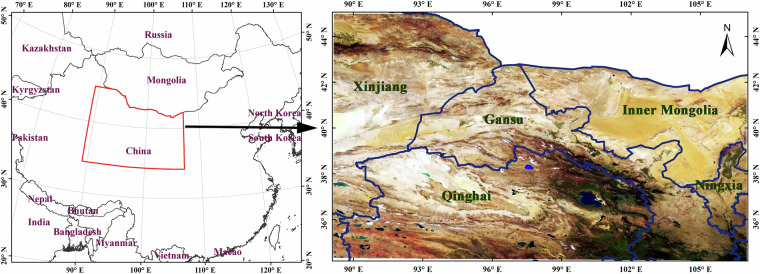
The Qilian Mountain Area (QMA), showed in Fig. 1, is located at the convergence of the Qinghai-Tibet Plateau, Mongolian Plateau, and Loess Plateau. This region serves as a vital ecological security buffer and a key area for water conservation in China, with a diverse biodiversity. Moreover, it is a significant central hub within the “Silk Road Economic Belt” and “the Third Pole”. Spanning approximately 1,548,000 km2 (extending from 89°–107° E, 34°–45° N), the QMA accounts for one-sixth of China’s total land area.
Fig. 1.
Location of the QLMR (left) and its true color Landsat image (right). The boundaries of provinces are also plotted out.
In recent years, the QMA has experienced significant ecological damage due to the combined effects of climate change and human activities. Major concerns include disruptions caused by extensive mineral resource development, haphazard hydropower and water resource utilization, and tourism activities that neglects the reserve’s core ecological functions. These issues have severely undermined the overall and long-term ecological and barrier functions of the QMA. The Chinese government has demonstrated strong commitment to addressing these ecological challenges, issuing critical directives and comments on multiple occasions. In June 2017, the General Office of the Central Committee of the Communist Party of China and the General Office of the State Council issued a “Notice on the Supervision and Handling of Ecological and Environmental Issues in the Qilian Mountain National Nature Reserve in Gansu and Their Lessons Learned,” identifying critical ecological and environmental issues in the Gansu section of the Qilian Mountain National Nature Reserve. Chinese President Xi Jinping has visited the Qilian Mountains multiple times to monitor and commend progress in ecological environment restoration. However, the lack of crucial data complicates understanding the complex interactions between climate change, human activities, and ecological systems, impeding the effective implementation of ecological governance practices.
Land cover classification products are invaluable in depicting the distribution of both natural and human-made surface features like vegetation, soil, water bodies, and built structures. These products are crucial for improving ecological, hydrological, and atmospheric models, and are widely used in research areas such as global climate change, earth system modeling, natural resource management, food security, and conservation biology1–4. Long-term land cover classification datasets are essential for monitoring the impacts of human activities on land cover dynamics and for guiding informed ecological governance decisions.
Several datasets covering the QMA are available through the National Tibetan Plateau Third Pole Environment Data Center (TPDC) website (https://data.tpdc.ac.cn/en/), as detailed in Table 1. Despite their accessibility, these products have limitations for continuous and long-term monitoring:
Limited spatial coverage. Many products focus only on the Heihe River Basin or specific key areas within the QMA, rather than covering the entire study area.
Temporal gaps. Existing products are restricted to specific year(s) and lacking continuity over time, requiring validation for consistency across different periods and hindering their use for sustained long-term monitoring.
Table 1.
Land cover products published on TPDC.
| No. | Product Name | Time Period | Spatial Extent | Spatial Resolution* | Declared Overall Accuracy | Literature or Data Source |
|---|---|---|---|---|---|---|
| 1 | MICLCover land cover map of the Heihe river basin (2000) | 2000 | Heihe River Basin (96.1°–104.2° E, 37.7°–43.3° N) | 1 km | 82.94% | Ran et al.23,24 |
| 2 | Land use/Land cover data of the Heihe River Basin | 1980s、2000 | Heihe River Basin (96.1°–104.2° E, 37.7°–43.3° N) | 30 m | — | Liu et al.25 Wang et al.26,27 Hu et al.28 |
| 3 | HiWATER: Land cover map of the Heihe River Basin | 2011–2015, monthly | Heihe River Basin (96.1°–104.2° E, 37.7°–43.3° N) | 30 m | 92.19% | Zhong et al.2,4,29 |
| 4 | The land cover/use data in key areas of the Qilian Mountain (2018). | 2018 | Key area of QMA (94°–102° E, 36°–39° N) | 2 m | — | Qi et al.30 |
| 5 | Land use/land cover dataset of Zhangye city in 2005 | 2005 | Zhangye city (96.1°–104.2° E, 37.7°–43.3° N) | 30 m | — | Yan31 |
| 6 | Landuse/landcover data of Zhangye city (2007) | 2007 | Zhangye city (96.1°–104.2° E, 37.7°–43.3° N) | 30 m | — | Hu et al.28,32,33 |
| 7 | Landcover dataset of the Shulehe River Basin (2000) | 2000 | Shulehe (92°–100° E, 37.88°–43.12° N) | 30 m | — | Liu et al.34 |
| 8 | Landuse/Landcover data of the QinghaiLake River Basin (2000) | 2000 | QinghaiLake (97.56°–101.45° E, 36.17°–38.42° N) | 30 m | — | Liu et al.35 |
*The measurement units employed in these published products vary. Products 2, 7, and 8 are designated by ‘scale’ (e.g., 1:100,000), whereas others utilize ‘spatial resolution’. To streamline comparison, all measurements have been standardized to ‘spatial resolution’.
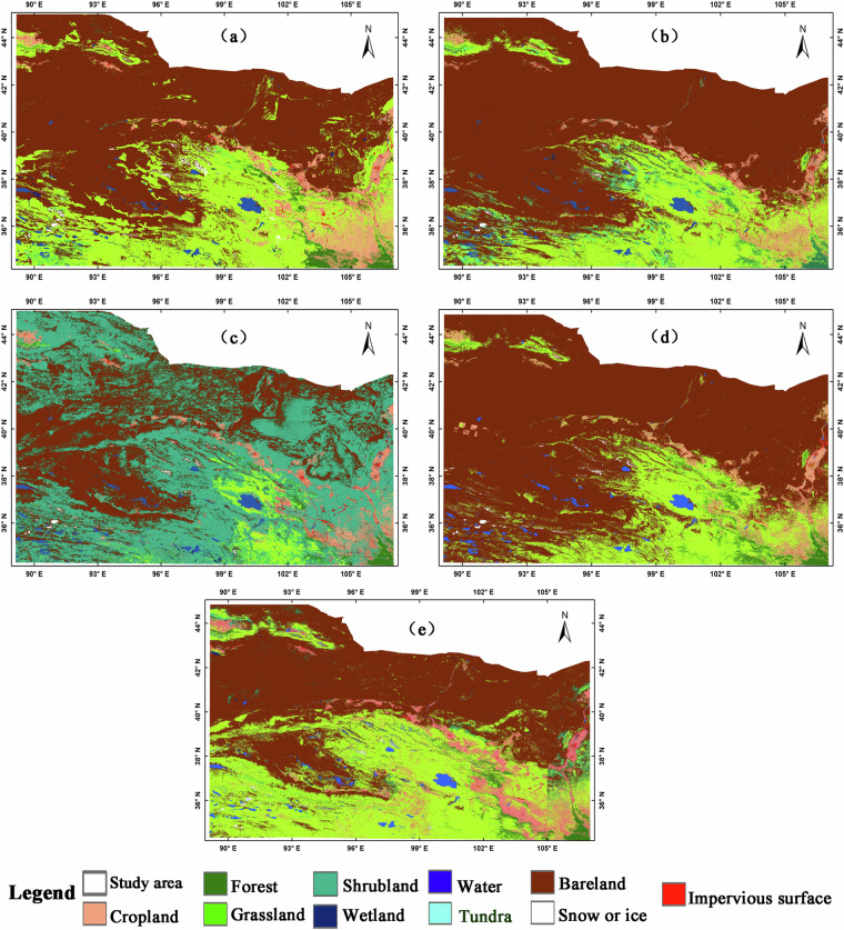
In recent years, several global medium and high-resolution land cover classification products have emerged, driven by advancements in remote sensing and big data technology. Notable examples include GlobeLand305, FROM_GLC30/FROM_GLC106,7, GLC_FCS308, ESA WorldCover9, and ESRI 2020 Land Cover10. Figure 2 shows the spatial distribution of these products in 2020 across the QMA, after standardizing the classification system and spatial resolution. While these products exhibit a similar overall pattern, there is significant inconsistency, especially in grassland, shrubland, and bare land. Moreover, most of these products cover only one or two time periods, making them insufficient for long-term change analysis. Therefore, there is an urgent need for a comprehensive set of medium and high-resolution land cover classification products that offer strong consistency and precision over extended time frames, specifically for the QMA.
Fig. 2.
Five land cover products covered QMA in 2020 after unifying classification system and spatial resolution. (a) GlobeLand30. (b) ESA WorldCover. (c) ESRI 2020 Land Cover. (d) FROM_GLC30. (e) GLC_FCS30.
This paper presents the QMA_LC30 dataset, which details land cover changes in the QMA at 5-year intervals from 1990 to 2020. The dataset is generated using a geographical division and hierarchical classification approach, combined with a change detection method based on long-term 30 m Landsat series data. To demonstrate the product’s advantages, conducted a comprehensive verification process, including accuracy assessments of land cover maps for each period and analysis of changes from 1990 to 2020. Additionally, the dataset is extensively compared with other land cover products to highlight its distinctive strengths.
Methods
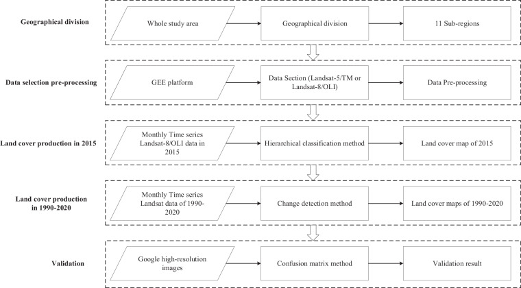
Figure 3 illustrates the workflow for generating the land cover product for the QMA, encompassing five key stages: geographical division, data selection and preprocessing, land cover production for 2015 using time series analysis and hierarchical classification, land cover production from 1990 to 2020 through change detection method, and comprehensive validation procedures.
Fig. 3.
Procedure of generating the QMA_LC30.
Geographical division
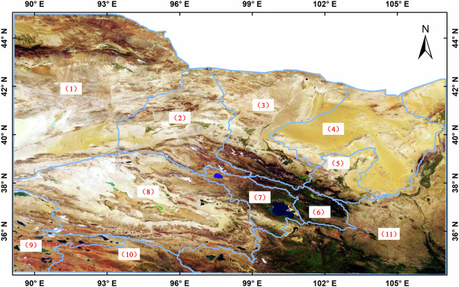
Given the siginificant geomorphic diversity, extensive coverage, and fragmented surface types within the study area, a strategic geographical division is crucial to ensure classification accuracy. The study employs a division method that partitions the large-scale region into 11 smaller sub-regions (see Fig. 4), which include: (1) the Kumutag Desert region, (2) the Shule River Basin region, (3) the Heihe River Basin region, (4) the Hexi Desert region, (5) the Shiyang River Basin region, (6) the Huangshui River Basin region, (7) the Qinghai Lake Water System region, (8) the Western Qaidam Basin region, (9) the Qiangtang Plateau region, (10) the Tongtian River Basin region, and (11) the Lanzhou Xiaheyan region. This geographical division strategy simplifies the extraction rules for land cover types and enhances the overall classification accuracy.
Fig. 4.
11 sub regions through geographical division of the QMA. (1) Kumutag Desert region, (2) Shule River Basin region, (3) Heihe River Basin region, (4) Hexi Desert region, (5) Shiyang River Basin region, (6) Huangshui River Basin region, (7) Qinghai Lake Water System region, (8) Western Qaidam Basin region, (9) Qiangtang Plateau region, (10) Tongtian River Basin region, and (11) Lanzhou Xiaheyan region.
Data selection pre-processing
GEE is a cloud-based platform provided by Google for online computation, analysis, processing and visualization of a vast array of global geoscientific data, including remote sensing imagery, climate and meteorological data, geophysical data, and various ready-to-use products11,12. GEE facilitates rapid batch processing of large image datasets and supports operations such as calculating indices like NDVI13, predicting crop yields14–16, monitoring land changes17–19, and more.
The primary data used in this study are sourced from the Landsat series of satellites, accessible via the GEE platform. The Landsat program, a collaborative effort between the United States Geological Survey (USGS) and the National Aeronautics and Space Administration (NASA), has been pivotal in Earth observation since 1972. While Landsat-5 operated from 1984 to 2013, Landsat-8 was launched in 2013 and continus to function. The combination of the Thematic Mapper (TM) on Landsat-5 and the Operational Land Imager (OLI) on Landsat-8 enables continuous Earth monitoring.
This study primarily utilizes surface reflectance data from Landsat-5/TM (1990–2010) and Landsat-8/OLI (2015–2020) in a time series framework, encompassing a total of 12,315 scenes, including 1478 scenes in 1990, 1409 scenes in 1995, 1742 scenes in 2000, 1709 scenes in 2005, 1671 scenes in 2010, 2175 scenes in 2015 and 2131 scenes in 2020. Additionally, auxiliary classification data are incorporated, including Digital Elevation Models (DEMs) from the Shuttle Radar Topography Mission (SRTM), Nighttime Lights Time Series from the Defense Meteorological Program Operational Line-Scan System (DMSP-OLS), Visible Infrared Imaging Radiometer Suite data from the Suomi NPP satellite (NPP-VIIRS), Sentinel-1/2 data, and high-resolution imagery from Google Earth. Table 2 provides the detailed information of these data and their usage.
Table 2.
Detailed information and usage of data used in this study.
| Spatial resolution | Temporal resolution | Spectral bands used | Time range | Usage in the mapping | |
|---|---|---|---|---|---|
| Landsat-5/TM | 30 m | 16 days | VNIR and SWIR bands | 1989–2013 | Provides time series data for classification |
| Landsat-8/OLI | 30 m | 16 days | VNIR and SWIR bands | 2014-present | Provides time series data for classification |
| SRTM | 90 m | N/A | N/A | N/A | Extract types related to terrain as auxiliary data, like water, snow or ice, and cropland |
| DMSP-OLS | 1000 m | 1 day | N/A | 1992–2013 | Extract impervious surfaces as auxiliary data |
| NPP-VIIRS | 500 m | 1 day | N/A | 2014-present | Extract impervious surfaces as auxiliary data |
| Sentinel-1 | 10 m | 12/6 days | VV and VH bands | 2014-present | Extract impervious surfaces as auxiliary data |
| Sentinel-2 | 10 m | 5 days | VNIR and SWIR bands | 2015-present | Used as a supplementary data source for time series data after 2015 |
| Google Earth imagery | Up to 1 m | N/A | N/A | N/A | Used as classification reference, and validation sample selection |
Data pre-processing involves several key steps, including cloud removal, image clipping and compositing, and the calculation of normalized indices such as NDVI, MNDWI. The Landsat L2A product offers a ‘QA_PIXEL’ band that containing quality attributes for each pixel, enabling the removal of pixels affected by cloud and cloud shadows. Image clipping is carried out using sub-region vectors and the ‘clip’ function within the GEE platform.
To capture the dynamic changes in land cover throughout a year, monthly composites of multispectral bands and NDVI are generated. The compositing process organizes all band values within a month after cloud removal, with the median value as the composite band value. The GEE’s ‘normalizedDifference’ function is used to compute normalized indices, specifically NDVI and MNDWI. NDVI is derived from the red and near-infrared bands, while MNDWI is calculated using the green and shortwave infrared bands. For monthly NDVI composites, the maximum value composite method is selected to minimize cloud and shadow interference.
Following data pre-processing, a series of twelve images containing multispectral bands and NDVI for each month of the target year in the QMA are generated, forming a comprehensive time series. However, it is important to note that due to data quality and observational limitations, obtaining a complete set of twelve monthly composite images/NDVIs for every year may not always be feasible. In such cases, images from adjacent years are used as supplementary data. MNDWI is calculated using synthesized images from rainy season months to ensure maximum water coverage can be captured.
Land cover production in 2015
The classification system outlined in Table 3, based on GlobeLand305, omits the “Tundra” category due to its infrequent occurrence in the QMA. As depicted in Fig. 3, the 2015 land cover map serves as a benchmark for generating maps of other time periods. Given the QMA’s vast scope and extensive data, this technical framework ensures consistency across land cover maps over multiple periods, facilitating continuous monitoring and analysis of land surface changes.
Table 3.
Classification system for the QMA_LC30.
| Code | Class | Content |
|---|---|---|
| 1 | Cropland | Land used for crop cultivation includes paddy fields, irrigated and rainfed drylands, vegetable field, forage planting areas, greenhouse land, and areas primarily used for crop cultivation with occasional fruit trees and other economically valuable arbor trees. It also encompasses shrub-type economic crop areas such as tea gardens and coffee plantations. |
| 2 | Forest | Land covered by arbor trees with a canopy cover exceeding 30%, including deciduous broad-leaved forests, evergreen broad-leaved forests, deciduous coniferous forests, evergreen coniferous forests, and mixed forests. It also includes open forest land with a canopy cover ranging from 10% to 30%. |
| 3 | Grassland | Land covered by natural herbaceous vegetation with over 10% coverage, including grasslands, meadows, savannas, desert grasslands, and urban artificial grasslands, among others. |
| 4 | Shrubland | Land covered by shrubs with over 30% shrub cover, including mountain shrublands, deciduous and evergreen shrublands, as well as desert shrublands with over 10% cover in desert regions. |
| 5 | Wetland | Land situated at the interface between terrestrial and aquatic environments, characterized by shallow water or saturated soil, often supporting marsh or aquatic vegetation. This includes inland marshes, lake marshes, river floodplain wetlands, forest/shrub wetlands, peat marshes, mangroves, salt marshes, and similar areas. |
| 6 | Water | Land covered by bodies of liquid water, including rivers, lakes, reservoirs, ponds, and similar features. |
| 7 | Impervious surface | Land altered by human activities, including urban and rural areas, industrial and mining sites, and transportation infrastructure. This excludes contiguous green spaces and water bodies within developed areas. |
| 8 | Bareland | Land with vegetation cover of less than 10%, including deserts, sandy areas, gravel fields, bare rock, and saline-alkali land. |
| 9 | Snow or ice | Land covered by permanent snow, glaciers, and ice sheets, including high mountain glaciers and polar ice sheets. |
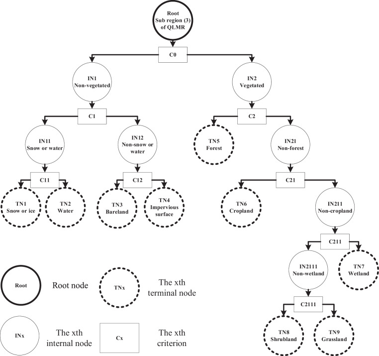
To map the 2015 land cover, a hierarchical classification decision tree approach is employed. This method involves constructing a tree structure with a root node, internal nodes (INs), and terminal nodes (TNs). The root node represents the entire classification domain and all relevant data, while each IN defines rules to partition nodes into distinct segments. The TNs, or leaves, represent the final classification categories determined by the associated INs.
The hierarchical decision tree method is noted for its simplicity, efficiency, and flexibility, making it particularly well-suited for applications requiring high classification accuracy in areas with complex surface characteristics. However, it does have a limitation: the need for substantial prior knowledge to establish node rules, which can slightly reduce classification efficiency.
In this study, distinct decision trees are constructed for each of the 11 sub-regions within the QMA. Consider the decision tree for sub-region (3) shown in Fig. 5. The root node includes the complete monthly synthesized time series of Landsat images and NDVI, supplemented by MNDWI for rainy season amalgamation. Although Landsat-8/OLI has a 16-day revisit cycle, resulting in fewer than two observations per month, the QMA’s arid and semi-arid climate typically minimizes cloud interference, allowing for near-complete and clear observations each month. In cases of missing data, Landsat-8/OLI images from adjacent years can be used as supplemental sources.
Fig. 5.
An example of a hierarchical classification decision tree of sub region (3).
Each decision tree features internal nodes (INs) equipped with rules for hierarchical identification of various land cover types. These rules are based on prior knowledge of vegetation phenology, spatial texture, elevation distribution, spectral features, and temporal change dynamics of each land cover category. Expert-defined thresholds for each IN’s rules are established through accumulated experience. Terminal nodes (TNs) represent the 9 target land cover types outlined in Table 3 and derived from their parent INs, as detailed in Table 4.
Table 4.
Rules of every node in the hierarchical classification decision tree of sub region (3).
| Criterion code | Input data | Rules | Outputs when rules are met | Outputs when rules not met |
|---|---|---|---|---|
| C0 | Landsat time series data | Max(NDVI) ≤ 0.2 | Non-vegetated | Vegetated |
| C1 | MNDWI in summer season (May., Jun., Jul., Aug., and Sep.) from Landsat data | MNDWIsum ≥ 0 | Snow or water | Non-snow or water |
| C11 | Synthetic image in summer season from Landsat data,and SRTM data | ρ(blue) ≥ 0.1 | Snow or ice | Water |
| DEM ≥ 3500 | ||||
| C12 | Landsat time series data, Sentinel-1 SAR data, NPP-VIIRS night light data,and SRTM data | Max(NDVI) ≤ 0.35 | Impervious surface | Bareland |
| Slope ≤ 3 | ||||
| Median (Night light) ≥ 0.5 | ||||
| SAR_VV ≥ -13 | ||||
| SAR_VH ≥ -19 | ||||
| C2 | Monthly NDVI in Apr. and May | April(NDVI) ≥ 0.3 | Forest | Non-forest |
| May(NDVI) ≥ 0.5 | ||||
| C21 | Landsat time series data, Monthly NDVI in Oct., and SRTM data | (Oct(NDVI) ≥ 0.4) or ((Oct(NDVI) <0.4)and (Max(NDVI) ≥ 0.6)) | Cropland | Non-cropland |
| Slope ≤ 15 | ||||
| DEM ≤ 3000 | ||||
| C211 | Images in summer season (Jan., Feb., Mar., Apr., Nov., and Dec.) from Landsat data | ρ(swir1) <0.15 | Wetland | Non-wetland |
| C2111 | Synthetic image in summer season from Landsat data, Sentinel-1 SAR data | Sum Variance of Gray Level Co-occurrence Matrix (NIR) ≥ 1.8 | Shrubland | Grassland |
| SAR_VH ≥ −30 |
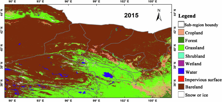
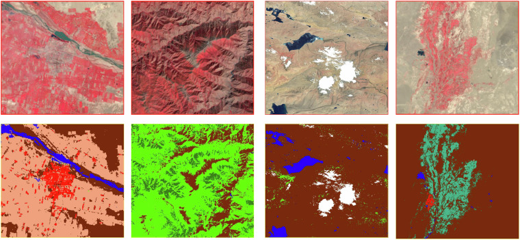
All decision trees for 11 sub-regions are implemented and executed on the GEE platform, significantly improving data retrieval and preprocessing efficiency compared to offline processing. To enhance accuracy and minimize impacts on land cover mapping for other periods, expert visual inspections and corrections are performed. The 2015 land cover map is then generated by integrating the sub-regional land cover maps, as shown in Fig. 6. According to the land cover result, bareland and grassland are the two predominant categories in the QMA, comprising 67.92% and 24.34% of the total area, respectively, followed by cropland (3.94%), water (1.20%), snow or ice (0.89%), forest (0.87%), Impervious surface (0.65%), Shrubland (0.15%), and wetland (0.04%). The classification results exhibit high consistency with Landsat-8/OLI false-color composite images, as showned in Fig. 7.
Fig. 6.
Land cover map of QMA in 2015.
Fig. 7.
Details between land cover map of 2015 (below) compared with landsat-8/OLI false color composite image (above).
Land cover production in other periods
In many existing land cover datasets, the creation of multi-period products is often done independent, which can compromise the accuracy of time series analyses20. To address this, this research followows a two-step process to generate land cover maps for different time periods.
Firstly, the Continuous Change Detection (CCD) algorithm is employed to detect changed pixels by analyzing the monthly composite time series between the target year and a reference year. The CCD algorithm is a time-series-based change detection algorithm specifically designed for remote sensing applications. Originally developed for time series multi-band Landsat images analysis, it models temporal spectral features such as seasonality, trends, and spectral variability. This algorithm’s functions are integrated into the GEE platform, providing direct access and utilization. For mapping land cover in 2010 and 2020, the reference year is 2015; for 2005, the reference year is 2010, an so forth. Secondly, the decision tree method is used to classify these changed pixels into distinct categories. The classification decision tree and rules for changed pixels are consistent with those outlined in Fig. 5 and Table 4.
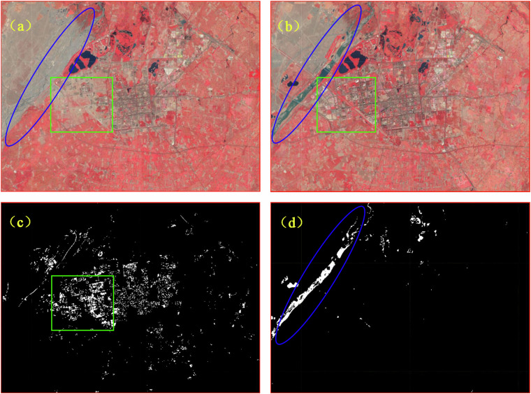
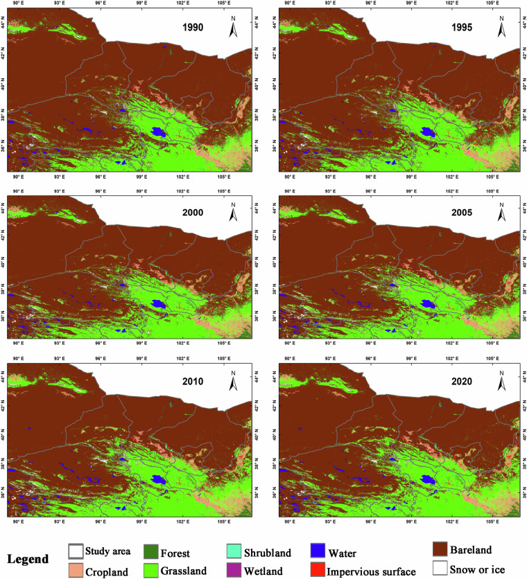
This procedure ensures continuity and comparability between land cover maps from different periods. Figures 8–11 provide detailed insights into the change detection results. Additionally, visual discrimination and correction by specialists are performed as a final refinement step. Figure 12 displays the land cover maps of the study area at various periods, revealing significant spatio-temporal dynamic changes in specific areas.
Fig. 9.
An example of detected new vegetation land. (a) False color composite image of 2015. (b) False color composite image of 2010. (c) New vegetation land highlighted in the green rectangle.
Fig. 10.
An example of detected new cropland. (a) False color composite image of 1990. (b) False color composite image of 1995. (c) New cropland highlighted in the green rectangle.
Fig. 8.
An example of detected new water and impervious surface from 2015 to 2020. (a) False color composite image of 2015. (b) False color composite image of 2020. (c) New impervious surface highlighted in the green rectangle. (d) New water highlighted in the blue oval box.
Fig. 11.
An example of detected new bareland. (a) False color composite image of 2005. (b) False color composite image of 2000. (c) New bareland highlighted in the green rectangle.
Fig. 12.
Land cover maps of QMA in 1990, 1995, 2000, 2005, 2010, 2020.
Data Records
The dataset (QMA_LC30) is avaiable for free access at the National Tibetan Plateau Data Center via 10.11888/Terre.tpdc.30118121. The archive includes files with 7 land cover maps spanning from 1990 to 2020, provided in geographic Lat/Lon projection and Cloud-Optimised GeoTIFF (COG) format. It also contains a classification system document named “ClassificationSystem.docx” and metadata in DOCX format. Each land cover map is named “YYYY_QiLianShan_WholeBasin_LC30.tif”, where “YYYY” represents the respective year.
Technical Validation
Accuracy assessment of multi-period land cover maps separately
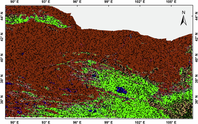
Validation points are selected from Landsat and Google high-resolution images available on the GEE platform by 11 experts with extensive experience in long-term land cover classification. The number of validation points for each category are determined using the hierarchical classification method based on area ratio, with the exception of bareland and grassland due to their disproportionately high coverage (over 92% of the total study area). Both bareland and grassland exhibit high classification accuracy for their distinctive characteristics. Adhering strictly to the hierarchical classification method would result in almost all validation points being classified as bareland or grassland, leading to an overestimation of the overall accuracy. The number of validation points for bareland and grassland are set at 7000 and 4000, respectively, based on feasibility and proportional validation needs. The spatial distribution of validation points is illustrated in Fig. 13.
Fig. 13.
Samples distribution for validation in 2015.
To provide a robust foundation for users relying on maps for specific periods, validation is conducted for each land cover map corresponding to these periods. Metrics such as user’s accuracy, producer’s accuracy, and overall accuracy are calculated. The confusion matrix for the 2015 land cover map is presented in Table 5, while Table 6 displays the validated overall accuracy for all 7 land cover maps. The overall accuracy for all 7 maps exceeds 0.92, indicating high precision of the product. However, shrubland and wetland categories show lower accuracy compared to other categories. The reduced accuracy of wetland may be due to temporal discrepancies between image classification and sample selection, given their high temporal variability. Shrubland presents challenges due to its similarity to sparse forests or certain grasslands, resulting in a complex distribution that is difficult to distinguish at a 30 m resolution. It is also noteworthy that shrubland and wetland show lower user’s accuracy in other global land cover products, with values of 0.73 and 0.75 in GlobeLand30 20105, 0.72 and 0.43 in GLC_FCS30 20158, and 0.63 and 0.34 in FROM_GLC10 20176,7, respectively. Improving the accuracy of shrubland and wetland classification remains a critical area in further research22.
Table 5.
Confusion matrix of the classification in 2015.
| Reference | Wi | User’s | |||||||||||
|---|---|---|---|---|---|---|---|---|---|---|---|---|---|
| Class | Cro. | For. | Gra. | Shr. | Wet. | Wat. | Imp. | Bar. | Sno. | Total | |||
| M A p | Cro. | 1850 | 22 | 73 | 0 | 2 | 0 | 0 | 64 | 0 | 2011 | 3.94 | 0.92 ± 0.01 |
| For. | 22 | 404 | 7 | 3 | 0 | 6 | 1 | 0 | 0 | 443 | 0.87 | 0.91 ± 0.03 | |
| Gra. | 54 | 16 | 3734 | 8 | 1 | 30 | 9 | 146 | 2 | 4000 | 24.34 | 0.94 ± 0.01 | |
| Shr. | 0 | 6 | 11 | 57 | 1 | 3 | 0 | 0 | 0 | 78 | 0.15 | 0.83 ± 0.10 | |
| Wet. | 0 | 0 | 1 | 1 | 16 | 2 | 0 | 0 | 0 | 20 | 0.04 | 0.74 ± 0.18 | |
| Wat. | 1 | 0 | 6 | 7 | 1 | 560 | 0 | 33 | 3 | 611 | 1.20 | 0.92 ± 0.02 | |
| Imp. | 0 | 0 | 2 | 0 | 0 | 10 | 307 | 13 | 0 | 332 | 0.65 | 0.90 ± 0.03 | |
| Bar. | 92 | 0 | 194 | 3 | 0 | 5 | 14 | 6660 | 32 | 7000 | 67.92 | 0.98 ± 0.01 | |
| Sno. | 0 | 3 | 0 | 0 | 1 | 10 | 0 | 10 | 431 | 455 | 0.89 | 0.92 ± 0.02 | |
| Total | 1989 | 451 | 4008 | 79 | 22 | 626 | 381 | 6906 | 488 | 14950 | — | — | |
| Producer’s | 0.74 ± 0.01 | 0.83 ± 0.02 | 0.92 ± 0.01 | 0.53 ± 0.08 | 0.66 ± 0.13 | 0.79 ± 0.02 | 0.76 ± 0.02 | 0.98 ± 0.01 | 0.72 ± 0.02 | — | |||
| Overall | 0.94 ± 0.01 | ||||||||||||
Note: Cro., For., Gra., Shr., Wet., Wat., Imp., Bar., Sno., Use., Pro., and Overall are the abbreviation of cropland, fores, grassland, shrubland, wetland, water, impervious surface, bareland, snow or ice, user’s accuracy, producer’s accuracy, and overall accuracy, respectively. Wi is the proportion of the area mapped as category i.
Table 6.
The validated results of the 7 land cover maps.
| 1990 | 1995 | 2000 | 2005 | 2010 | 2015 | 2020 | |
|---|---|---|---|---|---|---|---|
| Overall | 0.92 ± 0.02 | 0.92 ± 0.02 | 0.94 ± 0.01 | 0.93 ± 0.01 | 0.94 ± 0.03 | 0.94 ± 0.01 | 0.94 ± 0.01 |
Accuracy assessment compared with other land cover products
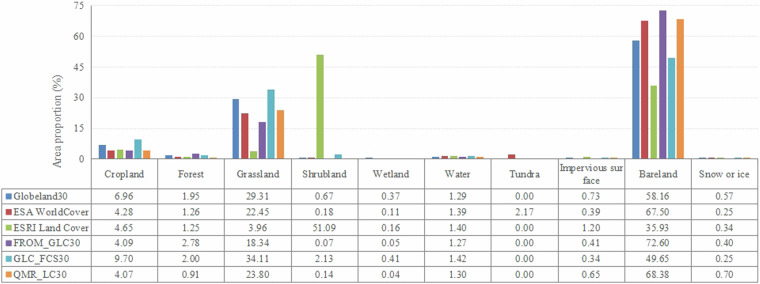
Figures 2, 14 highlight noticeable differences between the QMA_LC30 dataset and others renowned datasets, including GlobeLand30, ESA WorldCover, ESRI 2020 Land Cover, FROM_GLC30, and GLC_FCS30, for the year 2020. Figure 14 illustrates the proportion of area covered by each category in these 6 land cover maps. The performance of each product by category is as follows.
Cropland. GLC_FCS30 identifies the largest cropland area (9.70%), followed by GlobeLand30 (6.96%). QMA_LC30 shows the smallest cropland extent (4.07%), with minimal differences from ESA worldcover (4.28%), ESRI 2020 Land Cover (4.65%), and FROM_GLC30 (4.09%).
Forest. FROM_GLC30 has the most extensive forest coverage (2.78%), while QMA_LC30 identifies the least (0.91%). GlobeLand30 aligns closely with GLC_FCS0 (1.95% and 2.00%), and ESA worldcover closely resembles ESRI 2020 Land Cover (1.26% and 1.25%).
Grassland. GLC_FCS30 dominates this category with the largest proportion (34.11%), followed by GlobeLand30 (29.31%). ESRI 2020 Land Cover has the smallest grassland area (3.96%), while QMA_LC30 aligns more closely with ESA worldcover and FROM_GLC30 (23.80%, 22.45% and 18.34%, respectively).
Shrubland. ESRI 2020 Land Cover stands out with the largest shrubland allocation (51.09%), significantly surpassing other products, while FROM_GLC30 identifies the least (only 0.07%). QMA_LC30 closely resembles ESA worldcover (0.14% and 0.18%).
Wetland. GLC_FCS30 and GlobeLand30 allocate larger proportion (0.41% and 0.37%) compared to other datasets, with QMA_LC30 closely aligning with FROM_GLC30 (0.04% and 0.05%).
Water. The identification of water bodies by different products shows no significantly deviations.
Tundra. Except for ESA WorldCover, other products do not identify tundra, and QMA_LC30 also has no tundra classification.
Impervious surface. ESRI 2020 Land Cover identifies the largest impervious surface (1.20%), followed by GlobeLand30 (0.73%) and QMA_LC30 (0.65%). ESA worldcover, FROM_GLC30 and GLC_FCS30 show comparable proportions (0.39%, 0.41% and 0.34%, respectively).
Bareland. FROM_GLC30 records the highest bareland proportion (72.60%), with QMA_LC30 and GlobeLand30 following closely (68.38% and 67.50%), while ESRI 2020 Land Cover indicates the smallest bareland coverage (35.93%).
Snow or ice. QMA_LC30 and GlobeLand30 display larger extents (0.70% and 0.57%) compared to other datasets, with ESA worldcover and GLC_FCS30 showing the smallest percentages (both 0.25%).
Fig. 14.
Comparison of the area percentages for 6 land cover maps in QMA at 2020.
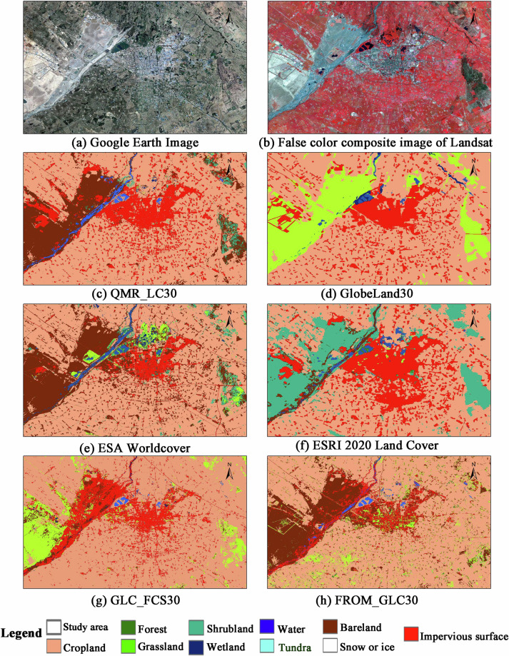
Figure 15 provides a detailed comparison near ZhangYe city, GanSu province, in 2020. It is evident that the QMA_LC30 demonstrates the highest alignment with both the Google Earth and Landsat image. GlobeLand30 shows a substantial amount of grassland, while ESRI 2020 Land Cover emphasizes more shrubland. ESA WorldCover closely resembles QMA_LC30. ESRI 2020 Land Cover delineates a greater impervious surface, contrasting with FROM_GLC30, which shows less. Both FROM_GLC30 and GLC_FCS30 struggle with accuracy in distinguishing between bareland and impervious surfaces. Notably, ESA WorldCover excels in identifying roads, surpassing even QMA_LC30 in this regard. On the other hand, GlobeLand30, ESRI 2020 Land Cover, GLC_FCS30, and FROM_GLC30 show lower accuracy in distinguishing water bodies and wetlands. GlobeLand30 frequently misclassifies numerous water bodies and wetlands as grassland, whereas ESRI 2020 Land Cover often assigns them to the bareland category.
Fig. 15.
Comparison of several Land cover maps in 2020. (a) Google Earth image. (b) False color composite image of Landsat. (c) QMA_LC30. (d) GlobeLand30. (e) ESA Worldcover. (f) ESRI 2020 Land Cover. (g) GLC_FCS30. (h) FROM_GLC30.
Among these 6 land cover maps analyzed, only 36.65% of pixels share an identical classification code. Table 7 details the numbers and proportions of pixels with matching codes for each land cover category in comparison to QMA_LC30. Notably, ESA WorldCover shows the highest consistency with QMA_LC30 at 86.91%, followed closely by FROM_GLC30 at 86.66%. In contrast, ESRI 2020 Land Cover exhibits the most significant deviation from QMA_LC30, with only 43.92% of pixels matching.
Table 7.
The numbers and proportions of pixels with same category for each land cover categary of other products compared with QMA_LC30 (the highlighted in bold value indicates the highest consistency with QMA_LC30 than others).
| Class | GlobeLand30 | ESA Worldcover | ESRI 2020 Land Cover | FROM_GLC30 | GLC_FCS30 |
|---|---|---|---|---|---|
| Cro. | 5.26E + 07 | 4.17E + 07 | 3.98E + 07 | 3.95E + 07 | 5.11E + 07 |
| For. | 1.08E + 07 | 1.15E + 07 | 1.08E + 07 | 1.28E + 07 | 1.25E + 07 |
| Gra. | 2.98E + 08 | 3.11E + 08 | 6.71E + 07 | 2.68E + 08 | 3.16E + 08 |
| Shr. | 8.38E + 04 | 9.46E + 05 | 2.11E + 06 | 8.59E + 04 | 1.32E + 05 |
| Wet. | 2.71E + 05 | 3.17E + 05 | 4.35E + 05 | 3.93E + 04 | 2.29E + 04 |
| Wat. | 1.92E + 07 | 2.05E + 07 | 2.02E + 07 | 1.97E + 07 | 2.01E + 07 |
| Imp. | 6.23E + 06 | 4.03E + 06 | 9.87E + 06 | 2.85E + 06 | 4.38E + 06 |
| Bar. | 9.68E + 08 | 1.11E + 09 | 6.05E + 08 | 1.15E + 09 | 8.35E + 08 |
| Sno. | 5.61E + 06 | 4.04E + 06 | 4.97E + 06 | 5.23E + 06 | 4.94E + 06 |
| Total | 5.26E + 07 | 4.17E + 07 | 3.98E + 07 | 3.95E + 07 | 5.11E + 07 |
| Proportion(%) | 78.68 | 86.91 | 43.92 | 86.66 | 79.65 |
Table 7 hightlights in blue the values that demonstrate greater consistency with QMA_LC30 compared to other datasets within each category. It is evident that GlobeLand30 aligns most closely with QMA_LC30 in cropland and snow or ice, while ESA WorldCover excels in water classification. ESRI 2020 Land Cover shows superior performance in delineating shrubland, wetland, and impervious surfaces, while FROM_GLC30 displays the highest consistency in forest and bareland categories. Additionally, GLC_FCS30 is the closest match to QMA_LC30 in grassland.
To further assess accuracy, pixels with conflicting classification codes between QMA_LC30 and ESA WorldCover are selected as the validation set. The results indicate that 54.03% of these pixels are accurately classified in QMA_LC30, compared to only 22% in ESA WorldCover. This outcome underscores QMA_LC30’s higher accuracy in handling pixels with inconsistent classification codes compared to ESA WorldCover.
Overall, while products like GlobeLand30 boast global accuracy exceeding 80%, they still exhibit notable deficiencies at regional scales, particularly in complex terrains such as the QMA. In contrast, QMA_LC30 offers better suitability and enhanced accuracy for this area. However, it is important to acknowledge that the validation results presented in this study also have some uncertainties.
Firstly, discrepancies arise from variations in classification systems. The original GLC_FCS30 dataset comprises 29 categories, including distinctions like rainfed cropland, herbaceous cover, and evergreen broadleaved forest. For comparison purpose, this study condensed these 29 categories into 10 based on their definitions. However, this merging process may have inadvertently combined ambiguous categories. For example, the classification “sparse vegetation” in GLC_FCS30, defined as “fc < 0.15,” lacks clarity regarding whether it denotes grassland, shrubland, or sparse trees. In this study, it is assimilated into the grassland category, potentially introducing uncertainty.
Secondly, discrepancies in the remote sensing images used by these products can also contribute to uncertainties in the classification outcomes. Temporal variations in the images, resulting from factors like seasonal changes, can influence the identification of features such as water bodies or wetlands. During dry seasons, certain water bodies may desiccate, resembling riverbanks or bareland in remote sensing images. Conversely, in the rainy season, dense aquatic vegetation may cause these areas to resemble grasslands. Such temporal disparities can lead to inconsistencies in classification results.
Analysis of times series changes
The changes in catagories from 1990 to 2020 have also been validated to demonstrate the advantages of this product in dynamis change monitoring. The validation process categorized pixels into two groups: changed and unchanged. Validation points are selected based on Landsat images. Table 8 lists the number of validation points and confusion matrix. The user’s and producer’s accuracy of the changed pixels both reached 0.90, while for the unchanged pixels, both reached 0.92. The overall accuracy is 0.91, indicating that the QMA_LC30 effectively reflecst the changes that occurred between 1990 and 2020.
Table 8.
The confusion matrix of changed and unchanged pixels between 1990 and 2020.
| Reference | User’s | Producer’s | Overall | ||||
|---|---|---|---|---|---|---|---|
| Class | Changed | Unchanged | Total | ||||
| Map | Changes | 2296 | 268 | 2564 | 0.90 | 0.90 | 0.91 |
| Unchanged | 264 | 3034 | 3298 | 0.92 | 0.92 | ||
| Total | 2560 | 3302 | 5862 | — | — | ||
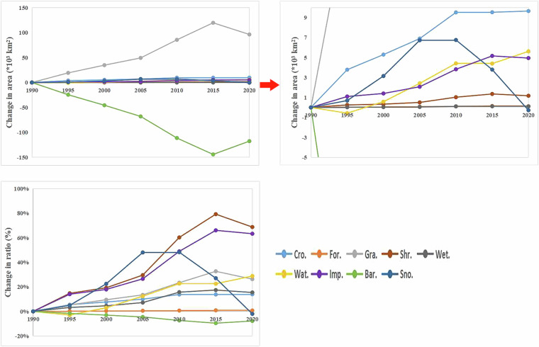
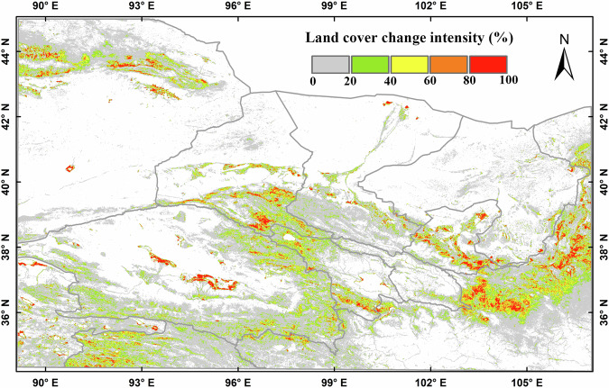
Figure 16 shows the net change in area and the ratio of land cover types from 1990 to 2020, while Fig. 17 displays the intensity of land cover changes over the same period by calculating the proportions of changed pixels within a 0.01-degree grid. It is evident that each land cover category has experienced varying degrees of change.
Grassland has seen the most significant increases, while bareland has experienced the greatest decreases. This is because, in arid and semi-arid regions, grassland and bareland are highly sensitive to climate change. During years with higher temperatures and incresed rainfall, bareland often converts to grassland, whereas during drier periods, grassland can revert to bareland. A previous study by Duan et al. (2022) demonstrated that precipitation in the QMA has generally increased from 1990 to 2020, which aligns with the observed changes in grassland and bareland.
Areas with higher intensity of change are primarily concentrated in cropland and impervious surfaces near human settlements, highlighting the sigificant impact of human activities on land cover. The growth of cropland was particularly pronounced before 2010, with an increase of 9,520 km2, representing a 15.68% rise. This expansion was driven by the need to meet the growing food demands of a rapidly increasing population, leading to extensive cultivation of new cropland. However, after 2010, due to government policies focused on ecological protection, such as returning farmland to forests, along with the reduced demand for cropland by the growth of other industries, the cropland area has slightly decreased and has since stabilized.
The forest area did not undergo significant changes before 2010 but showed a slight upward trend afterward The increase is likely due to the policy of returning farmland to forests as well as an increase in rainfall.
The area of water bodies declined between 1990 and 1995 but gradually increased after 1995. This trend is closely related to climate change and national policies. On one hand, rising temperatures and increasing precipitation have contributed to the expansion of water bodies. On the other hand, since 2000, the goverment has implemented a series of ecological and environmental protection policies aimed at address issues like land degradation and sandstorms, which have enhanced the water storage capacity of major rivers.
The overall trend of impervious surfaces is increasing, with a rapid growth rate observed between 2000 and 2015, followed by a slower rate between 2015 and 2020. This pattern reflects the extensive infrastructure and construction projects that took place from 2000 to 2015, including housing developments, expansion projects, and construction of hydropower station, during a period of rapid development in the QMA and across China. After 2015, as infrastructure improvements researched a more advanced stage and ecological and environment protection gained greater emphasis, the rate of increase in impervious surfaces slowed down.
Snow and ice cover showed an upward trend in 2005 but sharply decreased after 2010. However, it is important to note that this dataset is not sufficient to support a comprehensive study of glacier changes. The temporal limitations of remote sensing data mean that the glacier snow cover captured in this dataset reflects the conditions at the time of image acquisition rather than the true extent of permanent glacier snow cover. This represents a limitation of this dataset.
Fig. 16.
The net changed area and ratio of land cover types from 1990 to 2020.
Fig. 17.
The land cover change intensity from 1990 to 2020 at 0.01 degrees’ resolution.
Usage Notes
The dataset has been published and is available for free download. When using it, please keep the following points in mind:
The land cover map for the target year may have been generated using images from two years before and after, which could result in some inconsistencies with the actural land cover of the target year. For example, the land cover map for 2010 is produced using images from 2009, 2010, and 2011.
The snow or ice category in these land cover maps does not represent permanent glacier and snow cover but rather reflects the conditions at the time of remote sensing image capture.
Acknowledgements
This study is supported by the National Key Research and Development Program of China (No.2021YFE0194700), and the Science and Technology Fundamental Resources Investigation Program of China (No. 2022FY100200). The authors thank the National Tibetan Plateau Data Center (https://www.tpdc.ac.cn/home) for providing a platform to share, download, and utilize the datasets.
Author contributions
A.Y. conceived this research, produced all the land cover maps, and wrote the manuscript. B.Z. contributed to the conception and provided guidance. X.W. and A.F. offered guidance, edits and suggestions. L.H., K.A., Q.Z., S.W., B.D. and J.W. validated the dataset.
Code availability
The methodologies used in this study are not fully automated and involve manual intervention, including visual discrimination and interpretation of various land cover maps. Therefore, no code is provided with this dataset.
Competing interests
The authors declare no competing interests.
Footnotes
Publisher’s note Springer Nature remains neutral with regard to jurisdictional claims in published maps and institutional affiliations.
References
- 1.Liu, L., Zhang, X., Gao, Y., Chen, X. & Mi, J. Finer-resolution mapping of global land cover: recent developments, consistency analysis, and prospects. J. Remote Sens.1, 38 (2021). [Google Scholar]
- 2.Zhong, B. et al. Finer resolution land-cover mapping using multiple classifiers and multisource remotely sensed data in the heihe river basin. IEEE J-STARS.8(10), 4973–4992 (2016). [Google Scholar]
- 3.Friedl, M. A. et al. Global land cover mapping from modis: algorithms and early results. Remote Sens. Environ.83(1-2), 287–302 (2002). [Google Scholar]
- 4.Zhong, B. et al. Land cover mapping using time series HJ-1/CCD data. Sci. China Earth Sci.57, 1790–1799 (2014). [Google Scholar]
- 5.Chen, J. et al. Global land cover mapping at 30 m resolution: A POK-based operational approach. ISPRS J Photogramm103, 7–27 (2015). [Google Scholar]
- 6.Gong, P., Wang, J., Yu, L., Zhao, Y. & Chen, J. Finer resolution observation and monitoring of global land cover: first mapping results with Landsat tm and ETM+ data. Int. J Remote Sens.34(7), 48 (2013). [Google Scholar]
- 7.Gong, P. et al. Stable classification with limited sample: Transferring a 30-m resolution sample set collected in 2015 to mapping 10-m resolution global land cover in 2017. Sci. Bull64, 370–373 (2019). [DOI] [PubMed] [Google Scholar]
- 8.Zhang, X. et al. GLC_FCS30: Global land-cover product with fine classification system at 30 m using time-series Landsat imagery. Earth Syst Sci Data13(6), 2753–2776 (2020). [Google Scholar]
- 9.Zanaga, D. et al. ESA WorldCover 10 m 2020 v100.10.5281/zenodo.5571936 (2021). [Google Scholar]
- 10.Karra, K. et al. Global land use/land cover with Sentinel 2 and deep learning. In 2021 IEEE IGARSS (pp. 4704–4707) (July, 2021).
- 11.Tu, Y., Lang, W., Yu, L., Li, Y. & Xu, B. Improved mapping results of 10 m resolution land cover classification in guangdong, china using multisource remote sensing data with google earth engine. IEEE J-STARS13, 5384–5397 (2020). [Google Scholar]
- 12.Gorelick, N. et al. Google Earth Engine: Planetary-scale geospatial analysis for everyone. Remote Sens. Environ.202, 18–27 (2017). [Google Scholar]
- 13.Tamiminia, H. et al. Google Earth Engine for geo-big data applications: A meta-analysis and systematic review. ISPRS J Photogramm164, 152–170 (2020). [Google Scholar]
- 14.Chen, B., Jin, Y. & Brown, P. Automatic mapping of planting year for tree crops with Landsat satellite time series stacks. ISPRS J Photogramm151, 176–188 (2019). [Google Scholar]
- 15.Silva Junior, C. A. D. et al. Mapping soybean planting area in midwest Brazil with remotely sensed images and phenology-based algorithm using the Google Earth Engine platform. Comput. Electron. Agr169, 105194 (2020). [Google Scholar]
- 16.Oliphant, A. J. et al. Mapping cropland extent of Southeast and Northeast Asia using multi-year time-series Landsat 30-m data using a random forest classifier on the Google Earth Engine Cloud. Int. J Appl. Earth Obs.81, 110–124 (2019). [Google Scholar]
- 17.Brovelli, M. A., Sun, Y. & Yordanov, V. Monitoring forest change in the amazon using multi-temporal remote sensing data and machine learning classification on Google Earth Engine. ISPRS Int. J Geo-Inf.9(10), 580 (2020). [Google Scholar]
- 18.Yang, X. et al. Monthly estimation of the surface water extent in France at a 10-m resolution using Sentinel-2 data. Remote Sens. Environ.244, 111803 (2020). [Google Scholar]
- 19.Huang, H. et al. Mapping major land cover dynamics in Beijing using all Landsat images in Google Earth Engine. Remote Sens. Environ.202, 166–176 (2017). [Google Scholar]
- 20.Sulla-Menashe, D., Gray, J. M., Abercrombie, S. P. & Friedl, M. A. Hierarchical mapping of annual global land cover 2001 to present: the modis collection 6 land cover product. Remote Sens. Environ222, 183–194 (2019). [Google Scholar]
- 21.Yang, A. & Zhong, B. 30m 5-yearly land cover maps of Qilian Mountain Area from 1990 to 2020. National Tibetan Plateau/Third Pole Environment Data Center.10.11888/Terre.tpdc.301181 (2024). [DOI] [PMC free article] [PubMed] [Google Scholar]
- 22.Zhong, B., Yang, L., Luo, X., Wu, J. & Hu, L. Extracting Shrubland in Deserts from Medium-Resolution Remote-Sensing Data at Large Scale. Remote Sens16, 374 (2024). [Google Scholar]
- 23.Ran, Y. & Li, X. MICLCover land cover map of the Heihe river basin (2000). National Tibetan Plateau Data Center10.3972/westdc.010.2013.db.heihe (2013). [Google Scholar]
- 24.Ran, Y. H., Li, X., Lu, L. & Li, Z. Y. Large-scale land cover mapping with the integration of multi-source information based on the Dempster-Shafer theory. Int J Geogr Inf SCI26(1), 169–191 (2012). [Google Scholar]
- 25.Liu, J. & Wang, J. Landuse/landcover dataset of the Heihe river basin (1980s). National Tibetan Plateau Data Center10.3972/heihe.021.2013.db (2013). [Google Scholar]
- 26.Wang, J. & Liu, J. Landuse/Landcover data of the Heihe river basin (2000). National Tibetan Plateau Data Center10.3972/heihe.020.2013.db (2013). [Google Scholar]
- 27.Wang, J. Landuse/landcover data of the Heihe River Basin in 2000. National Tibetan Plateau Data Center10.3972/heihe.039.2014.db (2015). [Google Scholar]
- 28.Hu, X., Lu, L., Li, X., Wang, J. & Guo, M. Land use/cover change in the middle reaches of the Heihe river basin over 2000–2011 and its implications for sustainable water resource management. PloS one10(6), e0128960 (2015). [DOI] [PMC free article] [PubMed] [Google Scholar]
- 29.Zhong, B. & Yang, A. HiWATER: Land cover map of the Heihe River Basin. National Tibetan Plateau Data Center10.3972/hiwater.155.2014.db (2016). [Google Scholar]
- 30.Qi, Y., Zhang, J., Yan, C., Duan, H. & Jia, Y. The land cover/use data in key areas of the Qilian Mountain (2018). National Tibetan Plateau Data Center10.11888/Geogra.tpdc.270154 (2019). [Google Scholar]
- 31.Yan, C. Land use/land cover dataset of Zhangye city in 2005. National Tibetan Plateau Data Center10.3972/heihe.011.2013.db (2013). [Google Scholar]
- 32.Hu, X., Wang, J. & Li, X. Landuse/landcover data of Zhangye city (2007). National Tibetan Plateau Data Center10.3972/heihe.018.2013.db (2015). [Google Scholar]
- 33.Hu, X., Lu, L., Li, X., Wang, J. & Lu, X. Ejin oasis land use and vegetation change between 2000 and 2011: The role of the Ecological Water Diversion Project. Energies8(7), 7040–7057 (2015). [Google Scholar]
- 34.Liu, J., Zhuang, D., Wang, J., Zhou, W., Wu, S. Landcover dataset of the Shulehe River Basin (2000). National Tibetan Plateau Data Center. (2014).
- 35.Liu, J., Zhuang, D., Wang, J., Zhou, W., Wu, S. Landuse/Landcover data of the QinghaiLake River Basin (2000). National Tibetan Plateau Data Center. (2014).
Associated Data
This section collects any data citations, data availability statements, or supplementary materials included in this article.
Data Availability Statement
The methodologies used in this study are not fully automated and involve manual intervention, including visual discrimination and interpretation of various land cover maps. Therefore, no code is provided with this dataset.


