Fast computational E-field dosimetry for transcranial magnetic stimulation using adaptive cross approximation and auxiliary dipole method (ACA-ADM)

Abstract

Transcranial Magnetic Stimulation (TMS) is a non-invasive brain stimulation technique that uses a coil to induce an electric field (E-field) in the brain and modulate its activity. Many applications of TMS call for the repeated execution of E-field solvers to determine the E-field induced in the brain for different coil placements. However, the usage of solvers for these applications remains impractical because each coil placement requires the solution of a large linear system of equations. We develop a fast E-field solver that enables the rapid evaluation of the E-field distribution for a brain region of interest (ROI) for a large number of coil placements, which is achieved in two stages. First, during the pre-processing stage, the mapping between coil placement and brain ROI E-field distribution is approximated from E-field results for a few coil placements. Specifically, we discretize the mapping into a matrix with each column having the ROI E-field samples for a fixed coil placement. This matrix is approximated from a few of its rows and columns using adaptive cross approximation (ACA). The accuracy, efficiency, and applicability of the new ACA approach are determined by comparing its E-field predictions with analytical and standard solvers in spherical and MRI-derived head models. During the second stage, the E-field distribution in the brain ROI from a specific coil placement is determined by the obtained rows and columns in milliseconds. For many applications, only the E-field distribution for a comparatively small ROI is required. For example, the solver can complete the pre-processing stage in approximately 4 hours and determine the ROI E-field in approximately 40 ms for a 100 mm diameter ROI with less than 2% error enabling its use for neuro-navigation and other applications. Highlight: We developed a fast solver for TMS computational E-field dosimetry, which can determine the ROI E-field in approximately 40 ms for a 100 mm diameter ROI with less than 2% error.

1. Introduction

Transcranial Magnetic Stimulation (TMS) is a non-invasive method for brain stimulation that uses a coil driven by low-frequency current pulses (≤ 10kHz) to magnetically stimulate targeted brain regions. TMS has been widely used for neuroscience research to study brain function and for the treatment of depression, migraines, and others (Carmi et al., 2019; Cohen et al., 2022; Couturier, 2005; De Ridder et al., 2007; Hoffman et al., 2005; Kaptsan et al., 2003; Lan et al., 2017; Lipton et al., 2010; Nahas et al., 2003; O’Reardon et al., 2007; Pascual-Leone et al., 1996). It is recognized that neurons in brain regions exposed to an electric field (E-field) above a stimulation threshold are likely stimulated during TMS (Aberra et al., 2020; Siebner et al., 2022). Correspondingly, E-field dosimetry can be used to infer its effects. For example, in cortical motor mapping, body movements are measured from motor evoked potentials (MEPs) via electrodes. These MEPs are then correlated with an E-field related quantity to predict its cortical representation (Weise et al., 2020). Moreover, E-field predictions can be used to determine TMS coil placements that both maximizes on-target and minimizes off-target E-field exposure (Balderston et al., 2020; Casarotto et al., 2022; Dannhauer et al., 2022; Lynch et al., 2022). The E-field distribution is also critical for coil shape optimization (Gomez et al., 2018; Gomez-Tames et al., 2018; Koponen et al., 2017) and determining TMS coil driving current and other parameters (Beynel et al., 2020). All these applications benefit from a simulation method that given a coil and head model can determine the E-field distribution rapidly and accurately. Currently, different approaches have been proposed to directly determine the E-field in the ROI of an MRI-derived head model, such as the finite difference method (FDM) (Laakso and Hirata, 2012; Toschi et al., 2008), finite element method (FEM) (Dannhauer et al., 2012; Goetz and Deng, 2017), or boundary element method (BEM) (Gomez et al., 2020; Makarov et al., 2019; 2018; Stenroos and Koponen, 2019). TMS cortical mapping, coil placement, and uncertainty analysis could be improved by using the E-field distribution in the brain for many coil positions and orientations. However, the time required to run these solvers makes them ill-suited for repeated execution. For example, to evaluate the TMS-induced E-field for a single coil placement using SimNIBS FEM (Saturnino et al., 2019), or BEM accelerated with the fast multipole method (FMM) (Makarov et al., 2020) takes tens of seconds to minutes.

To evaluate the E-field efficiently for TMS, we recently proposed the auxiliary dipole method (ADM)(Gomez et al., 2021), which applies reciprocity to compute the average E-field in a brain ROI. ADM can compute the average E-field in an ROI generated by over one million coil placements in under 5 minutes. However, this method only provides the average ROI E-field and does not compute its distribution. Other common statistical metrics used to analyze TMS induced E-fields that are less prone to outliers such as median, percentiles or E100 cannot be determined using ADM (Beynel et al., 2020; Dannhauer et al., 2022). Furthermore, in some applications the E-field must be maximized in the ROI while minimized elsewhere. Since ADM only computes average E-fields this cannot be done using ADM. As a result, ADM can result in coil placements where functional networks other than the target receive equivalent or greater levels of stimulation than the target network (Lynch et al., 2022). There have been attempts to create real-time and near real-time E-field solvers that determine the E-field distribution in fractions of a second and a few seconds, respectively. All these methods have limitations as detailed the next paragraph. For many applications, only the E-field distribution for a comparatively small ROI is required. Furthermore, ROI E-field distributions for a dense sampling of coil placements can be used to determine optimum coil placement, or can be interpolated for determining the E-field rapidly on-the-fly. Unlike the real-time solvers, our method develops a dense sampling of the coil placement to E-field distribution map.

By focusing on fixed coil placements our method can achieve more computationally efficient results than the (or near) real-time E-field solvers recently proposed. A deep-learning-based E-field solver was proposed for real-time E-field analysis (Yokota et al., 2019). While this approach delivers visually accurate E-fields, the errors are not as low as standard E-field solvers (or the ones achieved by our method). A highly optimized BEM solver was developed for real-time E-field estimation (Stenroos and Koponen, 2019). However, unlike our solver, their approach requires computation time scaling with mesh resolution, limiting its use for meshes that have lower resolution than those used for standard FEM (Stenroos and Koponen, 2019). More recently, the magnetic stimulation profile approach was applied for real-time E-field evaluation, which, after a setup time of up to 10.6 hours, can determine the E-field in 0.1 seconds (Daneshzand et al., 2021) on triangle meshes consisting of up to 250 thousand triangles. While the magnetic stimulation profile approach is a highly efficient method, the accurate determination of the E-field using magnetic dipoles still requires over 1500 magnetic dipoles to achieve an relative error between 5–15%. Here we adopt a matrix approximation approach and are able predict the whole head E-field using less than or equal to 192 modes and achieve a relative error less than 2% in the whole head.

Our method uses FEM and ADM simulations to develop an interpolant for the coil placement to cortical E-field mapping. This interpolant is generated by using a matrix to approximate the mapping between coil placement and cortical E-fields. The interpolant is then generated using the adaptive cross approximation (ACA) to compress the matrix. The ACA method was first proposed to compress the low-rank off-diagonal blocks of matrices resulting from the approximation of integral equations with non-oscillatory kernels (Bebendorf, 2011; Bebendorf and Rjasanow, 2003; Zhao et al., 2005). For TMS, the sources reside outside the head and the goal is to determine the E-field in the brain. This matrix will have the same spectral properties as a source to target (S2T) operator corresponding to the composition of the source to multipole (S2M), multipole to local (M2L), and local to target (L2T) operators in a kernel-independent FMM for non-oscillatory kernels (Ying et al., 2004). These operators, and by proxy their composition, are known to be low-rank. As a result, the coil position to E-field matrix will be compressible by ACA. In fact, the ACA enables us to generate an approximation to the E-field distribution on a 20 mm region with less than 2% relative error by running a FEM solver and ADM for less than 20 coil placements and ROI tetrahedra, respectively. This results in a total 78 minutes long pre-processing time and 0.1 ms to access the ROI E-field distribution for a large number of coil positions on a computer with 2.90 GHz Intel(R) Core(TM) i7–10700 CPU.

This paper is organized as follows: The method section describes the details of the proposed ACA-ADM approach, head models, ROIs, and some benchmark metrics used in this study. The results section provides results that benchmark the ACA-ADM by comparing it with the E-field obtained from ADM and analytical approaches. Furthermore, we consider results obtained using the ACA-ADM for several coil placement tasks including a motor mapping study and maximizing on-target stimulation while minimizing off-target stimulation. Our results indicate that the ACA-ADM can achieve less than 2% error for several ROI sizes requiring a minimal number of FEM solver runs and that the ACA-ADM is a practical tool that can be used for optimizing TMS coils placement for a variety of TMS targeting objectives.

2. Methods

2.1. Overview

We consider coil placements flat on the scalp centered about N_c distinct coil positions (Fig. 1). For each coil position, we consider 360 orientations, each generated by rotating the coil 1° about the normal of the scalp at the coil center. The ROI is composed of N_t gray matter (GM) and white matter (WM) tetrahedra located in a spherical region centered about a location r_ROI and with diameter d_ROI. The ROI E-field is stored in a two-dimension table with entries defined as

$${\mathit{Z}}_{3\left(i_1-1\right)+i_2,360\left(j_1-1\right)+j_2}=\left\{\begin{array}{ll}{\mathit{E}}_{j_1}^{\left(j_2\right)}\left({\mathit{r}}_{i_1}\right)\cdot \widehat{x}\hfill & i_2=1\hfill \\ {\mathit{E}}_{j_1}^{\left(j_2\right)}\left({\mathit{r}}_{i_1}\right)\cdot \widehat{y}\hfill & i_2=2,\hfill \\ {\mathit{E}}_{j_1}^{\left(j_2\right)}\left({\mathit{r}}_{i_1}\right)\cdot \widehat{z}\hfill & i_2=3\hfill \end{array}\right.$$ (1)

where i₁ = 1, 2, ⋯ , N , i₂ = 1, 2, 3, j₁ = 1, 2, ⋯ , N , j₂ = 1, 2, ⋯ , 360 and ${\mathit{E}}_{j_1}^{(j_2)}\left({\mathit{r}}_{i_1}\right)$ is the E-field generated at the center of the $i_1^{\text{th}}$ ROI tetrahedron ${\mathit{r}}_{i_1}$ assuming the coil is placed centered at the $j_1^{\text{th}}$ node and oriented to point j₂ degrees clockwise from the back of the head. Fig. 1 illustrates the correspondence between table entries and simulation results. Each column of the table contains the average E-field in each tetrahedron of the ROI mesh assuming a fixed coil placement. For example, in Fig. 1(a), coil placements C₁, C₂, ⋯, C_N correspond to the E-fields stored in Columns 1, 2, ⋯, N (N = 360N_c), respectively. Furthermore, for each $j_1^{\text{th}}$ coil position, there are 360 coil orientations. Correspondingly, each row of the table contains a Cartesian component of the E-field at the center of a fixed ROI mesh tetrahedron for each coil placement. More importantly, since the coil resides outside of the head, this table will be low-rank when viewed as a matrix (Ilmoniemi and Sarvas, 2019; Koponen et al., 2015). This property has been shown analytically for a spherical head where the eigenvalues of the coupling matrix between sources outside of the head and E-fields inside it are known to decay exponentially (Gomez et al., 2018; Koponen et al., 2015). Furthermore, this is the basis for FMM for non-oscillatory kernels (Rokhlin, 1985; Ying et al., 2004). Therefore, as a pre-processing step, we use the ACA method to compress the whole low-rank matrix by computing just a few of its columns and rows. Then, the ROI E-field distribution for a given coil placement can be determined rapidly by multiplying the compressed data structures to determine the corresponding column of the matrix.

Fig. 1.

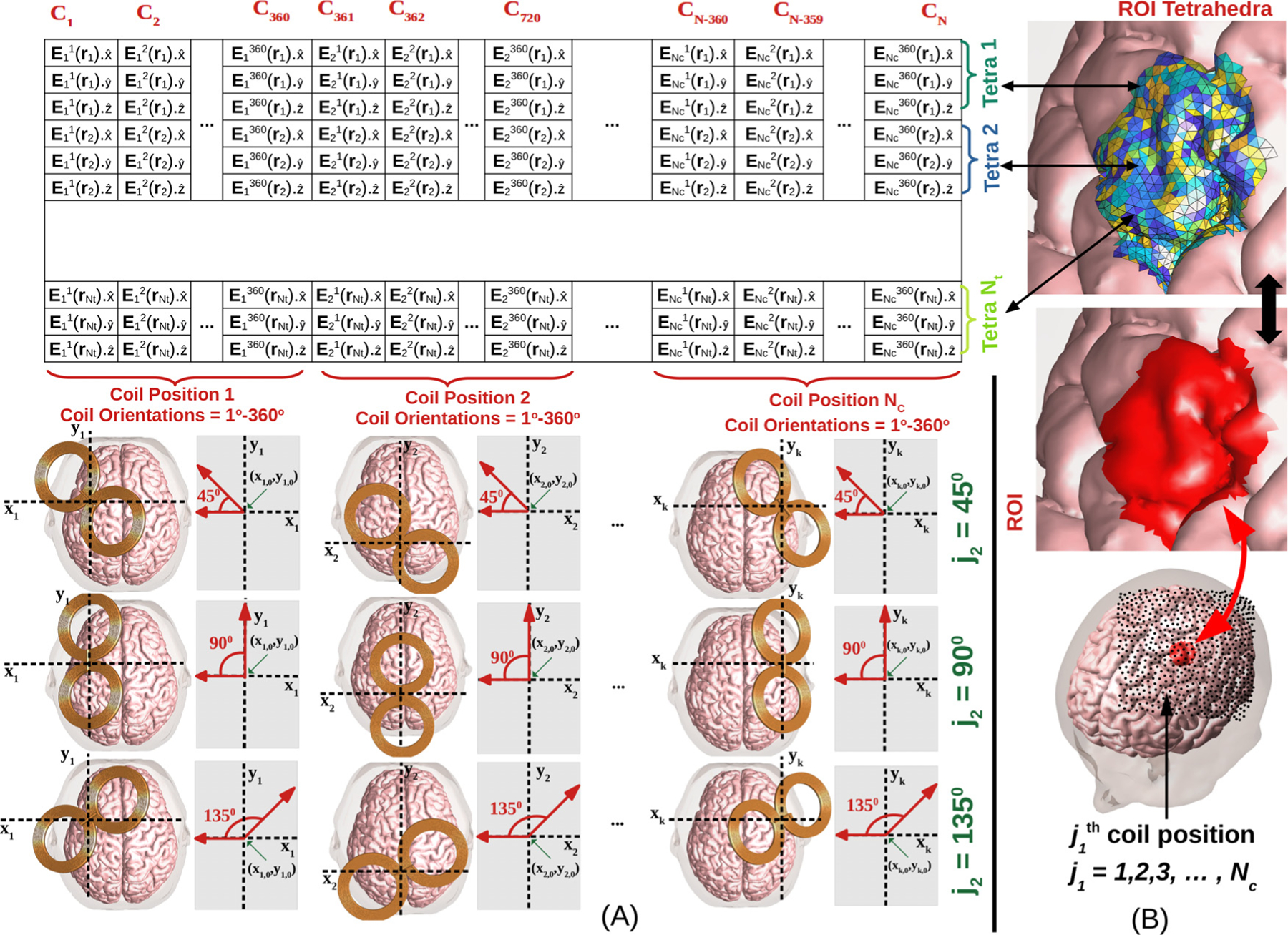
(A) The coil placement to E-field mapping table contains E-fields in the ROI for all coil placements, where N_t is the number of tetrahedra in ROI, N_c is the number of coil positions, and N is the number of coil placements (N = 360N_c). Each column of the table is the induced E-field in every ROI tetrahedron for a fixed coil placement. Each row of the table denotes the E-field induced in a fixed tetrahedron for all possible coil placements. For each coil placement, orientations are defined by rotating the coil tangent to the scalp and about its center as shown. Here a local coordinate axis $\left(x_{j_1},y_{j_1}\right)$ tangential to the scalp and centered about the coil is defined by setting the ${\widehat{y}}_{j_1}$ unit vector pointing posterior to anterior. The angles are defined as the polar angle on this coordinate system. Example coil orientations corresponding to j₂ = 45° , 90° , and 135° are shown for several coil positions. (B) TMS coil positions are denoted by black dots over the scalp of the head model and are typically chosen on a large region covering the ROI (red region).

In the following sections, we will first describe the FEM and ADM used to compute columns and rows of the matrix, respectively. Then, we will describe the ACA algorithm for computing the compressed form of the table shown in Fig. 1. Finally, we will provide details of the coil and head models and benchmark error metrics used in this study.

2.2. Evaluation of a column using the FEM

When the coil is placed at position j₁ and oriented along the $j_2^{\text{th}}$ orientation, it generates an E-field in free-space (i.e. the primary E-²field) denoted as ${\mathit{E}}_{p,j_1}^{(j_2)}\left(\mathit{r}\right)$. Quasi-stationary assumptions dictate that the total E-field is

$${\mathit{E}}_{j_1}^{(j_2)}\left(\mathit{r}\right)=-\nabla \text{Φ}\left(\mathit{r}\right)+{\mathit{E}}_{p,j_1}^{(j_2)}\left(\mathit{r}\right)$$ (2)

and

$$\nabla \cdot \sigma \left(\mathit{r}\right)\nabla \text{Φ}\left(\mathit{r}\right)=\nabla \cdot \sigma \left(\mathit{r}\right){\mathit{E}}_{p,j_1}^{(j_2)}\left(\mathit{r}\right),$$ (3)

where Φ(r) is the scalar potential, σ(r) is the conductivity, and the normal component of ${\mathit{E}}_{j_1}^{(j_2)}\left(\mathit{r}\right)$ is zero on the scalp. To determine ∇Φ(r), we use an in-house 1st order FEM method (for details see Gomez et al. (2020)). The above solution enables us to compute a column of the matrix Z, with the run-time equal to a single FEM solution.

2.3. Evaluation of a row using the ADM

We need to determine a Cartesian component of the E-field at the center of a fixed ROI tetrahedron for all coil placements. This is done using ADM (Gomez et al., 2021). Here, we explain ADM as it pertains to this work. For additional details about ADM, see Gomez et al. (2021). Specifically, we define a constant current inside a tetrahedron equal to ${\mathit{J}}_{i_1}^{(i_2)}\left(\mathit{r}\right)={1/V}_{i_1}\widehat{\mathit{t}}$, where $\widehat{\mathit{t}}$ is $\widehat{\mathit{x}}$, $\widehat{\mathit{y}}$, and $\widehat{\mathit{z}}$ when i₂ is 1, 2, and 3, respectively. i₁ and $V_{i_1}$ are the index of the tetrahedron and its volume, respectively. This current will generate additional conduction currents that are determined using current continuity. Then, the magnetic fields (H-fields) generated outside of the head ${\mathit{H}}_{i_1}^{(i_2)}\left(\mathit{r}\right)$ by the total electric currents inside the head (i.e., the ROI tetrahedron and conduction currents) are determined. These H-fields generated outside of the head are used to determine the E-field inside the ROI tetrahedron using reciprocity principle

$${\mathit{E}}_{j_1}^{(j_2)}\left({\mathit{r}}_{i_1}\right)\cdot \widehat{\mathit{t}}=-\int {\mathit{H}}_{i_1}^{(i_2)}\left(\mathit{r}\right)\cdot {\mathit{K}}_{j_1}^{(j_2)}\left(\mathit{r}\right)d\mathit{r},$$ (4)

where ${\mathit{K}}_{j_1}^{(j_2)}\left(\mathit{r}\right)$ is a magnetic dipole model of the coil placed at position j₁ and oriented along the $j_2^{\text{th }}$ orientation. Equation (4) is rapidly evaluated using the FMM library (G reengard and Gimbutas, 2012) and an efficient quadrature rule described in Gomez et al. (2021).

2.4. ACA algorithm

The ACA is run in the pre-processing stage of our algorithm to compress matrix Z in (1). The ACA is a greedy iterative algorithm that generates a k-rank cross approximation of a matrix at the k^th iteration (Bebendorf and Rjasanow, 2003; Zhao et al., 2005). A k-rank cross approximation of a matrix Z is

$$\mathit{Z}\approx {\tilde{\mathit{Z}}}^{\left(k\right)}={\mathit{A}}_{3N_{\mathit{t}}\times k}{\mathit{B}}_{k\times k}{\mathit{C}}_{k\times 360N_c},$$ (5)

where $\mathit{A}={\mathit{Z}}_{\left[I_1,I_2,\dots ,I_k\right],[:]}$ is rows I₁, I₂, … , I_k of $\mathit{Z}\left(I_i\in 1,2,\dots ,3N_{\mathit{t}}\right)$, $\mathit{C}={\mathit{Z}}_{[:],\left[J_1,J_2,\dots ,J_k\right]}$ is columns J₁, J₂, … , J_k of $\mathit{Z}\left(J_i\in 1,2,\dots ,360N_c\right)$, and $\mathit{B}={\mathit{Z}}_{\left[I_1,I_2,\dots ,I_k\right],\left[J_1,J_2,\dots ,J_k\right]}^{-1}$ is the inverse of the overlap matrix of A and C. If columns and rows are chosen optimally, the cross approximation is known to converge quasi-optimally with respect to increasing rank (Goreinov et al., 1997). The ACA algorithm computes a cross approximation as a sequence of rank-1 updates defined as

$${\tilde{\mathit{Z}}}^{\left(k\right)}={\mathit{U}}^{(k)}{\mathit{V}}^{(k)}=\sum _{l=1}^k{\mathit{u}}_l{\mathit{v}}_l.$$ (6)

Here u_l and v_l are the columns and rows of U^(k) and V^(k) , respectively. During the k^th iteration, the update vectors u_k and v_k are generated using a Gram-Schmidt procedure (Trefethen and Bau III, 1997) to result in an approximation matrix ${\tilde{\mathit{Z}}}^{\left(k\right)}$ that exactly matches all previously computed columns and rows of Z. To do this at the k^th iteration it computes the residual error of ${\tilde{\mathit{Z}}}^{\left(k-1\right)}$ on column J_k and row I_k as

$${\mathit{R}}_{[:],J_k}={\mathit{Z}}_{[:],J_k}-{\tilde{\mathit{Z}}}_{[:],J_k}^{(k-1)}$$ (7a)

$${\mathit{R}}_{I_k,[:]}={\mathit{Z}}_{I_k,[:]}-{\tilde{\mathit{Z}}}_{I_k,[:]}^{(k-1)},$$ (7b)

respectively. Using (7), u_k and v_k are chosen to result in zero residuals. Furthermore, the indices J_k and I_k+1 are chosen as the largest entry in magnitude of ${\mathit{R}}_{I_k,[:]}$ and ${\mathit{R}}_{[:],J_k}$, respectively. This is because the largest residual entries are indicative of the appended row and column that will result in the biggest update and most accurate approximation at the next iteration. The ACA algorithm is provided in Algorithm 1. In Algorithm 1 and the rest of this paper, $‖\cdot ‖$ is the Frobenius norm for matrices and Euclidean norm for vectors unless otherwise specified. For more details about the ACA and convergence criteria, the reader is referred to Bebendorf and Rjasanow (2003).

The ACA determines factors U^(k) and V^(k) during the pre-processing stage. During the ith iteration of the ACA, we must compute two matrix vector products scaling as 3N_t × i and 360N_c × i, respectively. The total ACA computational complexity scales as (3N_t + 360N_c) × k² , where k is the total number of iterations. That said, this computational overhead is negligible relative to having to run 2 FEMs during each iteration. For example, running the whole head simulation with more than 7 million coil placements, it took around 344 s to run the FEM twice and less than 1 s added ACA overhead per iteration. During the reconstruction stage, the factors U^(k) and V^(k) are used to determine the E-field distribution in the ROI for a given coil placement. Specifically, during reconstruction we must compute the product between the 3N_t × k dimensional matrix U^(k) and a single column vector of the k × 360N_c dimensional matrix V^(k) . As such, the computation time scales as the product of N_t times k. As a result, the total computation is proportional to the rank and number of E-field samples.

2.5. Coil and head modeling

The TMS coil used in this study is a Figure-8 coil with 9 turns and inner and outer diameters are 56 mm and 87 mm with a wire height of 6 mm (i.e. 70mm Figure-8 #31 in (Deng et al., 2013)). The dipole model consists of two layers and it has a total of 2880 magnetic dipoles. This dipole model has been previously validated and shown to result in less than 1% error in the primary E-field (Gomez et al., 2020). Furthermore, we used the same ADM parameters as in Gomez et al. (2021) (i.e. N_x = N_y = 17 and N_z = 2) that were shown to achieve an error below 1%.

Fig. 8.

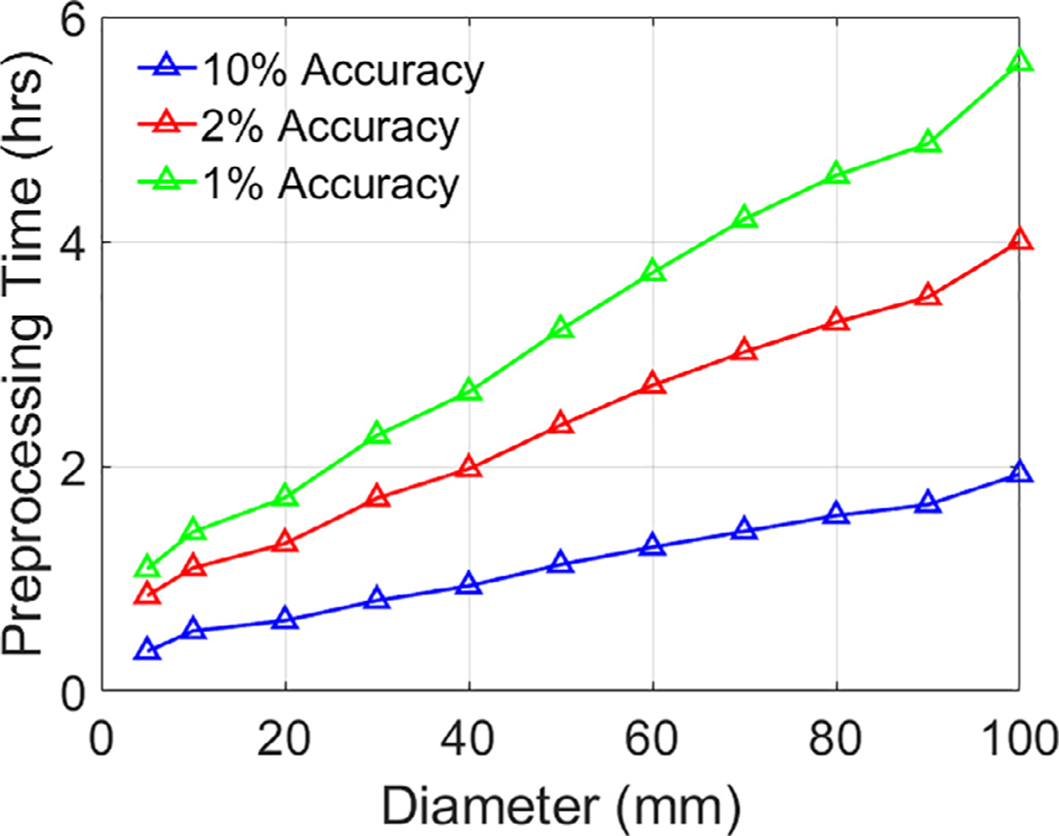
Averaged pre-processing CPU run-time cost versus ROI diameter for the Ernie head model.

A spherical head model and 10 MRI-derived head models are used in this study. The spherical head model consists of two concentric spherical compartments with inner and outer radii of 70 mm and 85 mm, respectively. As in Deng et al. (2013), we assign a single conductivity of 0.33 S/m to both spherical compartments. The ‘Ernie’ head model included in SimNIBS 3.2 was used for studying ROIs of varying sizes (Thielscher et al., 2015). For whole brain (gray and white) matter as ROIs, we considered additional MRI derived head models. The MRIs were downloaded from the following public database (Gorgolewski et al., 2017). These T1 and T2 images were converted to head models using SimNIBS ‘mri2mesh’ tool, which combines outputs from FreeSurfer (Reuter et al., 2012) and FSL (Jenkinson et al., 2012) and Gmsh (Geuzaine and Remacle, 2009) to generate a head model. On average, a single head model consists of four million tetrahedra. All of the MRI-derived head models consist of five homogeneous compartments such as GM, WM, cerebrospinal fluid (CSF), skull, and scalp. The respective conductivity values are set to 0.276 S/m, 0.126 S/m, 1.654 S/m, 0.01 S/m, and 0.465 S/m (Wagner et al., 2004). It took approximately 30–35 hours to generate a single head model using a single processor CPU. In this paper, we only consider the E-fields induced in the brain (i.e. GM and WM regions).

$$\begin{array}{l}\underset{¯}{\overline{ \mathbf{\text{Algorithm}}\hspace{0.17em}\mathbf{1}\hspace{0.17em}\text{Adaptive}\hspace{0.17em}\text{Cross}\hspace{0.17em}\text{Approximation}\hspace{0.17em}(\text{ACA}).\hspace{0.17em}\hspace{0.17em}\hspace{0.17em}\hspace{0.17em}\hspace{0.17em}\hspace{0.17em}\hspace{0.17em}\hspace{0.17em}\hspace{0.17em}\hspace{0.17em}\hspace{0.17em}\hspace{0.17em}\hspace{0.17em}\hspace{0.17em}\hspace{0.17em}\hspace{0.17em}\hspace{0.17em}\hspace{0.17em}\hspace{0.17em}\hspace{0.17em}\hspace{0.17em}\hspace{0.17em}\hspace{0.17em}\hspace{0.17em}\hspace{0.17em}\hspace{0.17em}\hspace{0.17em}\hspace{0.17em}}}\\ \text{Randomly}\hspace{0.17em}\text{initialize}\hspace{0.17em}{I}_1,{\tilde{\mathit{Z}}}^{\left(0\right)}=0,\mathit{R}=0,k=1. \\ 1.\hspace{0.17em}\text{Compute}\hspace{0.17em}\text{the}\hspace{0.17em}{I}_k^{th}\hspace{0.17em}\text{row}\hspace{0.17em}\text{of}\hspace{0.17em}\text{the}\hspace{0.17em}\text{residual}\hspace{0.17em}\text{error}: \\ \hspace{0.17em}\hspace{0.17em}\hspace{0.17em}\hspace{0.17em}\hspace{0.17em}\text{if}\hspace{0.17em}k=1,\\ \hspace{0.17em}\hspace{0.17em}\hspace{0.17em}\hspace{0.17em}\hspace{0.17em}\hspace{0.17em}{\mathit{R}}_{I_k,[:]}={\mathit{Z}}_{I_k,[:]};\\ \hspace{0.17em}\hspace{0.17em}\hspace{0.17em}\hspace{0.17em}\hspace{0.17em}\hspace{0.17em}\text{else}\\ \hspace{0.17em}\hspace{0.17em}\hspace{0.17em}\hspace{0.17em}\hspace{0.17em}{\mathit{R}}_{I_k,[:]}={\mathit{Z}}_{I_k,[:]}-\sum _{l=1}^{k-1}{\left({\mathit{u}}_l\right)}_{I_k}{\mathit{v}}_l.\\ 2.\hspace{0.17em}\hspace{0.17em}\text{Find}\hspace{0.17em}\text{the}\hspace{0.17em}{k}^{th}\hspace{0.17em}\text{column}\hspace{0.17em}\text{index:}\\ \hspace{0.17em}\hspace{0.17em}\hspace{0.17em}\hspace{0.17em}\hspace{0.17em}{J}_k=\mathit{argmax}\left\{{\mathit{R}}_{I_k,[:]}\right\}.\\ 3.\hspace{0.17em}\text{Compute}\hspace{0.17em}{\mathit{v}}_k\text{:}\hspace{0.17em}\\ \hspace{0.17em}\hspace{0.17em}\hspace{0.17em}\hspace{0.17em}\hspace{0.17em}{\mathit{v}}_k=\frac{{\mathit{R}}_{I_k,[:]}}{{\mathit{R}}_{I_k,{\mathit{J}}_k}}.\\ 4.\hspace{0.17em}\text{Compute} {\mathit{J}}_k^{th} \text{column}\hspace{0.17em}\text{of}\hspace{0.17em}\text{the}\hspace{0.17em}\text{residual}\hspace{0.17em}\text{error}\hspace{0.17em}\text{matrix:}\hspace{0.17em}\\ \hspace{0.17em}\hspace{0.17em}\hspace{0.17em}\hspace{0.17em}\hspace{0.17em}\text{if} k=1,\\ \hspace{0.17em}\hspace{0.17em}\hspace{0.17em}\hspace{0.17em}\hspace{0.17em}{\mathit{R}}_{[:],{\mathit{J}}_k}={\mathit{Z}}_{[:],{\mathit{J}}_k};\\ \hspace{0.17em}\hspace{0.17em}\hspace{0.17em}\hspace{0.17em}\hspace{0.17em}\text{then}\\ \hspace{0.17em}\hspace{0.17em}\hspace{0.17em}\hspace{0.17em}\hspace{0.17em}{\mathit{R}}_{[:],{\mathit{J}}_k}={\mathit{Z}}_{[:],{\mathit{J}}_k}-\sum _{l=1}^{k-1}{\left({\mathit{v}}_l\right)}_{{\mathit{J}}_k}{\mathit{u}}_l.\\ 5.\hspace{0.17em}\text{Compute} {\mathit{u}}_k: \\ \hspace{0.17em}\hspace{0.17em}\hspace{0.17em}\hspace{0.17em}\hspace{0.17em}{\mathit{u}}_k={\mathit{R}}_{[:],{\mathit{J}}_k}\\ 6.\hspace{0.17em}\text{Calculate}\hspace{0.17em}\text{the}\hspace{0.17em}\text{norms}\hspace{0.17em}\text{of}\hspace{0.17em}\text{the}\hspace{0.17em}\text{new}\hspace{0.17em}\text{approximate}\hspace{0.17em}\text{matrix:} \\ \hspace{0.17em}\hspace{0.17em}\hspace{0.17em}\hspace{0.17em}\hspace{0.17em}\text{if} k=1,\\ \hspace{0.17em}\hspace{0.17em}\hspace{0.17em}\hspace{0.17em}\hspace{0.17em}{‖{\tilde{\mathit{Z}}}^{\left(k\right)}‖}^2={‖{\tilde{\mathit{Z}}}^{\left(k-1\right)}‖}^2+{‖{\mathit{u}}_k‖}^2{‖{\mathit{v}}_k‖}^2.\\ \hspace{0.17em}\hspace{0.17em}\hspace{0.17em}\hspace{0.17em}\hspace{0.17em}\text{then}\\ \hspace{0.17em}\hspace{0.17em}\hspace{0.17em}\hspace{0.17em}\hspace{0.17em}{‖{\tilde{\mathit{Z}}}^{\left(k\right)}‖}^2={‖{\tilde{\mathit{Z}}}^{\left(k-1\right)}‖}^2+2\sum _{j=1}^{k-1}\left|{\mathit{u}}_j^T{\mathit{u}}_k\right|\cdot \left|{\mathit{v}}_j^T{\mathit{v}}_k\right|+{‖{\mathit{u}}_k‖}^2{‖{\mathit{v}}_k‖}^2.\\ 7.\hspace{0.17em}\text{Check}\hspace{0.17em}\text{convergence:}\hspace{0.17em}\\ \hspace{0.17em}\hspace{0.17em}\hspace{0.17em}\hspace{0.17em}\hspace{0.17em}\text{If}\\ \hspace{0.17em}\hspace{0.17em}\hspace{0.17em}\hspace{0.17em}\hspace{0.17em}‖{\mathit{u}}_k‖‖{\mathit{v}}_k‖\le ϵ‖{\tilde{\mathit{Z}}}^{\left(k\right)}‖,\\ \hspace{0.17em}\hspace{0.17em}\hspace{0.17em}\hspace{0.17em}\hspace{0.17em}\text{where} ϵ \text{is}\hspace{0.17em}\text{the}\hspace{0.17em}\text{pre-defined}\hspace{0.17em}\text{tolerance},\hspace{0.17em}\text{end}\hspace{0.17em}\text{iteration}.\hspace{0.17em}\text{Otherwise},\hspace{0.17em}\text{go} \\ \hspace{0.17em}\hspace{0.17em}\hspace{0.17em}\hspace{0.17em}\hspace{0.17em}\text{to}\hspace{0.17em}\text{next}\hspace{0.17em}\text{step}.\hspace{0.17em}\\ 8.\hspace{0.17em}\text{Find}\hspace{0.17em}\text{next}\hspace{0.17em}\text{row}\hspace{0.17em}\text{index:}\hspace{0.17em}\\ \underset{¯}{\hspace{0.17em}\hspace{0.17em}\hspace{0.17em}\hspace{0.17em}\hspace{0.17em}{I}_{k+1}=\mathit{argmax}\left|{\mathit{R}}_{[:],{\mathit{J}}_k}\right|.\hspace{0.17em}\hspace{0.17em}\hspace{0.17em}\hspace{0.17em}\hspace{0.17em}\hspace{0.17em}\hspace{0.17em}\hspace{0.17em}\hspace{0.17em}\hspace{0.17em}\hspace{0.17em}\hspace{0.17em}\hspace{0.17em}\hspace{0.17em}\hspace{0.17em}\hspace{0.17em}\hspace{0.17em}\hspace{0.17em}\hspace{0.17em}\hspace{0.17em}\hspace{0.17em}\hspace{0.17em}\hspace{0.17em}\hspace{0.17em}\hspace{0.17em}\hspace{0.17em}\hspace{0.17em}\hspace{0.17em}\hspace{0.17em}\hspace{0.17em}\hspace{0.17em}\hspace{0.17em}\hspace{0.17em}\hspace{0.17em}\hspace{0.17em}\hspace{0.17em}\hspace{0.17em}\hspace{0.17em}\hspace{0.17em}\hspace{0.17em}\hspace{0.17em}\hspace{0.17em}\hspace{0.17em}\hspace{0.17em}\hspace{0.17em}\hspace{0.17em}\hspace{0.17em}\hspace{0.17em}\hspace{0.17em}\hspace{0.17em}\hspace{0.17em}\hspace{0.17em}\hspace{0.17em}\hspace{0.17em}\hspace{0.17em}\hspace{0.17em}\hspace{0.17em}\hspace{0.17em}\hspace{0.17em}\hspace{0.17em}\hspace{0.17em}\hspace{0.17em}\hspace{0.17em}\hspace{0.17em}\hspace{0.17em}\hspace{0.17em}\hspace{0.17em}\hspace{0.17em}\hspace{0.17em}\hspace{0.17em}\hspace{0.17em}\hspace{0.17em}\hspace{0.17em}\hspace{0.17em}\hspace{0.17em}\hspace{0.17em}\hspace{0.17em}\hspace{0.17em}\hspace{0.17em}\hspace{0.17em}\hspace{0.17em}\hspace{0.17em}\hspace{0.17em}\hspace{0.17em}\hspace{0.17em}\hspace{0.17em}\hspace{0.17em}\hspace{0.17em}\hspace{0.17em}\hspace{0.17em}\hspace{0.17em}\hspace{0.17em}\hspace{0.17em}\hspace{0.17em}\hspace{0.17em}}\\ \end{array}$$

For both the spherical and MRI-derived head models, the ROIs are chosen as the gray and white matters contained in spherical regions with center r_ROI and diameter d_ROI. Figures of ROIs and detailed descriptions are given in the supplementary document. (Note: For sphere head results, here we used analytical methods used in Sarvas (1987) and Gomez et al. (2020) in lieu of ADM and FEM, respectively.) For the Ernie head model we generated a total of 3480 ROIs from all possible combinations of ${\mathit{d}}_{\mathit{ROI}}=\left\{5,10,\dots ,100\right\}$ mm and centered at 162 distinct locations as shown in the supplementary figures. The 162 ROI center locations were chosen projecting uniformly chosen points on the scalp to the cortex. This resulted in a uniform sample possible ROI centers on the brain. The uniformly chosen scalp positions where generated by first defining nearly uniform samples on the scalp by defining a 10–20 EEG system its surface and performing barycentric refinement to ensure dense and uniform coverage of the scalp. The cortical center locations of each of the 162 ROIs are provided in the supplemental material.

2.6. Benchmark metrics

To validate our method, we consider three metrics the stop criterion (M₁), ACA error (M₂), and SVD error. The stop criterion is defined as the approximation of the norm of the rank-1 update at each iteration as follows

$$M_1=\frac{‖{\mathit{u}}_k‖‖{\mathit{v}}_k‖}{‖{\tilde{\mathit{Z}}}^{\left(k\right)}‖},$$ (8)

where u_k, vk, ${\tilde{\mathit{Z}}}^{\left(k\right)}$are the column update, row update, and matrix approximation obtained during the k^th iteration of Algorithm 1, respectively.

The ‘ACA error’ is the relative Frobenius norm error of the residual defined as

$$M_2=\frac{‖\mathit{R}‖}{‖\mathit{Z}‖}=\frac{‖\mathit{Z}-{\tilde{\mathit{Z}}}^{\left(k\right)}‖}{‖\mathit{Z}‖}.$$ (9)

For all spherical head results and ROIs with diameter less than 30 mm, we compute M₂ exactly. For ROIs with sizes beyond 30 mm, M₂ is estimated by considering 128 random coil placements. For some examples, we additionally compute low-rank approximations using the SVD and compute the relative Frobenius norm error, which we term ‘SVD error’. The SVD is known to provide the optimal approximation for matrices (Trefethen and Bau III, 1997). As a result, this error represents the best possible error attainable for a rank-k approximation.

3. Results

3.1. Validation

Fig. 2 shows the errors obtained for ROIs with diameter of 10 mm and 20 mm in the spherical and Ernie head. For the spherical head, to achieve a 2% accuracy, the ACA (and SVD) required 6 (and 4) and 10 (and 6) iterations for the 10 mm and 20 mm diameter ROIs, respectively. For the MRI-derived head model, to achieve a 2% accuracy the ACA (and SVD) required 15 (and 7) and 17 (and 8) iterations for the 10 mm and 20 mm diameter ROIs, respectively. As expected, the ACA required a higher rank to achieve the same error as the SVD. Furthermore, this difference in rank for the same error becomes larger for larger ROIs. The SVD requires computation of the whole matrix, which requires either 180 (60 × 3) ADM runs to compute it row-wise or 346,680 (963 × 360) FEM runs to compute it column-wise for the smallest ROI of the four. The ACA avoids computing the matrix and requires exactly one ADM and FEM run per iteration. For all cases, the ACA required less than 2.15 times the rank of the SVD to reach a 2% accuracy, indicating that the computational time could nearly at most be halved using other matrix completion techniques for ROIs with diameter ≤ 20 mm. Fig. 3 shows exemplary E-field distributions in the 20 mm diameter ROIs of the spherical and Ernie heads. Both cases consist of the results from ACA-ADM and the reference results, obtained from analytical method in spherical head and from ADM in Ernie head. As expected, given the 2% relative error, the ROI E-fields are visually identical.

Fig. 2.

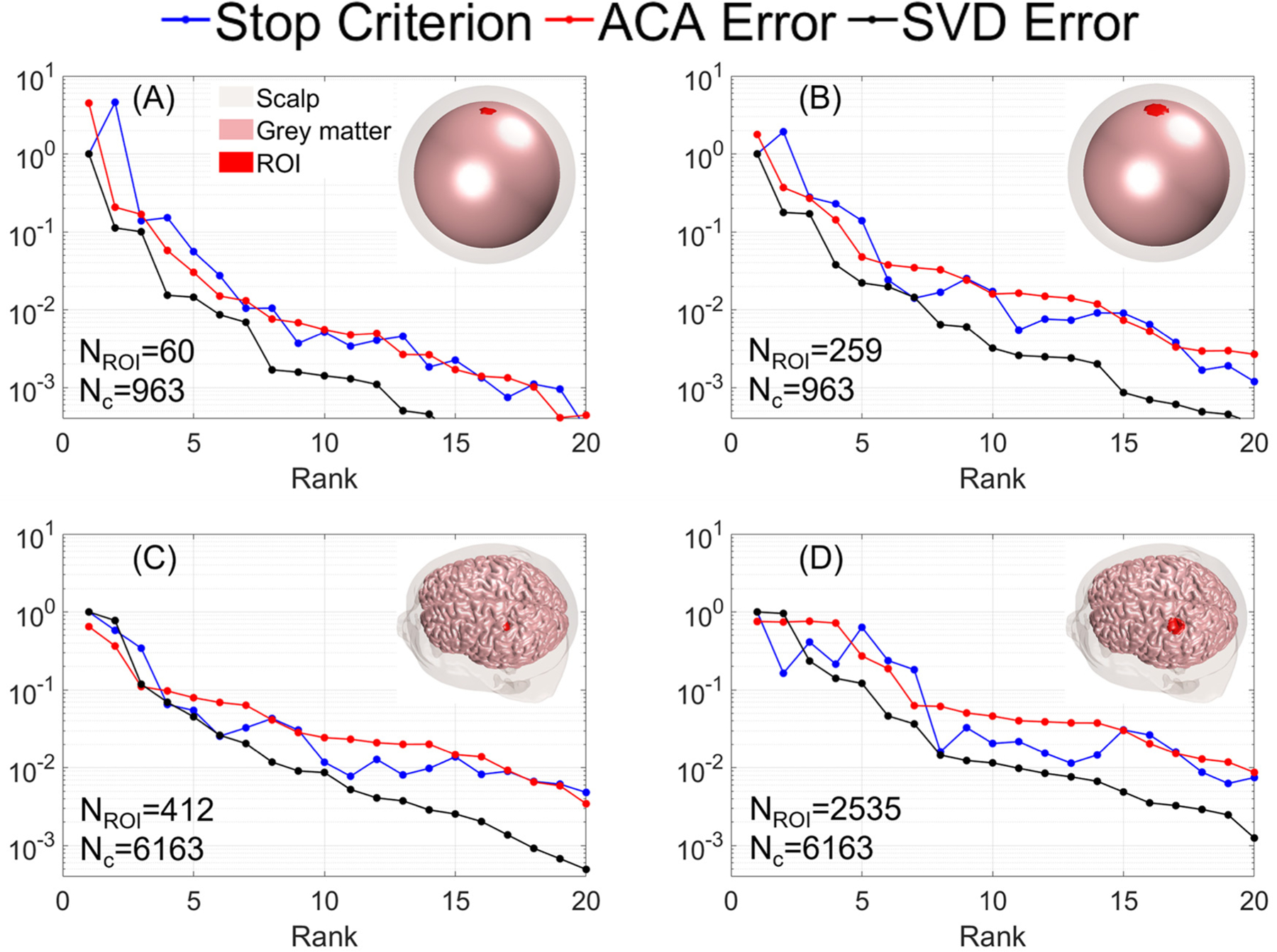
Convergence curves for each benchmark metric as a function of rank. (A) and (B) show the spherical head results for ROIs with diameters of 10 and 20 mm, respectively. (C) and (D) show the Ernie head results for ROIs with diameters of 10 and 20 mm, respectively.

Fig. 3.

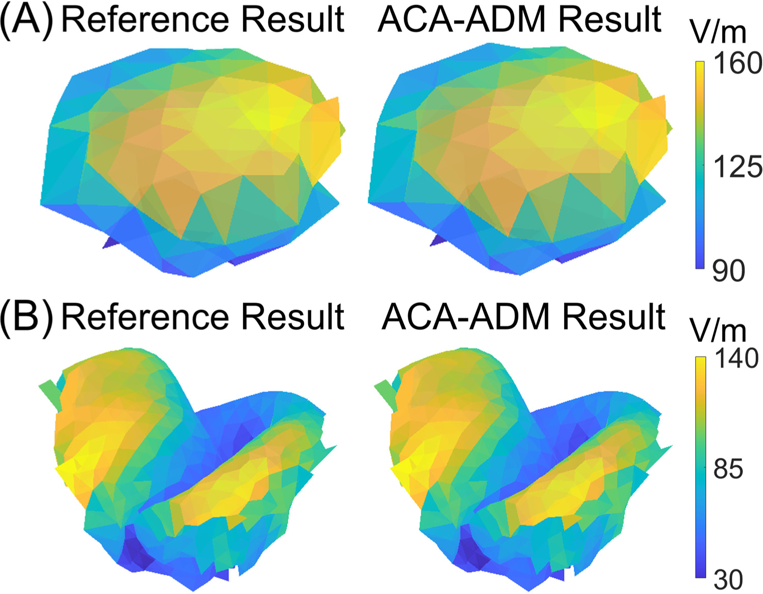
Exemplary E-field distributions computed using the reference and ACA-ADM method: (A) a 20 mm ROI result for the spherical head, and (B) a 20 mm ROI result for the Ernie head model.

In Fig. 2, the stop criterion for the ACA-ADM always follows the trend of the ACA error and thus indicative of the actual error. The rank to reach an ACA error and stop criterion level for ROIs of various diameters are shown in Fig. 4. The discrepancy between the ACA error and stop criterion increases with increasing accuracy level and ROI diameter.

Fig. 4.

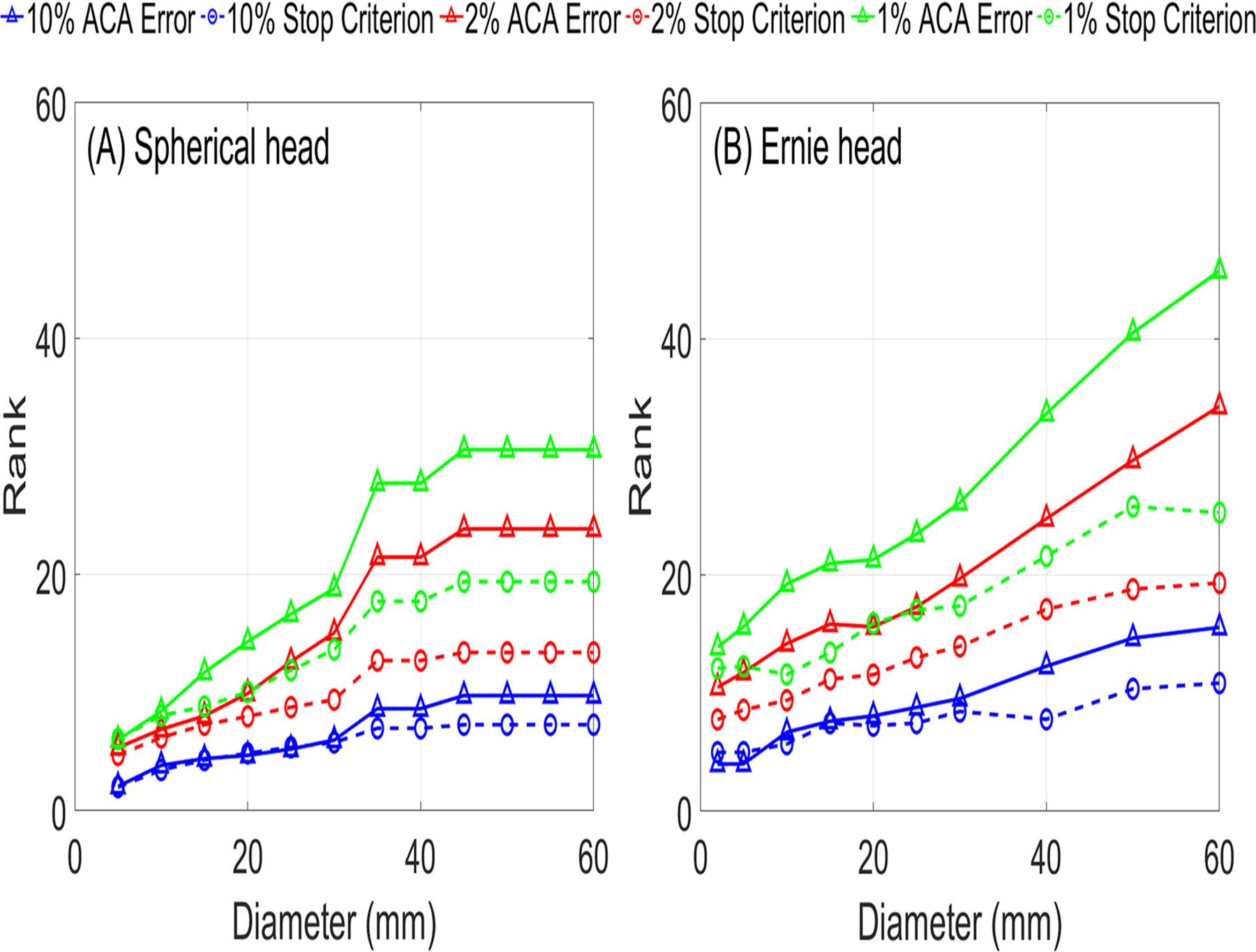
ACA rank required to achieve fixed accuracy levels versus ROI diameter for (A) the spherical and (B) Ernie head models.

To guarantee the robustness of the ACA algorithm, we further considered ROIs of varying sizes centered at 162 distinct locations as shown in the supplementary document. The statistical distributions of the maximum stop criteria and ranks required to achieve 10%, 2%, and 1% accuracy across all ROIs are shown in Fig. 5 and 6. If we chose a stop criterion that would guarantee a given accuracy across all ROIs, for many ROIs we would approximate the matrix to an accuracy much higher than required. More importantly, this would lead to slow convergence. In contrast, the number of iterations behaves less eratic across ROIs. Specifically, the number of iterations increases nearly linearly and monotonically with ROI diameter. To ensure robustness, we add an additional convergence criterion to the ACA based on a linear fit of the maximum rank required over all ROI diameters to achieve a given accuracy. Specifically, we run a fixed number of iterations before considering the ACA stop criterion. Additionally, we use a stop criterion equal to 0.25–0.5 times the required accuracy according to the ROI size.

Fig. 5.

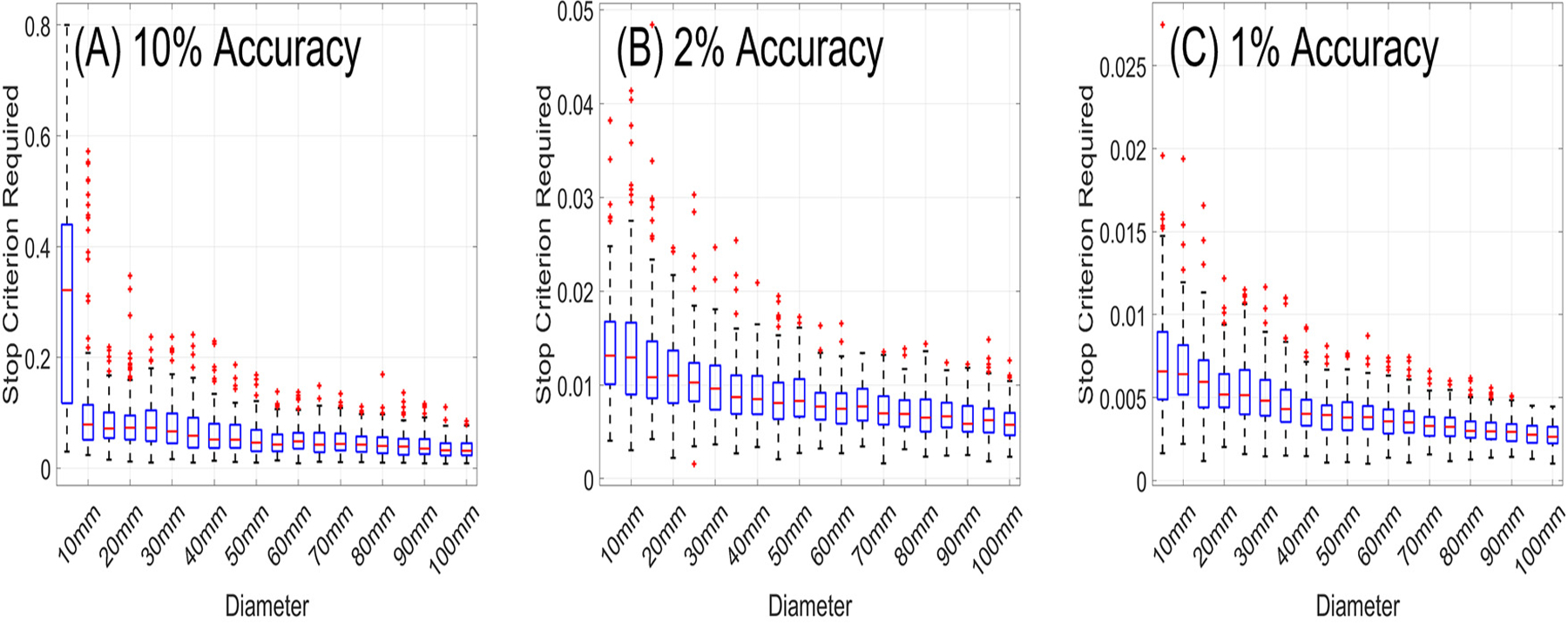
Statistical distributions for the maximum stop criterion required to achieve (A) 10% accuracy, (B) 2% accuracy, and (C) 1% accuracy.

Fig. 6.

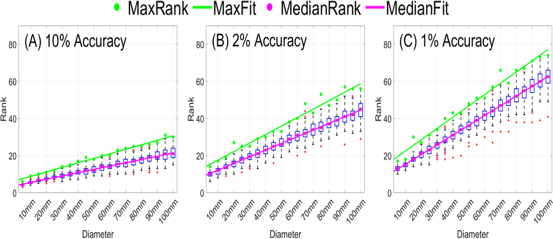
Statistical distributions of ranks required to achieve (A) 10% accuracy, (B) 2% accuracy, and (C) 1% accuracy and regressions for median and maximum rank. The magenta and the green points are the median and maximum rank, respectively. The solid lines are the regression lines.

We also considered the whole brain (gray and white) matter as ROI for 9 head models as shown in Fig. 7. We chose 21,358 to 25,895 nearly uniformly spaced coil positions (thus 7,688,880 to 9,322,200 coil placements) on the top of the scalp as shown in the supplemental document. The distributions of ranks to reach different levels of accuracy are shown in Fig. 7. To reach a 2% accuracy, the ranks ranged from 149 to 192. Therefore, for whole brain as ROI, we recommend setting the minimum rank as 200 to ensure convergence.

Fig. 7.

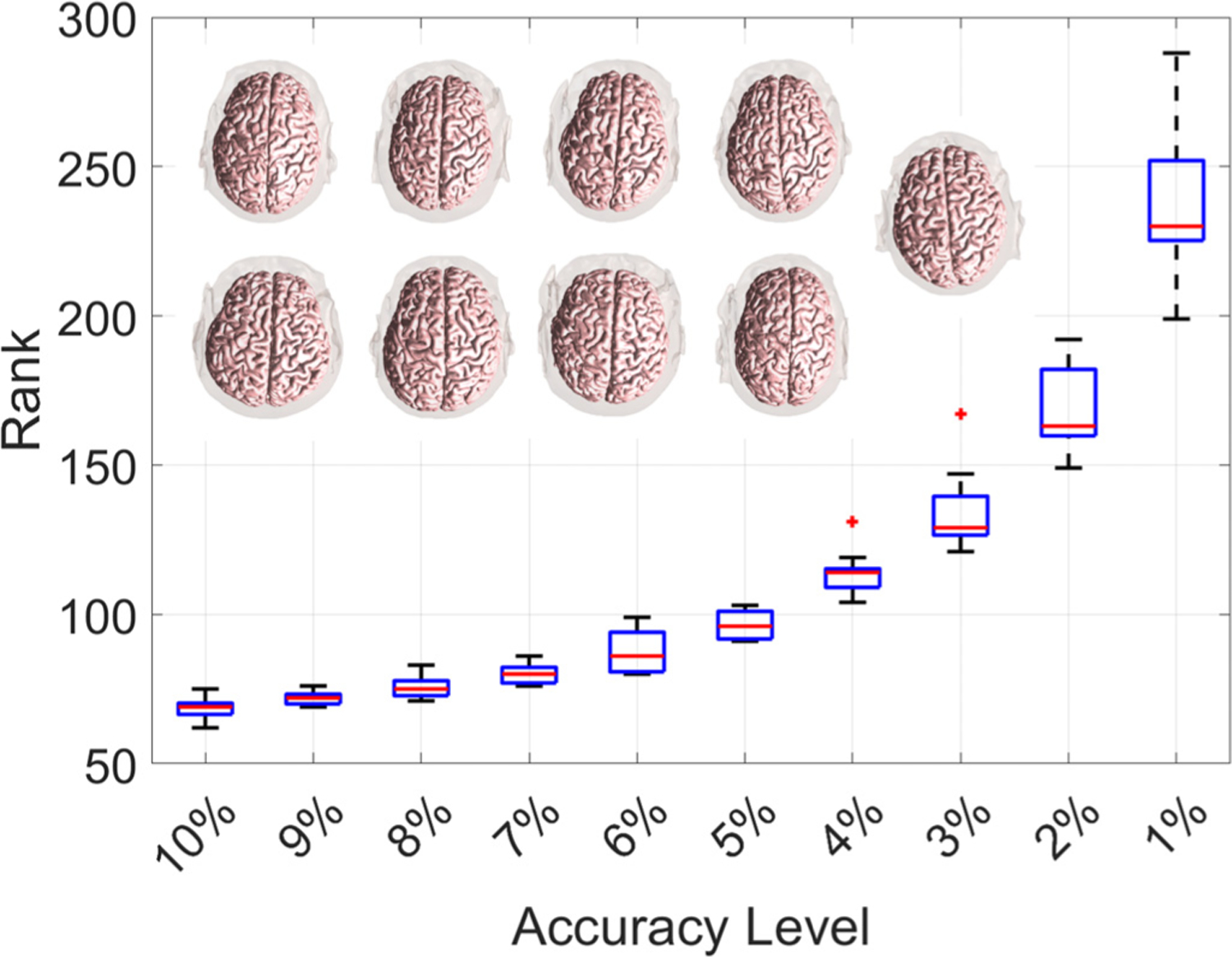
Distribution of ranks required to achieve a fixed accuracy level for the whole brain (gray and white) matter as ROI. The nine head models are shown within the figure as reference, and coil positions are provided in the supplemental document.

The pre-processing CPU run-time cost of the ACA-ADM for computing the coil placement (assuming N_c = 6163) to E-field matrix for different ROI diameters is shown in Fig. 8. For all cases, computing the matrix using FEM would have required 2,218,680 (6163 × 360) forward solves. Each forward solve on average takes 217 s, resulting in a total time of about 15.3 years. This could have been done using ADM, however, the number of ADM runs would grow with ROI size, because it would require 3N_t simulations, each taking approximately 105 s. For example, for ROIs with diameter of 20, 30, and 40 mm, it would require on average 5,316, 15,684, 33,908 simulations, respectively. In fact, for a small ROI with 20 mm diameter, the ACA method can construct the matrix with approximately 78 minutes whereas the ADM takes 9303 minutes. ADM is nearly 120 times slower than ACA-ADM even for this small example. For the ACA in contrast, the computation time per E-field sample grows sublinearly with ROI diameter because the rank grows slowly with increasing ROI size. Our results show that at most (i.e. for whole gray and white matters as ROIs) we need a rank of 192. In the supplement extended results of pre-processing and reconstruction times for whole brains are given. The pre-processing time to get a 2% accuracy ranged between 14.3 and 18.7 hours. The number of brain E-field samples ranged between 1.53 and 1.58 million, and, correspondingly, the reconstruction times ranged between 0.336 and 0.443 s on a CPU (2% accuracy). We also ran our simulations on an Nvidia GeForce RTX 3080 GPU and the reconstruction times ranged between 6.6 and 8.5 ms (2% accuracy).

CPU run-time is highly dependent on CPU architecture and comparisons across methods are best made using operation counts. Our reconstruction stage involves a dense matrix vector product, which is an embarrassingly parallel operation and easily optimized even for complicated CPU architectures. Here we provide CPU run-times for the processor mentioned in the introduction section for reference. The average time required for reconstructing E-field distributions for each ROI are shown in Fig. 9 (details of the reconstruction times for the 162 ROIs with different diameters are provided in supplemental document). The ACA-ADM can reconstruct an E-field distribution for a given coil placement in approximately 0.1 ms for a 20 mm ROI. Furthermore, it computes the E-field distribution in approximately 40 ms for ROIs with diameters less than 100 mm with a 2% accuracy.

Fig. 9.

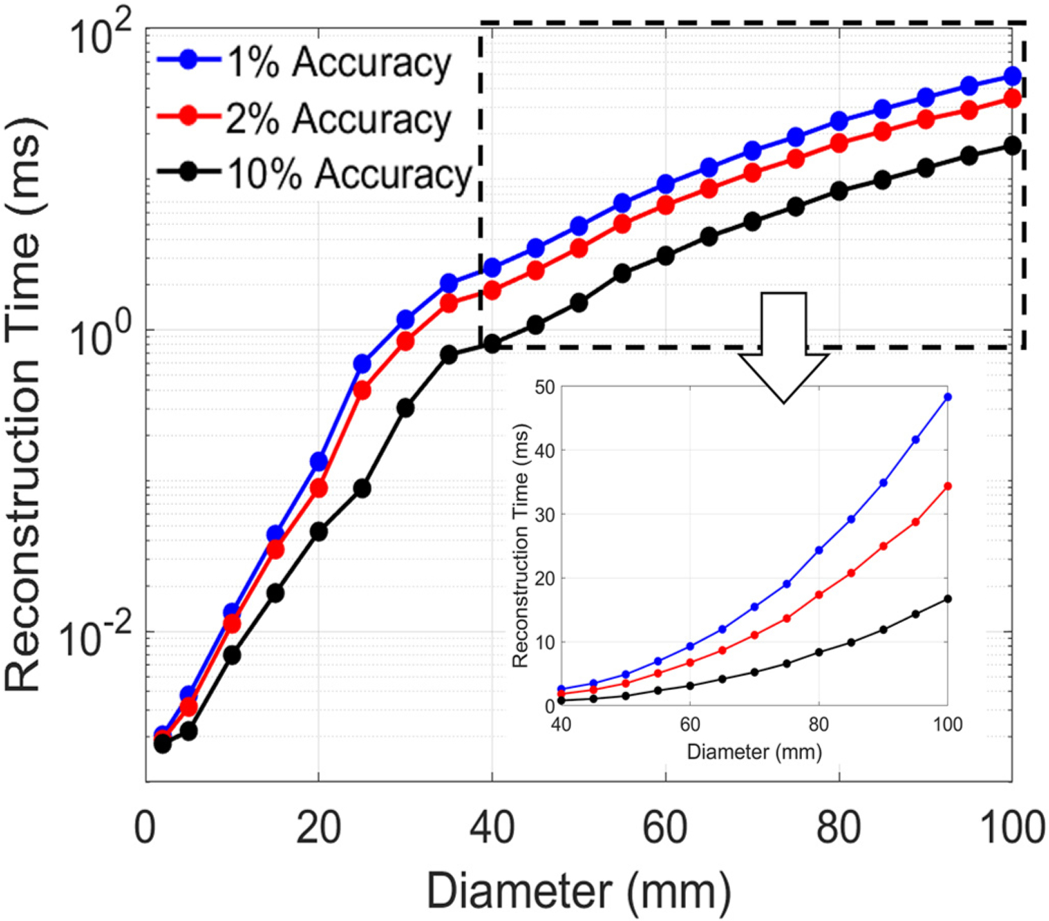
Averaged reconstruction time for the ROI E-field distribution computed by multiplying a column of V^(k) with U^(k).

3.2. Cortical motor mapping

Neuronavigated TMS (nTMS) is often used for cortical motor mapping for presurgical planning (Picht et al., 2013; 2011) and for neuroscience research (Salminen-Vaparanta et al., 2012). Neuronavigated TMS co-registers the subject’s head with MRI images and coil position(Ruohonen and Karhu, 2010). The position of the coil relative to the underlying cortical anatomy is then displayed along with E-field estimates. These E-field estimates are often derived from simplified spherical head models (Picht et al., 2011). During nTMS for cortical mapping, it is important to deliver a specified E-field to the targeted cortical sites (Krieg et al., 2017).

To illustrate the use of the ACA-ADM for nTMS, we computed E-field distribution in an ROI consisting of a long portion of the precentral gyrus as shown in Fig. 10 (A). The ROI has a diameter of 100 mm and consists of N_t=113,524 tetrahedra. The ACA-ADM took approximately 4.07 hours to generate the ROI E-field maps for 2,227,320 (6187 × 360) coil placements. Thereafter, the E-field maps could be computed in approximately 44 ms, indicating that the E-field could be overlayed on the ROI for nTMS in near real-time. Additionally, we computed the coil placement and orientation that generates a maximum E-field on different cortical sites along the precentral gyrus. These markers could be used to guide motor mapping procedures. This procedure can be extended to other cortical mappings, such as language mapping. Fig. 10 (B)-(I) show the E-field distribution as the coil moves along the scalp.

Fig. 10.

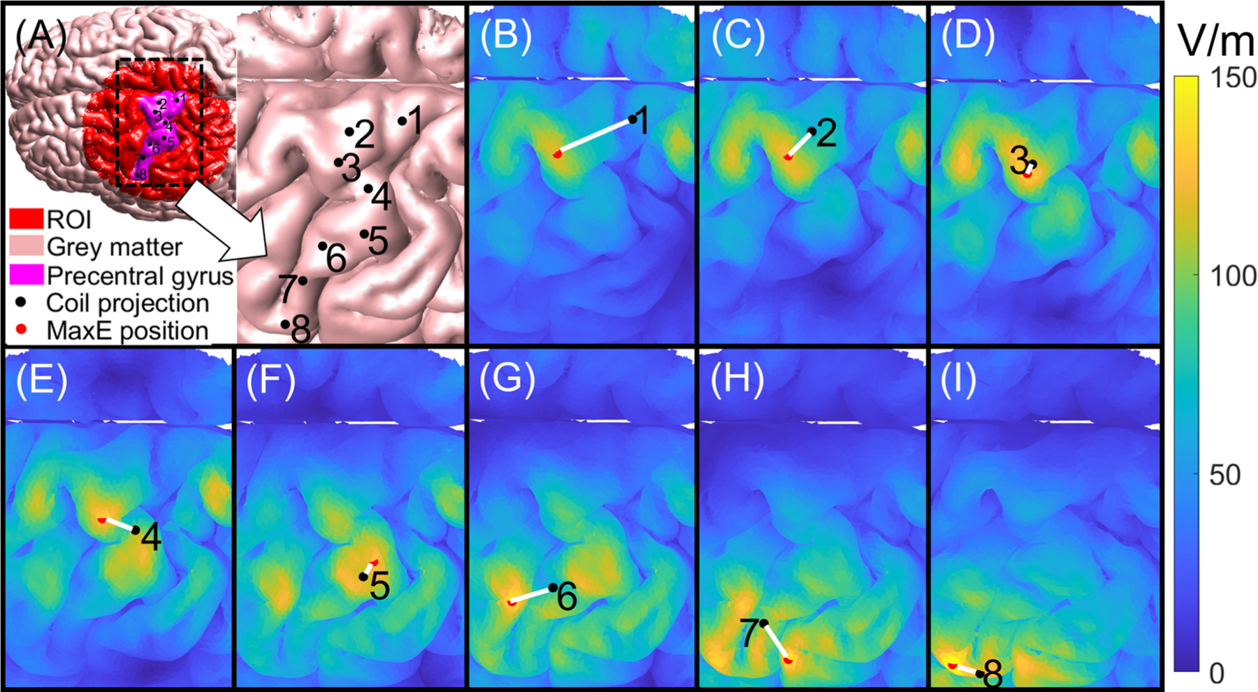
Cortical motor mapping example. (A) The head model and the coil projections on the precentral gyrus. (B)-(I) are the E-field distribution around the precentral gyrus. The black points are the coil projections on the cortex corresponding to the eight labels in (A), the red points are the brain positions with maximal E-field intensity, and the white line is the distance between the coil projection and the position with maximum E-field intensity.

3.3. Trade-off of on/off-target E-field exposure

Some TMS applications require inducing a large E-field on a specific ROI while minimizing it on specified ROIs. Here we illustrate how the ACA-ADM can be used to choose a coil placement to achieve the two objectives: Maximize E-field magnitude on the targetted ROI while minimizing it on the off-target ROI. Since this optimization has two objectives, we consider an objective function defined as

$${\mathit{E}}_M=\lambda {\mathit{E}}_R-{\mathit{E}}_G,$$ (10)

where ${\mathit{E}}_{R/G}$ are defined as the average E-field in the target/off-target ROIs, and λ determines the relative importance between E_R and E_G. A small λ prioritizes inducing a small E-field off target. As such, it results in coil placements far from both the target and off-target ROIs. In contrast, a large λ prioritizes maximizing target E-field, as such it results in coil placement that maximizes both target without suppressing off-target E-field.

Fig. 11 (A)-(C) shows the coil position for different values of λ. As we increase λ, the coil approaches the targeted site from the direction directly opposite to the off-target ROI. These coil placements both maximize the distance of the coil center to off-target ROI while minimizing the distance to the target ROI. In Fig. 11 (D)-(F), the average E-field for target and off target ROIs as a function of λ is shown. This information can be used to choose a coil placement that achieves a high enough E-field on the ROI while minimizing E-field on off-target region.

Fig. 11.

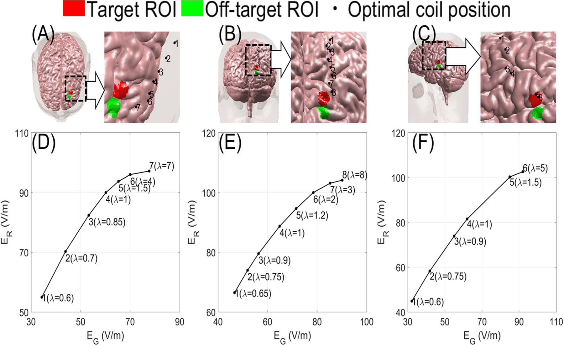
Maximizing target and minimizing off-target E-field. (A)-(C) The 10 mm diameter adjacent target (red) and off-target (green) ROIs on the frontal, occipital, and temporal lobe, respectively. (D)-(F) The average E-fields on-target and off-target ROIs as a function of λ on the frontal, occipital, and temporal lobe, respectively. The black points indicate optimal coil positions for the corresponding λ values in (D)-(F).

4. Discussion

Here we proposed a method for rapidly finding E-field distributions in brain ROIs. We showed the efficacy of this method in a variety of scenarios and possible applications of it. Our ACA-ADM approach works accurately and efficiently for any size ROI.

Since the ACA is a greedy algorithm, a small stop criterion value relative to the actual error can be observed at intermediate iterations. This could result in premature convergence and it is specially observed for large ROIs. From the spectral properties of Laplace’s equation, we know that the singular values of the coil placement to ROI E-field matrices will decay exponentially. Furthermore, we expect the rank for a fixed ROI size to be relatively fixed, as it is nearly only dependent on the scalp to cortex distance. As such, we proposed to fix the number of ACA iterations to ensure convergence.

Here we did not reduce the error below 1%. The rank required to further reduce the error in principle grows as logarithm because of the spectral properties of Laplace’s equation. That said, the FEM matrix only approximates the underlying physics. We notice that the rank increases more rapidly for error levels lower than 1% than what is theoretically expected. This is likely because at 1% we have already more than saturated the numerical accuracy of the 1st order FEM method used here (Gomez et al., 2020). If a more precise match between ACA-ADM and FEM is required, it is recommended to use a higher resolution mesh and/or higher order method.

The ACA-ADM algorithm is established based on the idea that the coil placement to E-field distribution in the ROI can be viewed as a compressible matrix, and this matrix can be determined using matrix completion algorithm. Specifically, the method introduced here is agnostic to method used to determine the E-fields. Correspondingly, the highly optimized BEMs presented in Daneshzand et al. (2021); Stenroos and Koponen (2019) could also be used in conjunction to the ACA in a non-intrusive manner to develop fast real-time E-field solver. Additionally, coil placements can be chosen on every node of the scalp triangle mesh and table entries interpreted as linear nodal element expansion coefficients, thereby, enabling its use to determine the E-field for any coil placement that is tangent to the scalp.

Validation results have shown that for both spherical head model and MRI-derived head model, the coil placement to ROI E-field distribution map compressed from just a few FEM and ADM runs. For example, for a typical ROI with diameter of 20 mm with 6163 coil positions, 17 FEM and 17 ADM runs are required by the ACA-ADM approach. This is in contrast to 5316 and 2,218,680 (6163 × 360) for ADM and FEM, respectively. Furthermore, the number of simulations required by the ACA-ADM increases slowly with the ROI size.

The ACA-ADM can be used for determining E-fields for both tangential and non-tangential coil placements outside of the head. The only constraint is that as the number of coil placements increases, the FEM run-time asymptotically increases linearly. This is because the ADM must compute the E-field for more coil positions. That said, results for the whole brain ROI had between 7.69 and 9.32 million coil placements, and the average single ACA run-time (including one FEM and one ADM run) is between 328 s and 354 s. Furthermore, the total pre-processing time was between 14.3 and 18.7 hours for a 2% accuracy. Additionally, the reconstruction time scales as the rank k times number of E-field samples in the brain and does not increase with increasing number of coil placements. For example, for the whole brain ROI results (with 1.53 to 1.58 million E-field sample locations) the reconstruction was at most 0.443 s on the CPU, and 8.5 ms on the GPU. This time is proportional to the number of E-field samples and can be reduced by choosing fewer E-field samples in the brain. These results indicate that for most applications the computational resource increases due to increased coil placements have minor practical consequences.

In this study we chose to place the coils tangentially because this is what is done in practice. However, ADM uses an auxiliary grid to discretize coils, which currently only works for flat or nearly flat coils. This limits the applicability of this method to Figure-8 type coils. The ACA-ADM can achieve acceptable accuracy for any size ROI. However, as the size of the ROI increases, the algorithm becomes less efficient as the ranks increase (Fig. 6). This increases the pre-processing time as shown in Fig. 8. For the whole brain (gray and white) matter as ROI, the worst case tested required a rank of 192 to achieve a 2% accuracy. This rank needs to be further reduced to make this practical for large size ROIs. We recommend applying the ACA-ADM for small ROIs (≤ 100 mm). For whole head we have been developing a method based on probabilistic matrix decomposition that has been shown to achieve nearly optimal compression for many applications (Halko et al., 2011).

5. Conclusions

Real-time TMS E-field dosimetry can be achieved for ROIs with diameters between 2 mm and 100 mm using ACA-ADM on a CPU. These times could be further accelerated using GPUs. The ACA-ADM solver requires a pre-processing phase of approximately 4 hours (for ROIs with up to 100 mm diameter) to generate a factorized form for the E-field distribution in the ROI for approximately two million coil placements. Then, this factorized form can be used to access E-fields in less than 40 ms for an ROI of 100 mm diameter with 2% accuracy. This tool could be used in neuronavigated TMS and for general E-field informed coil placement.

Data Availability

Data will be made available on request.

References

- Aberra AS, Wang B, Grill WM, Peterchev AV, 2020. Simulation of transcranial magnetic stimulation in head model with morphologically-realistic cortical neurons. Brain Stimul 13 (1), 175–189. [DOI] [PMC free article] [PubMed] [Google Scholar]
- Balderston NL, Roberts C, Beydler EM, Deng Z-D, Radman T, Luber B, Lisanby SH, Ernst M, Grillon C, 2020. A generalized workflow for conducting electric field–optimized, fmri-guided, transcranial magnetic stimulation. Nat Protoc 15 (11), 3595–3614. [DOI] [PMC free article] [PubMed] [Google Scholar]
- Bebendorf M, 2011. Adaptive cross approximation of multivariate functions. Constructive approximation 34 (2), 149–179. [Google Scholar]
- Bebendorf M, Rjasanow S, 2003. Adaptive low-rank approximation of collocation matrices. Computing 70 (1), 1–24. [Google Scholar]
- Beynel L, Davis SW, Crowell CA, Dannhauer M, Lim W, Palmer H, Hilbig SA, Brito A, Hile C, Luber B, et al. , 2020. Site-specific effects of online rTMS during a working memory task in healthy older adults. Brain Sci 10 (5), 255. [DOI] [PMC free article] [PubMed] [Google Scholar]
- Carmi L, Tendler A, Bystritsky A, Hollander E, Blumberger DM, Daskalakis J, Ward H, Lapidus K, Goodman W, Casuto L, et al. , 2019. Efficacy and safety of deep transcranial magnetic stimulation for obsessive-compulsive disorder: a prospective multicenter randomized double-blind placebo-controlled trial. American Journal of Psychiatry 176 (11), 931–938. [DOI] [PubMed] [Google Scholar]
- Casarotto S, Fecchio M, Rosanova M, Varone G, D’Ambrosio S, Sarasso S, Pigorini A, Russo S, Comanducci A, Ilmoniemi RJ, et al. , 2022. The rt-TEP tool: real-time visualization of TMS-evoked potentials to maximize cortical activation and minimize artifacts. J. Neurosci. Methods 370, 109486. [DOI] [PubMed] [Google Scholar]
- Cohen SL, Bikson M, Badran BW, George MS, 2022. A visual and narrative time-line of US FDA milestones for transcranial magnetic stimulation (TMS) devices. Brain Stimulation: Basic, Translational, and Clinical Research in Neuromodulation 15 (1), 73–75. [DOI] [PMC free article] [PubMed] [Google Scholar]
- Couturier JL, 2005. Efficacy of rapid-rate repetitive transcranial magnetic stimulation in the treatment of depression: a systematic review and meta-analysis. Journal of Psychiatry and Neuroscience 30 (2), 83–90. [PMC free article] [PubMed] [Google Scholar]
- Daneshzand M, Makarov SN, de Lara LIN, Guerin B, McNab J, Rosen BR, Hämäläinen MS, Raij T, Nummenmaa A, 2021. Rapid computation of TMS-induced e-fields using a dipole-based magnetic stimulation profile approach. Neuroimage 237, 118097. [DOI] [PMC free article] [PubMed] [Google Scholar]
- Dannhauer M, Brooks D, Tucker D, MacLeod R, 2012. A pipeline for the simulation of transcranial direct current stimulation for realistic human head models using SCIRun/BioMesh3D. In: 2012 Annual International Conference of the IEEE Engineering in Medicine and Biology Society. IEEE, pp. 5486–5489. [DOI] [PMC free article] [PubMed] [Google Scholar]
- Dannhauer M, Huang Z, Beynel L, Wood E, Bukhari-Parlakturk N, Peterchev AV, 2022. TAP: targeting and analysis pipeline for optimization and verification of coil placement in transcranial magnetic stimulation. J Neural Eng 19 (2), 026050. doi: 10.1088/1741-2552/ac63a4. [DOI] [PMC free article] [PubMed] [Google Scholar]
- De Ridder D, De Mulder G, Menovsky T, Sunaert S, Kovacs S, 2007. Electrical stimulation of auditory and somatosensory cortices for treatment of tinnitus and pain. Prog. Brain Res 166, 377–388. [DOI] [PubMed] [Google Scholar]
- Deng Z-D, Lisanby SH, Peterchev AV, 2013. Electric field depth–focality tradeoff in transcranial magnetic stimulation: simulation comparison of 50 coil designs. Brain Stimul 6 (1), 1–13. [DOI] [PMC free article] [PubMed] [Google Scholar]
- Geuzaine C, Remacle J-F, 2009. Gmsh: a 3-d finite element mesh generator with built-in pre-and post-processing facilities. Int J Numer Methods Eng 79 (11), 1309–1331. [Google Scholar]
- Goetz SM, Deng Z-D, 2017. The development and modelling of devices and paradigms for transcranial magnetic stimulation. International Review of Psychiatry 29 (2), 115–145. [DOI] [PMC free article] [PubMed] [Google Scholar]
- Gomez LJ, Dannhauer M, Koponen LM, Peterchev AV, 2020. Conditions for numerically accurate TMS electric field simulation. Brain Stimul 13 (1), 157–166. [DOI] [PMC free article] [PubMed] [Google Scholar]
- Gomez LJ, Dannhauer M, Peterchev AV, 2021. Fast computational optimization of TMS coil placement for individualized electric field targeting. Neuroimage 228, 117696. [DOI] [PMC free article] [PubMed] [Google Scholar]
- Gomez LJ, Goetz SM, Peterchev AV, 2018. Design of transcranial magnetic stimulation coils with optimal trade-off between depth, focality, and energy. J Neural Eng 15 (4), 046033. [DOI] [PMC free article] [PubMed] [Google Scholar]
- Gomez-Tames J, Hamasaka A, Laakso I, Hirata A, Ugawa Y, 2018. Atlas of optimal coil orientation and position for TMS: a computational study. Brain Stimul 11 (4), 839–848. [DOI] [PubMed] [Google Scholar]
- Goreinov SA, Tyrtyshnikov EE, Zamarashkin NL, 1997. A theory of pseudoskeleton approximations. Linear Algebra Appl 261 (1–3), 1–21. [Google Scholar]
- Gorgolewski KJ, Durnez J, Poldrack RA, 2017. Preprocessed consortium for neuropsychiatric phenomics dataset. F1000Res 6. [DOI] [PMC free article] [PubMed] [Google Scholar]
- Greengard L, Gimbutas Z, 2012. FMM3D Software https://cims.nyu.edu/cmcl/fmm3dlib/fmm3dlib.html.
- Halko N, Martinsson P-G, Tropp JA, 2011. Finding structure with randomness: probabilistic algorithms for constructing approximate matrix decompositions. SIAM Rev 53 (2), 217–288. [Google Scholar]
- Hoffman RE, Gueorguieva R, Hawkins KA, Varanko M, Boutros NN, Carroll K, Krystal JH, et al. , 2005. Temporoparietal transcranial magnetic stimulation for auditory hallucinations: safety, efficacy and moderators in a fifty patient sample. Biol. Psychiatry 58 (2), 97–104. [DOI] [PubMed] [Google Scholar]
- Ilmoniemi RJ, Sarvas J, 2019. Brain Signals: Physics and Mathematics of MEG and EEG MIT Press. [Google Scholar]
- Jenkinson M, Beckmann CF, Behrens TE, Woolrich MW, Smith SM, 2012. Fsl. Neuroimage 62 (2), 782–790. [DOI] [PubMed] [Google Scholar]
- Kaptsan A, Yaroslavsky Y, Applebaum J, Belmaker RH, Grisaru N, 2003. Right prefrontal TMS versus sham treatment of mania: a controlled study. Bipolar Disord 5 (1), 36–39. [DOI] [PubMed] [Google Scholar]
- Koponen LM, Nieminen JO, Ilmoniemi RJ, 2015. Minimum-energy coils for transcranial magnetic stimulation: application to focal stimulation. Brain Stimul 8 (1), 124–134. [DOI] [PubMed] [Google Scholar]
- Koponen LM, Nieminen JO, Mutanen TP, Stenroos M, Ilmoniemi RJ, 2017. Coil optimisation for transcranial magnetic stimulation in realistic head geometry. Brain Stimul 10 (4), 795–805. [DOI] [PubMed] [Google Scholar]
- Krieg SM, Lioumis P, Mäkelä JP, Wilenius J, Karhu J, Hannula H, Savolainen P, Lucas CW, Seidel K, Laakso A, et al. , 2017. Protocol for motor and language mapping by navigated TMS in patients and healthy volunteers; workshop report. Acta Neurochir (Wien) 159 (7), 1187–1195. [DOI] [PubMed] [Google Scholar]
- Laakso I, Hirata A, 2012. Fast multigrid-based computation of the induced electric field for transcranial magnetic stimulation. Physics in Medicine & Biology 57 (23), 7753. [DOI] [PubMed] [Google Scholar]
- Lan L, Zhang X, Li X, Rong X, Peng Y, 2017. The efficacy of transcranial magnetic stimulation on migraine: a meta-analysis of randomized controlled trails. J Headache Pain 18 (1), 1–7. [DOI] [PMC free article] [PubMed] [Google Scholar]
- Lipton RB, Dodick DW, Silberstein SD, Saper JR, Aurora SK, Pearlman SH, Fischell RE, Ruppel PL, Goadsby PJ, 2010. Single-pulse transcranial magnetic stimulation for acute treatment of migraine with aura: a randomised, double-blind, parallel-group, sham-controlled trial. The Lancet Neurology 9 (4), 373–380. [DOI] [PubMed] [Google Scholar]
- Lynch CJ, Elbau IG, Ng TH, Wolk D, Zhu S, Ayaz A, Power JD, Zebley B, Gunning FM, Liston C, 2022. Automated optimization of tms coil placement for personalized functional network engagement. Neuron [DOI] [PMC free article] [PubMed]
- Makarov SN, Noetscher GM, Burnham EH, Pham DN, Htet AT, de Lara LN, Raij T, Nummenmaa A, 2019. Software toolkit for fast high-resolution TMS modeling. bioRxiv 643346.
- Makarov SN, Noetscher GM, Raij T, Nummenmaa A, 2018. A quasi-static boundary element approach with fast multipole acceleration for high-resolution bioelectromagnetic models. IEEE Trans. Biomed. Eng 65 (12), 2675–2683. [DOI] [PMC free article] [PubMed] [Google Scholar]
- Makarov SN, Wartman WA, Daneshzand M, Fujimoto K, Raij T, Nummenmaa A, 2020. A software toolkit for TMS electric-field modeling with boundary element fast multipole method: an efficient matlab implementation. J Neural Eng 17 (4), 046023. [DOI] [PubMed] [Google Scholar]
- Nahas Z, Kozel FA, Li X, Anderson B, George MS, 2003. Left prefrontal transcranial magnetic stimulation (TMS) treatment of depression in bipolar affective disorder: a pilot study of acute safety and efficacy. Bipolar Disord 5 (1), 40–47. [DOI] [PubMed] [Google Scholar]
- O’Reardon JP, Solvason HB, Janicak PG, Sampson S, Isenberg KE, Nahas Z, McDonald WM, Avery D, Fitzgerald PB, Loo C, et al. , 2007. Efficacy and safety of transcranial magnetic stimulation in the acute treatment of major depression: a multisite randomized controlled trial. Biol. Psychiatry 62 (11), 1208–1216. [DOI] [PubMed] [Google Scholar]
- Pascual-Leone A, Rubio B, Pallardó F, Catalá MD, 1996. Rapid-rate transcranial magnetic stimulation of left dorsolateral prefrontal cortex in drug-resistant depression. The Lancet 348 (9022), 233–237. [DOI] [PubMed] [Google Scholar]
- Picht T, Krieg SM, Sollmann N, Rösler J, Niraula B, Neuvonen T, Savolainen P, Lioumis P, Mäkelä JP, Deletis V, et al. , 2013. A comparison of language mapping by preoperative navigated transcranial magnetic stimulation and direct cortical stimulation during awake surgery. Neurosurgery 72 (5), 808–819. [DOI] [PubMed] [Google Scholar]
- Picht T, Schmidt S, Brandt S, Frey D, Hannula H, Neuvonen T, Karhu J, Vajkoczy P, Suess O, 2011. Preoperative functional mapping for rolandic brain tumor surgery: comparison of navigated transcranial magnetic stimulation to direct cortical stimulation. Neurosurgery 69 (3), 581–589. [DOI] [PubMed] [Google Scholar]
- Reuter M, Schmansky NJ, Rosas HD, Fischl B, 2012. Within-subject template estimation for unbiased longitudinal image analysis. Neuroimage 61 (4), 1402–1418. [DOI] [PMC free article] [PubMed] [Google Scholar]
- Rokhlin V, 1985. Rapid solution of integral equations of classical potential theory. J Comput Phys 60 (2), 187–207. [Google Scholar]
- Ruohonen J, Karhu J, 2010. Navigated transcranial magnetic stimulation. Neurophysiologie clinique/Clinical neurophysiology 40 (1), 7–17. [DOI] [PubMed] [Google Scholar]
- Salminen-Vaparanta N, Koivisto M, Noreika V, Vanni S, Revonsuo A, 2012. Neuronavigated transcranial magnetic stimulation suggests that area v2 is necessary for visual awareness. Neuropsychologia 50 (7), 1621–1627. [DOI] [PubMed] [Google Scholar]
- Sarvas J, 1987. Basic mathematical and electromagnetic concepts of the biomagnetic inverse problem. Physics in Medicine & Biology 32 (1), 11. [DOI] [PubMed] [Google Scholar]
- Saturnino GB, Madsen KH, Thielscher A, 2019. Electric field simulations for transcranial brain stimulation using fem: an efficient implementation and error analysis. J Neural Eng 16 (6), 066032. [DOI] [PubMed] [Google Scholar]
- Siebner HR, Funke K, Aberra AS, Antal A, Bestmann S, Chen R, Classen J, Davare M, Di Lazzaro V, Fox PT, et al. , 2022. Transcranial magnetic stimulation of the brain: what is stimulated?–a consensus and critical position paper. Clinical Neurophysiology [DOI] [PMC free article] [PubMed]
- Stenroos M, Koponen LM, 2019. Real-time computation of the TMS-induced electric field in a realistic head model. Neuroimage 203, 116159. [DOI] [PubMed] [Google Scholar]
- Thielscher A, Antunes A, Saturnino GB, 2015. Field modeling for transcranial magnetic stimulation: A useful tool to understand the physiological effects of TMS? In: 2015 37th Annual International Conference of the IEEE Engineering in Medicine and Biology Society (EMBC). IEEE, pp. 222–225. [DOI] [PubMed] [Google Scholar]
- Toschi N, Welt T, Guerrisi M, Keck ME, 2008. A reconstruction of the conductive phenomena elicited by transcranial magnetic stimulation in heterogeneous brain tissue. Physica Med 24 (2), 80–86. [DOI] [PubMed] [Google Scholar]
- Trefethen LN, Bau III D, 1997. Numerical linear algebra, Vol. 50. Siam. [Google Scholar]
- Wagner TA, Zahn M, Grodzinsky AJ, Pascual-Leone A, 2004. Three-dimensional head model simulation of transcranial magnetic stimulation. IEEE Trans. Biomed. Eng 51 (9), 1586–1598. [DOI] [PubMed] [Google Scholar]
- Weise K, Numssen O, Thielscher A, Hartwigsen G, Knösche TR, 2020. A novel approach to localize cortical TMS effects. Neuroimage 209, 116486. [DOI] [PubMed] [Google Scholar]
- Ying L, Biros G, Zorin D, 2004. A kernel-independent adaptive fast multipole algorithm in two and three dimensions. J Comput Phys 196 (2), 591–626. [Google Scholar]
- Yokota T, Maki T, Nagata T, Murakami T, Ugawa Y, Laakso I, Hirata A, Hontani H, 2019. Real-time estimation of electric fields induced by transcranial magnetic stimulation with deep neural networks. Brain Stimul 12 (6), 1500–1507. [DOI] [PubMed] [Google Scholar]
- Zhao K, Vouvakis MN, Lee J-F, 2005. The adaptive cross approximation algorithm for accelerated method of moments computations of EMC problems. IEEE Trans. Electromagn. Compat 47 (4), 763–773. [Google Scholar]
Associated Data
This section collects any data citations, data availability statements, or supplementary materials included in this article.
Supplementary Materials
Data Availability Statement