

Abstract
Spiking Neural Networks (SNNs) stand as the third generation of Artificial Neural Networks (ANNs), mirroring the functionality of the mammalian brain more closely than their predecessors. Their computational units, spiking neurons, characterized by Ordinary Differential Equations (ODEs), allow for dynamic system representation, with spikes serving as the medium for asynchronous communication among neurons. Due to their inherent ability to capture input dynamics, SNNs hold great promise for deep networks in Reinforcement Learning (RL) tasks. Deep RL (DRL), and in particular Proximal Policy Optimization (PPO) has been proven to be valuable for training robots due to the difficulty in creating comprehensive offline datasets that capture all environmental features. DRL combined with SNNs offers a compelling solution for tasks characterized by temporal complexity. In this work, we study the effectiveness of SNNs on DRL tasks leveraging a novel framework we developed for training SNNs with PPO in the Isaac Gym simulator implemented using the skrl library. Thanks to its significantly faster training speed compared to available SNN DRL tools, the framework allowed us to: (i) Perform an effective exploration of SNN configurations for DRL robotic tasks; (ii) Compare SNNs and ANNs for various network configurations such as the number of layers and neurons. Our work demonstrates that in DRL tasks the optimal SNN topology has a lower number of layers than ANN and we highlight how the state-of-art SNN architectures used in complex RL tasks, such as Ant, SNNs have difficulties fully leveraging deeper layers. Finally, we applied the best topology identified thanks to our Isaac Gym-based framework on Ant-v4 benchmark running on MuJoCo simulator, exhibiting a performance improvement by a factor of 4.4 over the state-of-art SNN trained on the same task.
Subject terms: Computer science, Software
Introduction
Spiking Neural Networks (SNNs) are often regarded as the third generation of Artificial Neural Networks (ANNs) because their functionality closely resembles that of the mammalian brain compared to previous generations. Also, it has been established that SNNs offer greater expressiveness compared to conventional ANNs1. Being their behavior based on a system of Ordinary Differential Equations (ODEs) which depict spiking neurons as dynamic systems, SNNs inherit temporal dimensionality, with neuron dynamics capable of encoding information in membrane potentials. Also, their event-based nature, where spikes serve as the medium for communication between neurons, potentially leads to low inference latency, which is suitable for real-time tasks. These features are particularly appealing in Reinforcement Learning (RL) tasks for robotics, in which an agent has to learn dynamically through direct interaction with their surroundings in real-time2,3. In this context, SNNs emerge as a promising solution for efficiently tackling such tasks4. Common benchmarks employed for this purpose include Cartpole and Ant. In these environments, a neural network learns to control the robot joints to achieve a specific objective. Previous studies focusing on SNN for robotic tasks adopted a conversion of the inputs from the continuum domain to the spiking one5,6 before feeding the network. From this point of view, an alternative approach that we consider in this work is to feed directly the continuous input to the network and let the first layer of the SNN convert it into spikes, thus letting the network learn the spike representation.
Within DRL, two primary algorithm families exist: off-policy and on-policy2. Off-policy algorithms leverage data collected from previous neural network policies (i.e. representing past experience). In contrast, on-policy algorithms base their learning solely on data generated by the current policy being evaluated2. For off-policy algorithms, every sample is randomly taken from a buffer of collected samples, called the experience memory. As a consequence, there is no temporal correlation between consecutive samples and the network should be reset at every sample. On the other side, on-policy algorithms use temporally consecutive samples. For this reason, to leverage SNN time correlation capabilities, with on-policy algorithms the network is not reset between samples.
As the field of SNNs in DRL is relatively recent, most of the work done uses off-policy methods not exploiting the full potential of SNNs7–20.
Another relevant aspect to be considered when bringing SNN to DRL is the training method. To circumvent the non-differentiable nature of spikes, conversion-based methods have been proposed, which involve converting pre-trained ANNs into SNNs with identical architectures21–23. However, these methods typically require a high number of timesteps to attain comparable performance, leading to significant inference latency and energy consumption, making them unattractive for real-time robotic tasks.
Conversely, direct training methods employ Surrogate Gradients (SG) and lead to lower latency inference compared to conversion-based methods24–26. By substituting the all-or-nothing gradients of the spike activity function with various shapes of SG, they allow for gradient backpropagation within a broader range of membrane potentials. At the same time, numerous efforts25,27–30 have been undertaken to mitigate the gradient vanishing or explosion problems typical of SNN direct training, to enhance its performance. As a consequence, direct training enables competitive performance under low latency, making them mature to be applied in real-time DRL tasks.
As a result, to explore the potential of SNN for DRL, direct SNN training using the on-policy method is desirable. Also, training efficiency is key to performing an effective network exploration and comparing SNN performance with the one achievable with ANN, so as to promote further SNN exploration and optimization. Today, simulator acceleration and multi-environment learning are key enabling technologies for DRL31,32. However, SNN training and inference in such an efficient framework are missing.
In this work, we filled this gap by developing a framework called SpikeGym33 for training SNNs using the Proximal Policy Optimization (PPO)34 algorithm, implemented with Isaac Gym32 on top of skrl35. This framework takes full advantage of the Isaac Gym features, namely full GPU pipeline and multi-environment training. Thanks to our framework, training an SNN agent in Ant (Isaac Gym) takes about 7 min instead of 3 h and 20 min as required by State-of-the-Art (SoA) implementation based on Ant-v4 (MuJoCo), enabling a suitable exploration of the behavior of the agent. To replicate just one specific use-case (Ant) from the two analyzed in this study, which involved 2400 Deep Reinforcement Learning (DRL) training sessions (30 different deep neural network configurations, each replicated 20 times, across two phases of training and inference, and using both ANN and SNN) with state-of-the-art technologies5 it would have required 333 days of simulation time on a GPU-accelerated workstation. However, the proposed framework reduced this time to just 11 and a half days, rendering the study more manageable and facilitating replication.
Further, by applying SNNs to both Cartpole and Ant tasks in the Isaac Gym simulator, we demonstrate that SNNs exhibit greater robustness than ANNs in Cartpole task. However, deeper SNN architectures (with more than one layer) experience performance drops of up to 5 when using more hidden layers (2–4) compared to a single layer. This limitation becomes particularly apparent in the Ant task, where ANNs outperform SNNs due to the task demand for deeper layer utilization, which SNNs struggle to leverage effectively even using a state-of-art direct training method36. To assess the generality of this behavior beyond DRL tasks, we explored the application of SNNs in a self-supervised learning task involving the reconstruction of multimodal signals. Our findings align with observations from DRL tasks, indicating that SNNs face difficulties with deeper layer utilization in complex scenarios. To the best of our knowledge, this is the first study directly comparing the performance of directly trained SNN and ANN in DRL, showing the inefficiencies in training deep SNN networks. Finally, we apply the learning rules found in our experiments to the Ant-v4 benchmark in MuJoCo37 showing an increase in performance of 4.4 compared to the state-of-the-art spiking network proposed for the same task5.
In summary, our work includes the following key contributions:
We introduce a new framework called SpikeGym, which is built on IsaacGym and skrl, enabling the training of SNNs using the state-of-the-art reinforcement learning algorithm PPO in minutes rather than hours by state-of-the-art frameworks.
We conduct a performance comparison between several network configurations trained with the PPO algorithm in two well-known environments: Cartpole and Ant. Our results demonstrate that SNN can perform complex tasks but with lower performance than ANN. The reason is that they struggle to fully leverage the advantages of deeper layers.
To assess the generality of the effect of the number of layers on the SNN performance, we further investigate this behavior in a multimodal tracking task, where the same pattern persists.
Finally, we apply our insights to the Ant-v4 environment and compare our results with state-of-the-art, demonstrating that our framework and approach outperform the current state-of-the-art by a factor of 4.4.
We believe that our study and the framework that we make openly available to the community will stimulate researchers to further explore and address the current advantages and limits of SNNs in DRL tasks, thereby expanding the application potential of neuromorphic computing in real-world tasks.
Related work
Since Spiking Neural Networks (SNNs) are inherently dynamic systems, they are particularly well-suited for addressing temporal problems, such as those encountered in reinforcement learning (RL). Several studies have leveraged SNNs for RL tasks. For instance, the authors in38–40 applied Spike-Timing-Dependent Plasticity (STDP)-based learning rules to solve three OpenAI Gym Atari games41, an arm control task, and a lane-keeping problem, respectively. Similarly, in42,43, the Cartpole environment with discrete actions was successfully tackled, while custom environments were addressed in38,44–46.
STDP has also proven effective in navigation and obstacle avoidance tasks, as demonstrated in18,47,48. In these studies, agents were trained using RL to navigate 2D environments (such as a 1000 800 pixel rectangle and an ellipse) while avoiding obstacles, using ultrasonic sensors. Additionally, STDP has been widely utilized in training SNNs for visual-based input tasks, such as classification problems involving MNIST or DVS-MNIST datasets49,50.
To address the limitations of applying STDP to more complex RL tasks, alternative training approaches have been explored. One approach involves training an Artificial Neural Network (ANN) and subsequently converting it into an SNN51. Another approach employs gradient-based training algorithms24. For example, the authors of12,52 trained an ANN using RL and then converted it into an SNN to solve OpenAI Gym games41. Similarly, in Ref.53, this methodology was applied to a navigation task using LiDAR input, and in Ref.54, the NengoDL training framework was utilized to perform an obstacle avoidance task with a drone using an event camera as input.
In Ref.15, the performance of an ANN, an SNN, and an SNN converted from an ANN was compared across 17 OpenAI Gym games. The results indicated that the SNN outperformed the ANN in 12 games, while the ANN outperformed the SNN in four games. In one game (Tennis), all three networks performed equally. Notably, the SNN converted from the ANN never outperformed the other models. As previously discussed, a converted SNN can at best match the performance of the original ANN, but it loses the temporal capabilities inherent to SNNs.
In Ref.55, the authors utilized a gradient-based training algorithm implemented with the SpyTorch tool56 to solve two OpenAI Gym games41, namely CartPole and Acrobot. The network was validated by running it on the Intel Loihi board57. To achieve this, the authors proposed a quantization-aware training algorithm to match the Loihi weight resolution and used the membrane potential in the last layer to select actions. In our work, we fully exploit the potential of SNNs by training them directly with backpropagation, avoiding the conversion between ANNs and SNNs.
In Ref.4, a novel training method was proposed where the gradient is accumulated during inference in the training phase and then applied to the network at the end of inference. This method was tested in two OpenAI Gym games41 and was specifically designed for recurrent SNNs. Furthermore, in Ref.5, the authors applied SNNs to a robotic task using Proximal Policy Optimization (PPO) with a continuous action space. They introduced a new encoding method to convert input from a continuous domain to a spike domain. However, due to limitations in their framework, they did not perform any Network Architecture Search (NAS) either to further optimize the neural networks or to understand how the behavior of the layers changes the performance of the neural network.
Finally, to improve the robustness and efficiency of SNNs, recent advances such as the Spike-based Nonlinear Information Bottleneck (SNIB) framework58, Spike-based Information Bottleneck with Learnable State (SIBoLS)59, and High-Order Spike-Based Information Bottleneck (HOSIB)60 have been proposed. The SNIB framework introduces strategies like Squared, Cubic, and Quartic Information Bottleneck (SIB, CIB, QIB) to compress spiking representations, significantly improving robustness and performance, especially under noisy conditions. Similarly, SIBoLS enhances SNNs’ robustness and energy efficiency by using a learnable membrane potential state for hidden information representation, making it effective in handling noise and reducing power consumption. HOSIB further advances SNN training by incorporating second-order (SOIB) and third-order (TOIB) strategies, achieving better generalization, robustness, and power efficiency, particularly in deeper networks like VGG9 and ResNet18.
Background
Reinforcement learning
Reinforcement Learning (RL) is a hot research area due to its potential to solve complex control and robotics tasks and its resemblance to human learning behavior2. Unlike supervised and unsupervised learning, RL is characterized by: (i) the absence of an oracle, (ii) sparse feedback, and (iii) data generated during training2. Figure 1 depicts a typical RL loop. In this loop, the agent interacts with the environment, resulting in changes within the environment based on the agent’s actions. Examples of agents include drones, cars, robots, humans, and neural networks, while the environment is everything surrounding the agent. RL often utilizes simulators to replicate the interactions between one or more agents and their environments. As illustrated in Fig. 1, the agent selects an action () through a policy function (), changing the environment according to a transition function. The environment then provides feedback through rewards () and updates the agent’s state ()2.
Fig. 1.
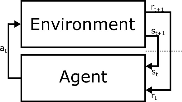
The reinforcement training loop involves the agent interacting with the environment: the agent takes an action , which causes the environment to evolve. The environment then provides the agent with the new state and the corresponding reward .
RL algorithms are categorized as follows:
Model-based or model-free;
Policy-based or value-based;
On-policy or off-policy.
Model-based algorithms aim to predict future observations and rewards, optimizing actions to achieve the goal. These algorithms are effective when the environment and its rules are well-defined, such as in chess RL applications61. Conversely, model-free algorithms do not construct a model of the environment, making them suitable for scenarios where the environment is either poorly understood or non-deterministic61. Policy-based algorithms focus on learning the action distribution the agent should follow at each step, while value-based algorithms assign scores to actions and select the highest-scoring one. Some algorithms combine both approaches, learning to score actions and determine their distribution. The distinction between on-policy and off-policy algorithms lies in the use of collected samples. On-policy algorithms train the agent using samples collected from the same policy being evaluated, whereas off-policy algorithms use samples collected from different policies61. In our work, we utilize the PPO algorithm, which is a model-free, combined method, and an on-policy algorithm. We chose PPO because it represents the state-of-the-art RL algorithms and, being on-policy, eliminates the need to reset the network after each sample.
PPO updates policies by taking the largest possible step to enhance performance while ensuring that the new and old policies remain within a specified range of similarity. This constraint is measured using KL-Divergence, a metric that quantifies the difference between two probability distributions. This approach differs from standard policy gradient methods, which maintain proximity between new and old policies in the parameter space. However, even minor changes in parameter space can lead to significant variations in performance, meaning that a single poorly chosen step can drastically degrade policy effectiveness. This risk necessitates small step sizes in traditional policy gradients, which, in turn, reduces sample efficiency. PPO effectively mitigates this risk by preventing such collapses and enabling rapid improvements in performance62.
PPO has two primary variants: PPO-Penalty and PPO-Clip. PPO-Penalty addresses the KL-constrained update by penalizing the KL-Divergence in the objective function rather than imposing it as a strict constraint. The algorithm automatically adjusts the penalty coefficient during training to ensure it is appropriately scaled. On the other hand, PPO-Clip does not include a KL-Divergence term or any explicit constraint. Instead, it relies on a specialized clipping mechanism in the objective function to prevent the new policy from straying too far from the old one62.
Among these, PPO-Clip is the most widely used variant. In this version, the neural network’s parameters (such as weights and biases) are updated according to the following equation:
| 1 |
where represents the states, the actions sampled from the old policy , and the parameters of the policies. Specifically, denotes the parameters of the new policy, are the ones in the previous policy, and represent the ones in a potential new policy. The objective function is defined as:
| 2 |
where is a small hyperparameter that restricts how much the new policy can diverge from the old one, is the advantage function, and is defined as:
| 3 |
Although this expression is complex, it effectively balances exploration and exploitation by keeping the new policy close to the old one. A simplified version of this objective, which is easier to understand and widely implemented in reinforcement learning libraries such as skrl, is given by:
| 4 |
Spiking neural networks
A Spiking Neural Network (SNN) consists of spiking neurons. Among the various neuron models proposed in the literature, the Leaky Integrate-and-Fire (LIF) model is one of the most widely used. The LIF model is described by the following equation:
| 5 |
where represents the time constant, v(t) denotes the membrane potential, R is the membrane resistance, and I(t) is the pre-synaptic current. For discrete-time algorithmic implementation, Eq. (5) can be reformulated recurrently, expressing the membrane potential at time as a function of the membrane potential at time t:
| 6 |
Here, dt is the integration step of the network simulation, referred to as a tick. The input current is defined by:
| 7 |
In this equation, n indicates the layer, j is the index of the pre-synaptic neuron, i is the index of the post-synaptic neuron, b is the bias (constant current), w are the synaptic weights, and z(t) are the spikes emitted by the neurons:
| 8 |
According to Eq. (8), a spike is generated if the membrane potential reaches the threshold during its rising phase.
Post-spike, the neuron can evolve in one of two ways depending on the design: (i) Resetting its v(t) to a fixed value called the resting membrane potential (hard-reset)24:
| 9 |
(ii) Subtracting the threshold from v(t) (soft-reset)4:
| 10 |
When the spiking behavior is disabled, the neuron operates as a “non-spiking LIF.” In our work, we employ both spiking and non-spiking LIF models with hard-reset behavior.
Encoding strategies
When working with Spiking Neural Networks (SNNs), converting continuous-domain inputs into spike-domain inputs is a critical task. The optimal strategy for this conversion remains an open research question, with three primary methods prevalent in the literature: (i) Rate-Coded Conversion (RCC), (ii) Delta Conversion (DC), and (iii) Latency-Coded Conversion (LCC)63
In Rate-Coded Conversion (RCC), information is encoded in the firing rate of neurons. For instance, consider a sample that needs to be converted into a rate-coded 3D tensor , where represents the number of time steps. Each feature of the original sample is encoded independently, with the normalized value (ranging from 0 to 1) serving as the probability of a spike occurring at any given time step63. This process can be modeled as a Bernoulli trial, where the spiking probability is :
| 11 |
By sampling from the Bernoulli distribution for each feature at every time step, the tensor is populated with 1’s and 0’s. For a gray-scale image, a pure white pixel () corresponds to a 100% probability of spiking, while a pure black pixel () will never generate a spike. A gray pixel with a value of will have an equal probability of producing either a “1” or a “0”. As the number of time steps increases, the proportion of spikes is expected to converge to 0.563. The limitation of this encoding method lies in its requirement for multiple time steps to achieve convergence and its dependence on bounded inputs (between 0 and 1). In RL tasks, where inputs’ boundaries are not known and rapid response is critical, the need for numerous time steps can introduce undesirable latency between the input and the actions generated by the SNN.
Delta Conversion (DC), on the other hand, generates spikes only in response to changes in the input signals, making it particularly effective for processing time-series data. However, if the input signal remains constant, no spikes are produced. This characteristic can be problematic in environments where the same input may represent different states, potentially leading to undesired behavior or even failure in robotic systems63.
Finally, Latency-Coded Conversion (LCC) focuses on the timing of spikes rather than the total number of spikes. In this approach, the temporal aspect of when a spike occurs carries the primary information. For example, a time-to-first-spike mechanism encodes a bright pixel as an early spike, whereas a dark input may spike later or not at all63. Unlike rate coding, latency encoding assigns significant importance to individual spikes, which is advantageous in control applications. Reducing the firing rate lowers both energy consumption and inference time in dedicated hardware, making this method particularly appealing for efficient, real-time control systems.
Spiking neural network training
Training Spiking Neural Networks (SNNs) is a challenging task due to the non-differentiability of the spike-generating function. To address this, several training methods have been developed, which can be categorized into three groups: (i) biologically accurate methods, (ii) hybrid methods, and (iii) gradient descent-based methods.
The first group includes methods based on Spike-Timing-Dependent Plasticity (STDP). These approaches face two main issues: they are typically limited to training shallow networks, and STDP primarily functions as a switch for synaptic connections, reducing the network’s expressiveness. Despite these limitations, STDP has been used in various tasks, such as semi-supervised MNIST classification50 and reinforcement learning tasks including simple obstacle avoidance with a LEGO robot47, lane-keeping problems40, and robotic arm control39.
The second group involves training an Artificial Neural Network (ANN) and then converting it into an SNN. NengoDL64 is a leading framework for this approach. This method has been applied to tasks such as obstacle avoidance54, autonomous driving using LiDAR53, and solving OpenAI Gym Atari games12,41. However, this approach does not fully exploit the expressive potential of SNNs, which is believed to be greater than that of ANNs1.
The third group employs backpropagation or its approximations to circumvent the training difficulties posed by the non-differentiable activation function of spiking neurons. Notable algorithms in this category include e-prop4, Spikeprop65, STBP24, and Slayer66. These methods have been successfully applied to image classification66,67, anomaly detection68, and reinforcement learning4,15,55.
A well-known training method in this group, Spatio-Temporal BackPropagation (STBP)24, addresses the non-differentiable spike function using various pseudo-derivative curves h(v):
| 12 |
| 13 |
| 14 |
| 15 |
where a is the peak width of the derivative. From top to bottom, these equations represent the derivatives of the rectangular function, polynomial function, sigmoid function, and Gaussian function, respectively24.
Methods
This section outlines the experimental framework employed in this work. We begin by introducing the architecture of the SpikeGym framework followed by the benchmark tasks used in the evaluation:
Cartpole (Fig. 2a) in Isaac Gym: This is a standard reinforcement learning benchmark focusing on balancing a pole.
Ant (Fig. 2b) in Isaac Gym: This task involves training a quadruped robot to achieve forward locomotion within the Isaac Gym environment.
Ant-v4 (Fig. 2c) in Mujoco: This is a similar quadruped locomotion task implemented within the MuJoco physics simulator.
Multimodal Tracking (Fig. 2d): This is a task in which the SNNs have to reconstruct a temporal signal.
To ensure reproducibility, we report in Table 1 a summary of the hyperparameters used throughout our work. We based our choices on32 for the ANNs & SNNs and the ANNs parameter sections while on our previous work8 for the SNNs section.
Fig. 2.

The four tasks that we use as a benchmark: (a) Cartpole (from32), (b) Ant (from32), (c) Ant-v4 (from37), (d) Multimodal tracking.
Table 1.
Hyperparameters.
| Parameters | Cartpole | Ant | Ant-v4 | Multimodal tracking | |
|---|---|---|---|---|---|
| ANNs & SNNs | Environments/dataset size | 512 | 4096 | 4096 | 512 train; 512 valid |
| Episode/sample length | / | 1000 | 1000 | 2000 | |
| Rollouts | 16 | 16 | 16 | – | |
| Batch size | – | – | – | 32 | |
| # Mini-batch | 1 | 2 | 2 | – | |
| Entropy loss scale | 0 | 0 | 0 | – | |
| Value loss scale | 2 | 1 | 1 | – | |
| Learning rate | 3e−04 | 3e−04 | 3e−04 | 1e−03 | |
| SNNs | Decay | 0.2 | 0.2 | 0.2 | 0.2 |
| Threshold | 0.5 | 0.5 | 0.5 | 0.5 | |
| Width peak | 0.5 | 0.5 | 0.5 | 0.5 | |
| Neurons | LIF | LIF | LIF | LIF | |
| Output neurons | No-Spiking LIF | No-Spiking LIF | No-Spiking LIF | No-Spiking LIF | |
| Ticks | 1 | 1 | 1 | 1 | |
| SG function | Rectangular | Rectangular | Rectangular | Rectangular | |
| ANNs | Neurons | ELU | ELU | ELU | – |
| Output neurons | Linear | Linear | Linear | – | |
SpikeGym architecture
Figure 3 shows the architecture of the SpikeGym framework we developed to enable accelerated training of DRL tasks using SNN-PPO. We built SpikeGym on top of skrl35 which is a well-known RL library, enabling our framework for both Nvidia Isaac Gym and MuJoCo37 simulators. To do so we extended the core classes of the skrl to enable SNN-PPO models.
Fig. 3.

SpikeGym comprises modifications to skrl to facilitate support for Spiking Neural Networks with PPO agents in Isaac Gym and MuJoCo environments. SpikeGym extends the internal skrl code to accommodate SNN-specific data, such as spike traces and membrane voltage, and enables the environment to handle the temporal dimension.
Our key modifications focused on the following components: PPO (src.agent.ppo): This module was modified to track both spiking activity and hidden states within the SNN. This involved implementing mechanisms for resetting the internal state and uploading data to memory during training. Memory (src.memory.base): The memory component was extended to handle the additional data streams required for SNN training. This includes retrieving hidden states and spike information alongside traditional observations. Neurons (src.neurons): We created a new module containing various spiking neuron implementations. This module provides options for commonly used neuron surrogate functions like Rectangular, Gaussian, and Sigmoid neurons. IsaacGymWrapper (src.wrapper): This wrapper was modified to return both input and output observations with an added temporal dimension, fitting to the temporal nature of SNNs. GymWrapper (src.wrapper): Similar to IsaacGymWrapper, modifications were made to handle temporal observations. BaseSNN (src.networks.base_snn): This new class enables the creation of SNNs based on user-provided YAML configuration files. The configuration file allows for specifying the SNN architecture and neuron types. ANN (src.networks.ann): A companion class (ANN) was created to facilitate the generation of ANNs using YAML configuration files. This allows for easy comparison between SNNs and ANNs performance on the same tasks.
By incorporating these modifications, SpikeGym offers a flexible and efficient framework for training SNN-PPO models within various simulated environments. The framework33 empowers researchers to explore the potential of SNNs for DRL tasks while leveraging the existing capabilities of skrl.
SNN-PPO architecture
This section outlines the neural network architectures used for both SNNs and ANNs. To ensure a fair comparison, both types of networks share the same overall Feed-Forward (FF) structure, as the tasks analyzed can be approximated using a Markov Decision Process (MDP).
The architecture comprises two main components: the shared feature extractor and the output heads. This structure is widely used in reinforcement learning tasks to accelerate the training process. The shared feature extractor is the initial stage, responsible for converting the input from the continuous domain into spikes and processing the state information. Rather than using a separate encoding layer, we use the first input layer for conversion in spikes. This again leads to a more fair comparison with ANN. In particular, for this study, we employed a variation of the LCC algorithm, as presented in4. Specifically, the inputs to the first layer—sensor readings—are treated as currents, which are then multiplied by the weights of the input layer. These input weights are considered parameters of the network and are updated during training to minimize the loss. Finally, we present the input only for one timestep.
The hidden layers’ configuration and the number of neurons were varied throughout our experiments to assess the impact of network complexity. After the shared feature extractor, the network branches into two separate output heads, each consisting of a single layer: (i) the action head, which predicts the optimal action for the agent in the current state, and (ii) the critic head, which estimates the value of the current state. By maintaining a consistent overall architecture, we aimed to isolate the influence of the spiking neuron implementation on performance, allowing for a more focused comparison where the primary difference lies in the neuron number and types and number of hidden layers.
We are addressing a reinforcement learning task, we aim to keep the number of ticks as low as possible to minimize the latency of the SNNs. In this study, we fixed the number of ticks at 1, hence the output firing rate alone is insufficient to capture the complexity of the environment8. To address this, we used No-Spiking LIF neurons as the output neurons.
Finally, to tackle the challenge posed by the non-differentiable nature of SNNs, which complicates their training, we employed a rectangular function with the hyperparameters listed in Table 1. This choice is based on previous studies8,24.
Isaac Gym
Isaac Gym32, developed by Nvidia, is a physics simulation environment specifically designed for robotics and control tasks. It excels in training and testing reinforcement learning algorithms. The core feature of Isaac Gym is its full GPU pipeline. This eliminates the bottleneck of data transfer between the CPU and GPU and enables the simultaneous simulation of multiple environments. Consequently, this feature significantly accelerates the training phase, leading to the development of more robust control policies in a shorter timeframe. In this work, we decide to analyze the neural networks in two well-known environments: Cartpole and Ant. In the MuJoCo37 simulator, these environments are widely used to test the RL algorithms and, since they are available in Isaac Gym, we decided to use them.
Cartpole
The Cartpole environment consists of a pole attached to a movable cart via a hinge joint. The state of the environment is typically represented by the angular positions and velocities of the pole and the cart. The objective in the Cartpole task is to balance the upright pole for as long as possible. This is achieved by defining a reward function that provides a positive reward for each timestep the pole remains balanced within a specific angular threshold. Conversely, negative rewards or termination of the episode might occur when the pole angle deviates beyond the threshold or the cart moves too far from the center position. Through reinforcement learning algorithms, the agent (controller) learns a policy that maps the observed state (pole and cart positions/velocities) to appropriate force actions applied to the cart. The goal of the policy is to maximize the accumulated reward by keeping the pole balanced for extended durations. In this task, we have an observation space composed of 4 observations and an output action space constituted of 1 action.
Ant
The Ant task features a flat, featureless ground plane where an ant robot interacts with the environment. The robot itself is a pre-defined quadruped model with actuated joints representing legs. The state of the environment is typically represented by the robot’s joint positions, velocities, and potentially sensor data like forces acting on its body parts. The primary objective in the Ant task is to maximize the forward speed of the ant robot. This is achieved by defining a reward function directly proportional to the robot’s forward velocity. As the robot moves faster, it accumulates a higher cumulative reward over time. Through reinforcement learning algorithms, the control policy for the ant is trained to utilize its available degrees of freedom (joint torques) to propel itself forward and maximize the accumulated reward. This learning process allows the policy to discover effective movement patterns for efficient locomotion. In this task, we have an observation space composed of 60 observations and an output action space constituted of 8 actions.
MuJoCo
The MuJoCo37 physics simulator offers a powerful platform for simulating robotic systems and evaluating control strategies. Unlike Isaac Gym, it does not leverage GPU parallel environment acceleration, hence the training takes longer.
Ant-v4
The Ant-v4 is a standard benchmark that is similar to Ant. However Ant-v4 features a distinct observation space containing 27 states, compared to the original Isaac Gym Ant’s observation space. Despite this variation, the action space remains the same, consisting of 8 actions. Notably, the reward function in Ant-v4 differs from the original Ant, even though both environments share the same objective of maximizing forward movement.
Multimodal tracking
This task aims to reconstruct temporal input signals lasting 20 seconds with a timestep of 0.01 seconds. SNN receives one timestep of the signal as input at each point in time and is tasked with reconstructing the corresponding timestep as its output. We chose to test the SNNs on this task because it closely resembles a reinforcement learning task. Similar to RL, the neural network must analyze a signal over time and reconstruct a new signal –though in this case, it reconstructs the same signal. The key difference is that here we use self-supervised training instead of RL.
The dataset for training and validation purposes consists of 512 samples each. The signals themselves are defined as the sum of 16 sinusoids described by the following equation:
| 16 |
where:
Amplitude: .
Frequency: .
Phase: .
Results
In this section, we first evaluate the SpikeGym training acceleration with respect to SoA RL SNN training tools, then we report a comparative analysis between ANNs and SNNs in two distinct DRL tasks in Isaac Gym: Cartpole and Ant, both in Isaac Gym. We further analyze the behavior of the same SNN configurations against an unsupervised non-RL multimodal tracking task to assess the generality of deeper SNN topologies.
Lastly, we apply the best network found thanks to SpikeGym to the Ant-v4 benchmark running in MuJoCo simulator to compare with a state-of-the-art SNN solving the same task37.
SpikeGym training acceleration
Recently released Nvidia Isaac Gym software32 promises to solve simulator acceleration issues by enabling multi-agent learning and parallel simulation on a full GPU pipeline. To support these features, we build, on top of skrl35, SpikeGym an SNN RL training framework to take advantage of GPU RL training acceleration leveraging Nvidia Isaac Gym. SpikeGym supports also the training in MuJoCo37 RL training framework used in SoA RL SNN training5. The runtime of all the experiments grouped by network architecture is in Table 2. With the former setup, we are able to run an SNN training algorithm in s i.e, about 7 min, against the s i.e., about 3 h and 20 min of SoA RL SNN training5, while a real-time Ant simulation, with the same amount of environments (4096) running in series, would have required about 6 days. Thanks to the speed-up of using the proposed framework with Isaac Gym, we can explore multiple architectures and hyperparameters and assess their behavior.
Table 2.
Runtime of the experiments.
| Network architecture | Cartpole | Ant | Ant-v4 | |||||||||
|---|---|---|---|---|---|---|---|---|---|---|---|---|
| Training (s) | Evaluation (s) | Training (s) | Evaluation (s) | Training (s) | Evaluation (s) | |||||||
| Mean | Std | Mean | Std | Mean | Std | Mean | Std | Mean | Std | Mean | Std | |
| [2] * 1 | 31.35 | 7.96 | 35.85 | 5.53 | 364.05 | 9.51 | 184.00 | 47.79 | – | – | – | – |
| [2] * 2 | 44.65 | 3.37 | 27.95 | 3.65 | 299.15 | 25.10 | 166.75 | 11.26 | – | – | – | – |
| [2] * 4 | 45.30 | 6.20 | 40.80 | 4.37 | 304.20 | 59.53 | 424.50 | 29.23 | – | – | – | – |
| [4] * 1 | 40.25 | 4.84 | 35.70 | 3.16 | 358.40 | 8.48 | 160.45 | 11.80 | – | – | – | – |
| [4] * 2 | 44.05 | 4.77 | 29.05 | 4.83 | 295.50 | 6.14 | 204.00 | 88.15 | – | – | – | – |
| [4] * 4 | 44.00 | 4.28 | 40.20 | 4.70 | 292.68 | 6.31 | 414.40 | 18.64 | – | – | – | – |
| [8] * 1 | 40.85 | 4.64 | 30.70 | 3.30 | 373.30 | 22.58 | 159.85 | 14.06 | – | – | – | – |
| [8] * 2 | 44.50 | 3.25 | 32.83 | 5.95 | 299.20 | 5.95 | 411.80 | 16.19 | – | – | – | – |
| [8] * 4 | 44.55 | 4.25 | 40.70 | 3.39 | 292.85 | 7.73 | 418.00 | 19.69 | – | – | – | – |
| [16] * 1 | 44.75 | 2.38 | 26.25 | 3.94 | 357.10 | 8.99 | 158.55 | 17.12 | – | – | – | – |
| [16] * 2 | 46.85 | 2.83 | 34.90 | 4.88 | 306.40 | 4.59 | 404.00 | 29.78 | – | – | – | – |
| [16] * 4 | 46.85 | 3.48 | 41.95 | 4.84 | 299.65 | 8.17 | 427.40 | 15.45 | – | – | – | – |
| [32] * 1 | 40.20 | 6.45 | 30.15 | 3.97 | 348.40 | 30.32 | 164.95 | 14.67 | – | – | – | – |
| [32] * 2 | 44.25 | 3.83 | 32.90 | 4.21 | 305.35 | 6.55 | 407.20 | 22.13 | – | – | – | – |
| [32] * 4 | 51.35 | 3.24 | 44.00 | 4.38 | 313.00 | 8.99 | 422.65 | 21.98 | – | – | – | – |
| [64] * 1 | 36.95 | 6.42 | 32.90 | 2.70 | 343.40 | 15.29 | 168.85 | 13.92 | – | – | – | – |
| [64] * 2 | 44.60 | 2.48 | 32.70 | 5.15 | 312.75 | 15.14 | 406.30 | 38.02 | – | – | – | – |
| [64] * 4 | 49.10 | 4.48 | 41.25 | 6.20 | 364.90 | 11.81 | 437.80 | 17.88 | – | – | – | – |
| [128] * 1 | 37.45 | 5.44 | 31.70 | 2.41 | 365.95 | 12.33 | 159.35 | 16.61 | – | – | – | – |
| [128] * 2 | 44.75 | 2.91 | 31.70 | 4.62 | 344.75 | 23.31 | 401.45 | 42.73 | – | – | – | – |
| [128] * 4 | 47.05 | 4.17 | 35.45 | 7.35 | 450.30 | 21.41 | 425.00 | 33.45 | – | – | – | – |
| [256] * 1 | 43.50 | 6.03 | 29.90 | 4.23 | 421.50 | 4.43 | 169.50 | 4.83 | – | – | – | – |
| [256] * 2 | 44.95 | 4.81 | 32.45 | 6.86 | 445.15 | 22.56 | 416.75 | 35.72 | – | – | – | – |
| [256] * 4 | 60.35 | 4.35 | 37.70 | 5.36 | 642.05 | 44.33 | 472.80 | 17.75 | – | – | – | – |
| [512] * 1 | 47.85 | 3.41 | 28.75 | 4.13 | 448.60 | 6.26 | 171.15 | 2.92 | 12 104.90 | 1509.36 | 11 054.05 | 458.07 |
| [512] * 2 | 53.70 | 4.23 | 31.55 | 6.30 | 643.20 | 50.28 | 420.95 | 42.93 | 11 831.70 | 465.60 | 11 621.60 | 776.31 |
| [512] * 4 | 83.00 | 5.86 | 34.10 | 5.53 | 1 072.55 | 99.10 | 515.80 | 69.64 | – | – | – | – |
| [1024] * 1 | 53.15 | 4.14 | 29.35 | 4.09 | 609.25 | 16.85 | 173.55 | 6.79 | – | – | – | – |
| [1024] * 2 | 75.15 | 4.74 | 30.30 | 3.95 | 1 133.60 | 113.40 | 491.00 | 61.05 | – | – | – | – |
| [2048] * 1 | 59.90 | 4.96 | 27.20 | 4.41 | 960.50 | 36.94 | 196.60 | 7.59 | – | – | – | – |
| Total | 47.84 | 11.27 | 33.70 | 6.68 | 459.96 | 238.18 | 313.56 | 135.10 | 11 970.25 | 1160.10 | 11,150.20 | 555.03 |
SNN-PPO applied to Cartpole task (DRL)
In this section, we describe the results achieved by both ANNs and SNNs in the Cartpole task performed in the Isaac Gym simulator. In this task, the best score the networks can reach is 512. In Fig. 4, we present the performance of different ANNs (left) and SNNs (right) in terms of median and first and third quantiles. On the y-axis, we represent the reward, while on the x-axis the architecture. Each experiment is conducted 20 times with 20 different seeds.
Fig. 4.

The plots depict the performance comparison between ANNs (left) and SNNs (right) in the Cartpole task, highlighting the median values along with the first and third quantiles. The y-axis represents the reward value, while the x-axis represents different network architectures (organized by: [ number of neurons per layer ] number of layers). Each experiment is repeated 20 times with 20 different seeds to ensure robustness and reliability of results.
Our analysis reveals that ANNs have a higher standard deviation compared to the SNNs counterparts, whose performance is more stable when the number of parameters allow the network to learn effectively (i.e. configurations from [64 1 and above). Considering the absolute performance, the best ANN reward is reached for deeper networks, featuring 2 and 4 layers, while the best SNNs are shallow networks (with 1 layer). Moreover, the figure depicts that ANNs tend to overfit for a smaller number of parameters, as evident from the drop in performance reached by ANNs featuring more than 128 neurons per layer. On the other hand, the SNNs tend to be more stable across architectures. While the performance degrades for deeper networks, SNN in this task can still exploit deeper layers, as 2 and 4-layer networks feature similar reward scores unless the number of neurons per layer is too low (below 64) or too high (more than 512).
Figure 5 reports the rewards of SNNs and ANNs relative to the number of parameters (i.e. weights and biases). Bars represent the quantiles, while dots represent the medians. The colors indicate the number of layers for each architecture: 1 is green, 2 is blue and 4 is purple. These results are plotted as a function of the parameters, reported on the x-axis. ANN results are reported on the left while SNNs are on the right. The plot shows that by fixing the number of parameters, ANN performs better with more layers. Indeed, considering networks with more than 100 parameters (we can consider the minimum amount of parameters to allow the network to learn properly), purple dots (4 layers) are always higher than blue and green dots (2 and 1 layers, respectively).
Fig. 5.

The plots depict the performance comparison between ANNs (left) and SNNs (right) in the Cartpole task, showcasing median values along with the first and third quantiles. The y-axis represents the reward value (the higher the better), while the x-axis represents the number of parameters (weights and biases). The colours represent the number of layers of each neural network. Each experiment is repeated 20 times with 20 different seeds to ensure robustness and reliability of results.
On the other side, SNNs show the opposite behavior: for a given number of parameters, the best performance is achieved with fewer layers. Indeed, green and blue dots (1 and 2 layers, respectively) are always better than purple dots (4 layers). Note that this behavior is accentuated when considering a more complex task such as Ant, as discussed in the following section. Overall, the performance of SNNs equalizes the one of ANNs, showing that, for this task, SNNs are a suitable approach, using a similar number of parameters and fewer layers this is probably due to the higher expressiveness of the spiking neurons.
The high variation observed in our experiments is attributed to the seed: each experiment was run 20 (as suggested in69) times with only the seed being varied. We opted for this approach because a well-known issue in reinforcement learning is the significant variation in performance caused by different seeds69–71. These results are aligned with the SoA. Finally, the best ANN and SNN are shown in Table 3.
Table 3.
Cartpole performance.
| Network type | # Hidden layers | Reward |
|---|---|---|
| ANN | 4 | 495.19 |
| SNN | 1 | 489.22 |
SNN-PPO applied to Ant task (DRL)
Figure 6 illustrates the performance of ANNs (left) and SNNs (right) in the Ant task of Isaac Gym. This task is characterized by a bigger number of both inputs and outputs than Cartpole. Also, the reward is defined as a more complex function of actions. Each experiment is conducted 20 times with 20 different seeds. The bars represent the quantiles, while the dots represent the median. As for Cartpole plots, colors here represent the number of layers: green, blue, and purple represent networks with one, two, and four layers respectively. With respect to the Cartpole case, the best ANN outperforms the best SNN configuration. However, similarly to Cartpole, the best ANN is a deeper network, as it is able to exploit a large number of parameters (–) by organizing them in 4 layers of neurons. On the other side, SNNs struggle to leverage deeper layers as it is not able to exploit more than – parameters, thus limiting their expressiveness with respect to ANNs counterparts.
Fig. 6.

The plots depict the performance comparison between ANNs (left) and SNNs (right) in the Ant task, showcasing median values along with the first and third quantiles. The y-axis represents the reward value (the higher the better), while the x-axis represents the number of parameters (weights and biases). The colours represent the number of layers of each neural network. Each experiment is repeated 20 times with 20 different seeds to ensure robustness and reliability of results.
The high variation observed in our experiments is attributed to the seed: each experiment was run 20 (as suggested in69) times with only the seed being varied. We opted for this approach because a well-known issue in reinforcement learning is the significant variation in performance caused by different seeds69–71. These results are aligned with the SoA. Finally, the best ANN and SNN are shown in Table 4.
Table 4.
Cartpole performance.
| Network type | # Hidden layers | Reward |
|---|---|---|
| ANN | 4 | 6371.29 |
| SNN | 1 | 5405.94 |
SNN-PPO applied to multimodal tracking task (unsupervised training)
The performance degradation observed by increasing the number of layers in SNN-PPO has been compared with SNN in unsupervised training. Specifically, SNNs have been trained for a non-RL task, namely Multimodal Tracking, where the task is to reconstruct a signal composed of a sum of 16 sinusoids. Each experiment is repeated 20 times with 20 different seeds. In Fig. 7, we report the performance, measured by mean loss, of various SNNs as a function of the number of parameters. SNNs have been trained using two different methods: SG (left) and a recent state-of-the-art training algorithm called LSG (right)36. We considered this alternative training method as it has shown to provide high accuracy in various image classification tasks, where SNNs are used in deep CNN topologies (Spiking-CNN, or SCNN). Note that the authors of this learning method did not report a study of performance as a function of the number of layers. As shown in Fig. 7, 1-layer networks consistently exhibit lower mean loss compared to 2- and 4-layer networks. Similar to the Cartpole task, Multimodal Tracking is relatively simpler than Ant, allowing deeper networks to still achieve acceptable performance. However, for both training algorithms, SNNs with a single layer outperform those with more layers, suggesting that the behavior observed in Cartpole and Ant is not specific to SNN-PPO. Instead, it appears to be an inherent characteristic of temporal tasks.
Fig. 7.

The plots depict the performance comparison between SG (left) and LSG (right) in the Multimodal Tracking task, showcasing median values along with the first and third quantiles. The y-axis represents the loss value (the lower the better), while the x-axis represents the number of parameters (weights and biases). The colours represent the number of layers of each neural network. Each experiment is repeated 20 times with 20 different seeds to ensure robustness and reliability of results.
Comparison against state-of-art SNN-PPO
In the Fig. 8, we compare the performance of the SNNs obtained using SpikeGym (green) against state-of-the-art SNNs (red)5, named PopSAN, applied to a DRL Ant-v4 task with PPO. To the best of our knowledge, this is the best SNN-PPO available in the literature. To perform a fair comparison, we first used SpikeGym to determine the best SNN configurations, then we applied it in the same simulation environment used in Ref.5, namely MuJoCo Advanced Physical Simulator. In particular, we considered SpikeGym networks with 1 and 2 layers and we compared with PopSAN network with the same number of layers.
Fig. 8.

Each boxplot represents the performance distribution of twenty experiments. Each experiment uses a different random seed. In green we have the results obtained with SpikeGym and an SNN configurated with two layers or one layer. In green, we have the results obtained with PopSAN.
On the y-axis, we show the rewards over 20 runs with 20 different seeds. Authors in Ref.5 use a hybrid ANN-SNN configuration, where their neural network is trained with an SNN as an actor and an ANN as a critic. They modeled the synapses and created a coder and decoder strategy in order to translate the continuous inputs into the spike domain. On the other side, our network is a full SNN (both actor and critic).
In Fig. 8 (left), experiments refer to Ant-v4 task in MuJoCo, where we show to compare the performance of 2 layers-deep PopSAN and SpikeGym networks. Results show that the SpikeGym SNN-PPO network features a median performance 1.8 higher than PopSAN. By considering the best SpikeGym network which has 1 layer, we observe that this outperforms both 1 layer and 2 layer-deep PopSAN network. In particular, in Fig. 8 (right) it is shown that 1 layer-deep SpikeGym reaches a 4.4 higher reward w.r.t. PopSAN. We can conclude that, in this case, one layer is all that is needed to obtain the best SNN-PPO performance.
Conclusions
In our study, we developed an SNN framework tailored for Deep Reinforcement Learning (DRL) using skrl and Isaac Gym, significantly reducing training time with respect to available tools. This framework facilitated a comprehensive comparison between ANNs and SNNs across two distinct RL tasks: Cartpole and Ant. Our findings revealed that: i) SNNs perform better with shallow networks compared to ANNs; ii) SNN is able to exploit deeper layers in simpler tasks, such as Cartpole and Multimodal Tracking. However, in more complex tasks, SNNs struggle to train these deeper layers, resulting in inferior performance compared to ANNs. We hypothesize that this behavior is linked to the surrogate gradient function, which approximates the gradient—resulting in greater inaccuracies as the SNN depth increases. This issue, along with coding strategies critical for effectively feeding information to SNNs, will be the focus of future investigation. Additionally, we observed that in simpler tasks such as Cartpole, SNNs achieved higher performance than ANNs with the same number of training parameters. This behavior is likely due to the greater expressiveness of spiking neurons compared to artificial neurons. Finally, leveraging insights gained from these experiments, we applied learned lessons to the Ant-v4 task, surpassing state-of-the-art algorithms by a factor of 4.4.
Author contributions
L.Z. formulated the main ideas, implemented the system, performed the experiments and data analysis and wrote the paper. F.B. contributed to the main ideas and performed data analysis. S.M. contributed to the experimental design and performed data analysis. S.T. performed data analysis and paper writing. A.B. contributed to the experimental design, performed data analysis, and paper writing. A.A. contributed to the main ideas and experimental design, performed data analysis and paper writing, and provided funding. All authors reviewed the manuscript.
Data availibility
The datasets generated and analysed during the current study are available in the SpikeGym repository or can be generated by running the code available in the same repository: https://gitlab.com/ecs-lab/spikegym.
Code availibility
Declarations
Competing interests
The authors declare no competing interests
Footnotes
Publisher’s note
Springer Nature remains neutral with regard to jurisdictional claims in published maps and institutional affiliations.
References
- 1.Maass, W. Networks of spiking neurons: the third generation of neural network models. Neural Netw.10, 1659–1671 (1997). [Google Scholar]
- 2.Keng, W. L. & Graesser, L. Slm lab. https://github.com/kengz/SLM-Lab (2017).
- 3.Hwangbo, J. et al. Learning agile and dynamic motor skills for legged robots. Sci. Robot.4, eaau5872 (2019). [DOI] [PubMed]
- 4.Bellec, G. et al. A solution to the learning dilemma for recurrent networks of spiking neurons. Nat. Commun.11, 1–15 (2020). [DOI] [PMC free article] [PubMed] [Google Scholar]
- 5.Tang, G., Kumar, N., Yoo, R. & Michmizos, K. Deep reinforcement learning with population-coded spiking neural network for continuous control. In Conference on Robot Learning, 2016–2029 (PMLR, 2021).
- 6.Chen, D., Peng, P., Huang, T. & Tian, Y. Fully spiking actor network with intralayer connections for reinforcement learning. IEEE Trans. Neural Netw. Learn. Syst. (2024). [DOI] [PubMed]
- 7.Shah, S., Dey, D., Lovett, C. & Kapoor, A. Airsim: High-fidelity visual and physical simulation for autonomous vehicles. In Field and Service Robotics (2017). arXiv:1705.05065.
- 8.Zanatta, L. et al. Directly-trained spiking neural networks for deep reinforcement learning: Energy efficient implementation of event-based obstacle avoidance on a neuromorphic accelerator. Neurocomputing562, 126885 (2023). [Google Scholar]
- 9.Zhang, D., Wang, Q., Zhang, T. & Xu, B. Biologically-plausible topology improved spiking actor network for efficient deep reinforcement learning. arXiv preprint[SPACE]arXiv:2403.20163 (2024).
- 10.Salvatore, N., Mian, S., Abidi, C. & George, A. D. A neuro-inspired approach to intelligent collision avoidance and navigation. In 2020 AIAA/IEEE 39th Digital Avionics Systems Conference (DASC), 1–9 (IEEE, 2020).
- 11.Zhang, D., Zhang, T., Jia, S. & Xu, B. Multi-sacle dynamic coding improved spiking actor network for reinforcement learning. Proc. AAAI Conf. Artif. Intell.36, 59–67 (2022). [Google Scholar]
- 12.Patel, D., Hazan, H., Saunders, D. J., Siegelmann, H. T. & Kozma, R. Improved robustness of reinforcement learning policies upon conversion to spiking neuronal network platforms applied to atari breakout game. Neural Netw.120, 108–115 (2019). [DOI] [PubMed] [Google Scholar]
- 13.Naya, K., Kutsuzawa, K., Owaki, D. & Hayashibe, M. Spiking neural network discovers energy-efficient hexapod motion in deep reinforcement learning. IEEE Access9, 150345–150354 (2021). [Google Scholar]
- 14.Oikonomou, K. M., Kansizoglou, I. & Gasteratos, A. A hybrid spiking neural network reinforcement learning agent for energy-efficient object manipulation. Machines11, 162 (2023). [Google Scholar]
- 15.Chen, D., Peng, P., Huang, T. & Tian, Y. Deep reinforcement learning with spiking q-learning. arXiv preprint[SPACE]arXiv:2201.09754 (2022).
- 16.Sun, Y., Zeng, Y. & Li, Y. Solving the spike feature information vanishing problem in spiking deep q network with potential based normalization. Front. Neurosci.16, 953368 (2022). [DOI] [PMC free article] [PubMed] [Google Scholar]
- 17.Tang, G., Kumar, N. & Michmizos, K. P. Reinforcement co-learning of deep and spiking neural networks for energy-efficient mapless navigation with neuromorphic hardware. In 2020 IEEE/RSJ International Conference on Intelligent Robots and Systems (IROS), 6090–6097. 10.1109/IROS45743.2020.9340948 (2020).
- 18.Mahadevuni, A. & Li, P. Navigating mobile robots to target in near shortest time using reinforcement learning with spiking neural networks. In 2017 International Joint Conference on Neural Networks (IJCNN), 2243–2250, 10.1109/IJCNN.2017.7966127 (2017).
- 19.Jiang, J. et al. Neuro-planner: A 3d visual navigation method for mav with depth camera based on neuromorphic reinforcement learning. IEEE Trans. Veh. Technol. (2023).
- 20.Walravens, M., Verreyken, E. & Steckel, J. Spiking neural network implementation on fpga for robotic behaviour. In Advances on P2P, Parallel, Grid, Cloud and Internet Computing: Proceedings of the 14th International Conference on P2P, Parallel, Grid, Cloud and Internet Computing (3PGCIC-2019) 14, 694–703 (Springer, 2020).
- 21.Hu, Y., Tang, H. & Pan, G. Spiking deep residual networks. IEEE Trans. Neural Netw. Learn. Syst. (2021). [DOI] [PubMed]
- 22.Kundu, S., Datta, G., Pedram, M. & Beerel, P. A. Spike-thrift: Towards energy-efficient deep spiking neural networks by limiting spiking activity via attention-guided compression. In Proceedings of the IEEE/CVF Winter Conference on Applications of Computer Vision, 3953–3962 (2021).
- 23.Wang, Z. et al. Towards lossless ANN-SNN conversion under ultra-low latency with dual-phase optimization. arXiv preprint[SPACE]arXiv:2205.07473 (2022).
- 24.Wu, Y., Deng, L., Li, G., Zhu, J. & Shi, L. Spatio-temporal backpropagation for training high-performance spiking neural networks. Front. Neurosci.12, 331 (2018). [DOI] [PMC free article] [PubMed] [Google Scholar]
- 25.Fang, W. et al. Deep residual learning in spiking neural networks. Adv. Neural. Inf. Process. Syst.34, 21056–21069 (2021). [Google Scholar]
- 26.Deng, S., Li, Y., Zhang, S. & Gu, S. Temporal efficient training of spiking neural network via gradient re-weighting. arXiv preprint[SPACE]arXiv:2202.11946 (2022).
- 27.Feng, L., Liu, Q., Tang, H., Ma, D. & Pan, G. Multi-level firing with spiking ds-resnet: Enabling better and deeper directly-trained spiking neural networks. arXiv preprint[SPACE]arXiv:2210.06386 (2022).
- 28.Guo, Y. et al. Recdis-snn: Rectifying membrane potential distribution for directly training spiking neural networks. In Proceedings of the IEEE/CVF Conference on Computer Vision and Pattern Recognition, 326–335 (2022).
- 29.Zheng, H., Wu, Y., Deng, L., Hu, Y. & Li, G. Going deeper with directly-trained larger spiking neural networks. Proc. AAAI Conf. Artif. Intell.35, 11062–11070 (2021). [Google Scholar]
- 30.Perez-Nieves, N. & Goodman, D. Sparse spiking gradient descent. Adv. Neural. Inf. Process. Syst.34, 11795–11808 (2021). [Google Scholar]
- 31.Musa, A., Zanatta, L., Barchi, F., Andrea, B. & Andrea, A. A method for accelerated simulations of reinforcement learning tasks of uavs in airsim. In SIMUL 22 (2022).
- 32.Makoviychuk, V. et al. Isaac gym: High performance gpu-based physics simulation for robot learning. arXiv preprint[SPACE]arXiv:2108.10470 (2021).
- 33.Zanatta, L. Spikegym. https://gitlab.com/ecs-lab/spikegym (2024).
- 34.Schulman, J., Wolski, F., Dhariwal, P., Radford, A. & Klimov, O. Proximal policy optimization algorithms. arXiv preprint[SPACE]arXiv:1707.06347 (2017).
- 35.Serrano-Muñoz, A., Chrysostomou, D., Bøgh, S. & Arana-Arexolaleiba, N. skrl: Modular and flexible library for reinforcement learning. J. Mach. Learn. Res.24, 1–9 (2023). [Google Scholar]
- 36.Lian, S. et al. Learnable surrogate gradient for direct training spiking neural networks. In Proceedings of the Thirty-Second International Joint Conference on Artificial Intelligence, IJCAI-23, 3002–3010 (2023).
- 37.Todorov, E., Erez, T. & Tassa, Y. Mujoco: A physics engine for model-based control. In 2012 IEEE/RSJ International Conference on Intelligent Robots and Systems, 5026–5033. 10.1109/IROS.2012.6386109 (IEEE, 2012).
- 38.Frémaux, N., Sprekeler, H. & Gerstner, W. Reinforcement learning using a continuous time actor-critic framework with spiking neurons. PLoS Comput. Biol.9, e1003024 (2013). [DOI] [PMC free article] [PubMed] [Google Scholar]
- 39.Tieck, J. C. V. et al. Learning target reaching motions with a robotic arm using dopamine modulated stdp. In 18th IEEE International Conference on Cognitive Informatics and Cognitive Computing (2019).
- 40.Bing, Z. et al. End to end learning of spiking neural network based on r-stdp for a lane keeping vehicle. In 2018 IEEE International Conference on Robotics and Automation (ICRA), 4725–4732 (IEEE, 2018).
- 41.Brockman, G. et al. Openai gym (2016). arXiv:1606.01540.
- 42.Lu, J., Hagenaars, J. J. & de Croon, G. C. Evolving-to-learn reinforcement learning tasks with spiking neural networks. arXiv preprint[SPACE]arXiv:2202.12322 (2022).
- 43.Liu, Y. & Pan, W. Spiking neural-networks-based data-driven control. Electronics12, 310 (2023). [Google Scholar]
- 44.Hazan, H. et al. Bindsnet: A machine learning-oriented spiking neural networks library in python. Front. Neuroinform.12, 89 (2018). [DOI] [PMC free article] [PubMed] [Google Scholar]
- 45.Yuan, M., Wu, X., Yan, R. & Tang, H. Reinforcement learning in spiking neural networks with stochastic and deterministic synapses. Neural Comput.31, 2368–2389 (2019). [DOI] [PubMed] [Google Scholar]
- 46.Chevtchenko, S. F. & Ludermir, T. B. Combining stdp and binary networks for reinforcement learning from images and sparse rewards. Neural Netw.144, 496–506 (2021). [DOI] [PubMed] [Google Scholar]
- 47.Lobov, S. A., Mikhaylov, A. N., Shamshin, M., Makarov, V. A. & Kazantsev, V. B. Spatial properties of stdp in a self-learning spiking neural network enable controlling a mobile robot. Front. Neurosci.14, 88 (2020). [DOI] [PMC free article] [PubMed] [Google Scholar]
- 48.Shim, M. S. & Li, P. Biologically inspired reinforcement learning for mobile robot collision avoidance. In 2017 International Joint Conference on Neural Networks (IJCNN), 3098–3105 (IEEE, 2017).
- 49.Paulun, L., Wendt, A. & Kasabov, N. A retinotopic spiking neural network system for accurate recognition of moving objects using neucube and dynamic vision sensors. Front. Comput. Neurosci.12, 42 (2018). [DOI] [PMC free article] [PubMed] [Google Scholar]
- 50.Diehl, P. U. & Cook, M. Unsupervised learning of digit recognition using spike-timing-dependent plasticity. Front. Comput. Neurosci.9, 99 (2015). [DOI] [PMC free article] [PubMed] [Google Scholar]
- 51.Rueckauer, B., Lungu, I.-A., Hu, Y., Pfeiffer, M. & Liu, S.-C. Conversion of continuous-valued deep networks to efficient event-driven networks for image classification. Front. Neurosci.11, 682 (2017). [DOI] [PMC free article] [PubMed] [Google Scholar]
- 52.Tan, W., Patel, D. & Kozma, R. Strategy and benchmark for converting deep q-networks to event-driven spiking neural networks. arXiv preprint[SPACE]arXiv:2009.14456 (2020).
- 53.Shalumov, A., Halaly, R. & Tsur, E. E. Lidar-driven spiking neural network for collision avoidance in autonomous driving. Bioinspir. Biomimet.16, 066016 (2021). [DOI] [PubMed] [Google Scholar]
- 54.Salvatore, N., Mian, S., Abidi, C. & George, A. D. A neuro-inspired approach to intelligent collision avoidance and navigation. In 2020 AIAA/IEEE 39th Digital Avionics Systems Conference (DASC), 1–9 (IEEE, 2020).
- 55.Akl, M., Sandamirskaya, Y., Walter, F. & Knoll, A. Porting deep spiking q-networks to neuromorphic chip loihi. Int. Conf. Neuromorphic Syst.2021, 1–7 (2021). [Google Scholar]
- 56.Neftci, E. O., Mostafa, H. & Zenke, F. Surrogate gradient learning in spiking neural networks: Bringing the power of gradient-based optimization to spiking neural networks. IEEE Signal Process. Mag.36, 51–63 (2019). [Google Scholar]
- 57.Davies, M. et al. Loihi: A neuromorphic manycore processor with on-chip learning. IEEE Micro38, 82–99 (2018). [Google Scholar]
- 58.Yang, S. & Chen, B. Snib: improving spike-based machine learning using nonlinear information bottleneck. IEEE Trans. Syst. Man Cybern. Syst. (2023). [DOI] [PubMed]
- 59.Yang, S., Wang, H. & Chen, B. Sibols: robust and energy-efficient learning for spike-based machine intelligence in information bottleneck framework. IEEE Trans. Cogn. Dev. Syst. (2023). [DOI] [PubMed]
- 60.Yang, S. & Chen, B. Effective surrogate gradient learning with high-order information bottleneck for spike-based machine intelligence. IEEE Trans. Neural Netw. Learn. Syst. (2023). [DOI] [PubMed]
- 61.Lapan, M. Deep Reinforcement Learning Hands-on (Packt Publishing, 2020).
- 62.Graesser, L. & Keng, W. L. Foundations of Deep Reinforcement Learning: Theory and Practice in Python (Addison-Wesley Professional, 2019).
- 63.Eshraghian, J. K. et al. Training spiking neural networks using lessons from deep learning. In Proceedings of the IEEE (2023).
- 64.Rasmussen, D. NengoDL: Combining deep learning and neuromorphic modelling methods. arXiv1805.11144, 1–22 (2018). [DOI] [PubMed]
- 65.Bohte, S. M., Kok, J. N. & La Poutré, J. A. Spikeprop: backpropagation for networks of spiking neurons. In ESANN, vol. 48, 419–424 (Bruges, 2000).
- 66.Shrestha, S. B. & Orchard, G. Slayer: Spike layer error reassignment in time. Adv. Neural Inf. Process. Syst.31 (2018).
- 67.Stromatias, E., Soto, M., Serrano-Gotarredona, T. & Linares-Barranco, B. An event-driven classifier for spiking neural networks fed with synthetic or dynamic vision sensor data. Front. Neurosci.11, 350 (2017). [DOI] [PMC free article] [PubMed] [Google Scholar]
- 68.Zanatta, L. et al. Damage detection in structural health monitoring with spiking neural networks. In 2021 IEEE International Workshop on Metrology for Industry 4.0 & IoT (MetroInd4. 0 &IoT), 105–110 (IEEE, 2021).
- 69.Henderson, P. et al. Deep reinforcement learning that matters. In Proceedings of the AAAI Conference on Artificial Intelligence, vol. 32 (2018).
- 70.Andrychowicz, M. et al. What matters in on-policy reinforcement learning? a large-scale empirical study. arXiv preprint[SPACE]arXiv:2006.05990 (2020).
- 71.Islam, R., Henderson, P., Gomrokchi, M. & Precup, D. Reproducibility of benchmarked deep reinforcement learning tasks for continuous control. arXiv preprint[SPACE]arXiv:1708.04133 (2017).
Associated Data
This section collects any data citations, data availability statements, or supplementary materials included in this article.
Data Availability Statement
The datasets generated and analysed during the current study are available in the SpikeGym repository or can be generated by running the code available in the same repository: https://gitlab.com/ecs-lab/spikegym.