Abstract
Machining optimization is crucial for determining cutting parameters that enhance machining economics. However, few studies address the significant variation in cutting tool wear and the complexities of discrete production, often leading to lower cutting parameters to prevent operational failures. Moreover, variations in part geometries lead to differing contact conditions between the cutting tool and workpiece, as well as variations in material removal. This study employs a robust optimization approach tailored for discrete workpieces to experimentally determine optimal cutting parameters that balance machining efficiency with cutting tool sustainability. An objective function was proposed to integrate tool wear probability and the number of workpieces, with case studies demonstrating its critical role in enhancing efficiency while achieving a tool overuse probability below 2.1 %. Our experiments reveal that processing either too few or too many parts with a single insert can escalate costs due to extreme tool wear or decreased efficiency; notably, the optimal number of parts to be machined was found to be four, yielding an objective function value of 380.6 NTD, which is lower than 394.5 NTD for three parts and 405.4 NTD for five parts in the case study. This research underscores the necessity of considering tool wear distribution and discrete production in machining optimization for sustainable manufacturing applications, providing valuable insights into the impact of cutting parameters and tool wear distribution on the costs for discrete production.
Keywords: Machining economics, Robust optimization, Integer optimization, Cutting tool sustainability, Tool wear distribution, Turning
1. Introduction
Cutting tool wear has been studied for over a century [1]; however, it remains a highly variable phenomenon and poses challenges in determining the optimal replacement time and avoiding production losses. Most studies have focused on continuous machining processes, with less attention given to discrete production. In discrete production, the part geometry is determined by specific requirements, and the cutting tool must last through the entire operation without significant wear or frequent replacement. Ideally, the tool should reach the end of its life only after completing the full operation or a specified number of operations, ensuring consistent cutting quality. As a result, the optimal cutting parameters vary based on different part designs and operations, an area that has been relatively underexplored. Metal cutting is influenced by various uncertainties, including the machine tool, clamping device, tooling, and the cutting process [2]. Experimental studies have shown that even in stable processes, cutting tool wear can have a standard deviation of up to 10 % of the mean value [3]. Therefore, cutting tools are often underused to prevent unacceptable surface quality, shock, and excessive vibration, which increases waste disposal and production costs [4]. However, the underutilization of cutting tools carries the risk of reducing their lifespan and wasting their potential usage. For affordable product prices and cost-effective production, continuous innovation and development in machining processes are necessary. Although the technologies such as coated cutting tools, minimum quantity lubrication, and spray cooling have been investigated to improve the cutting efficiency and sustainability [[5], [6], [7], [8], [9], [10]], the fine-tuning of cutting settings to manage tool wear effectively in the process is still crucial due to the use of diverse materials and intricate product design. A sustainable machining process for discrete production requires robust optimization that considers the variation in tool wear.
Selecting cutting parameters is a multifaceted process that depends on material removal rate, tool life, part quality, and associated machining costs. Good cutting parameters can reduce wasted operation time and cutting tools while maintaining the part quality. Therefore, optimization methods have been applied to find the optimum cutting parameters. Cakir and Gurarda evaluated the effect of constraints on the objective function using graphical representation, and the revised graph can be inspected for possible improvements [11]. To model multi-stage turning operations, Lee and Tarng proposed polynomial networks to learn the relationship between the cutting parameters and the performance [12]. Following that, the sequential quadratic programming approach was used to optimize the highest production rate or minimal production cost while maintaining surface roughness. Hippalgaonkar and Shin optimized the multi-pass turning parameters by considering probabilistic tool life model to minimize the production cost [13]. Dynamic objective particle swarm optimization (DOPSO) method was utilized in this research to minimize the cost function. Das et al. modeled the surface roughness of turned Al-based metal matrix composite by linear regression [14]. Jena et al. employed response surface method (RSM) to model and optimize the surface roughness of turning AISI 4030 steel with a coated ceramic tool [15]. With the development of artificial intelligent algorithms, researchers have modeled the machining process using these methods for the optimization of machining processes. Xu et al. introduced an adaptive neuro fuzzy inference system (ANFIS) to estimate tool wear, which was used to optimize the cutting parameters using vibration and communication particle swarm optimization (VCPSO) algorithm [16]. Kumar et al. used artificial intelligence to model the machining performance of dry turning of grade-5 titanium alloy, which outperformed the model developed by response surface method (RSM) [17].
With increasing concerns about manufacturing sustainability, the machining parameter optimization now considers not only cost and production rate but also energy consumption. Bagaber and Yusoff optimized the cutting parameters by accounting for both machining cost and energy consumption [18]. Two optimization methods, RSM and Non-Sorted Genetic Algorithm II (NSGA-II), were utilized and compared for this multi-objective optimization problem. The improvement with the cutting parameters obtained by NSGA II was more than 70 % of that obtained by RSM in their study. However, the tool wear under dry and wet cutting was modeled using the same coefficients. Rajemi et al. included not only the machining energy but also the energy footprint of tooling to establish a new optimization model [19]. The results showed that the energy footprint of tooling is a significant factor and cannot be ignored in sustainable manufacturing. He et al. balanced energy consumption, cutting force, and processing time using the multi-objective optimization of the cutting parameters [20]. The range of the cutting parameters for the trade-off among these three objectives can be obtained effectively using Pareto fronts. Zhang et al. optimized the parameters of peck deep-hole drilling with regard to energy saving using particle swarm optimization algorithm [21]. Li et al. proposed a multi-objective cutting parameter optimization model for multi-feature parts batch processing and solved it by multi-objective cuckoo search (MOCS) algorithm [22]. Jia et al. optimized CNC plane milling parameters by including transient processing energy such as spindle acceleration for the multi-objective optimization [23]. The optimization problem was solved by NSGA-II for better processing efficiency and less energy consumption.
Tool life is crucial for machining processes. Improper tool life management can lead to increased machine downtime and poor product quality [24], which might indirectly account for 30 % of the overall machining costs [25]. Underusing the cutting tool increases the cost of cutting tools. On the other hand, overusing the cutting tool results in poor surface and excessive vibration on the machine [4,26]. The machining effectiveness and tool life are constrained by the high tool wear rate that increases with cutting speed and other factors. McParland et al. employed a Bayesian hierarchical Gaussian process model to predict the tool wear rate during the turning of medical-grade cobalt-chromium-molybdenum alloy, aiming to establish the relationship between tool life and cutting parameters [27]. This model outperformed the regression model in accurately predicting tool wear rates under the given cutting parameters. Ráczkövi conducted a hard turning experiment using PCBN cutting inserts to machine tempered steel [28]. The results revealed that tool life was inversely proportional to the cubic equation of cutting speed. Sahoo et al. developed a flank wear model using RSM for turning harden steel by TiN coated mixed ceramic inserts [29]. Most studies integrated tool life equations into the optimization issues to determine the average cost of the cutting tool and the tool changing time to achieve the best turning process parameters [11,30]. Sardiñas et al. simultaneously improved tool life and operating time by genetic algorithm-based multi-objective optimization [31]. Taylor's extended law was incorporated in the objective function to calculate the tool life, by which the tool usage time in the objective function could be estimated.
Although the optimization of cutting parameters and tool wear has been studied for decades, several issues remain under-discussed. First, most of the cutting processes belong to discrete production; however, the experiments are often conducted continuously to establish the tool life equations. Secondly, tool wear varies even under the same cutting condition, making optimization with a deterministic tool wear equation potentially impractical. Finally, part geometry varies and is typically defined by customer requirements, leading to differences in material removal and cutting length between parts. Additionally, cutting parameters such as cutting speed, feed rate, and depth of cut can fluctuate when machining curved surfaces. In such cases, the conventional tool life equations commonly used in research may not be applicable. In discrete production, deciding when to replace cutting tools is challenging, as both underuse and overuse result in inefficiencies. Chung et al. [3] conducted experimental research on optimizing turning parameters based on tool wear and workpiece geometry. The results showed that even the material removal was the same, the tool wear patterns would vary depending on the workpiece geometry. Consequently, the optimal turning parameters were different to complete the operations. However, the tool wear was evaluated using the average values in the objective function in the study. Due to uncertainty, tool wear could deviate from the optimal solution, making it necessary to consider variance in tool wear for robust optimization. Additionally, the study assumed that one cutting insert would be used for only one operation, a restriction that is unnecessary in the machining process and could increase manufacturing costs.
In this study, tool wear variation was incorporated into the objective function, and robust optimization of machining economics was developed. Discrete production was included in the optimization to prevent the overuse or underuse of cutting tools for industrial sustainability. By integrating statistical methods into the optimization process, the optimized cutting parameters can keep tool wear within the set threshold by the end of operations, thereby preventing overuse of the cutting tools. Two case studies were conducted. The simplified conjugate gradient descent approach was used to solve the optimization problem based on experimental data in each iteration [3,32]. The advantage of this optimization method is that parts can be completed for sale with progressively optimized cutting parameters, while advanced optimization methods such as genetic algorithms and particle swarm optimization require extensive testing if there is no deterministic equation or simulation method to provide data such as tool wear variation. The number of tests, which should be as small as possible for the efficiency of the optimization process but large enough to ensure the reliability of the tool wear data, was determined by the estimated difference in tool wear. At least three tests were conducted for each set of cutting parameters, with the number of tests increasing when tool wear approached the wear limit for more accurate tool wear distribution. The first case assumed that the cutting edge must be replaced after each operation, and that extreme cutting parameters would result in significant tool variation. The robust optimization helped limit the probability of tool overuse to 2 %, and the objective function was reduced by 27 %. The second case demonstrated discrete production, in which the optimized number of workpieces to be cut was four before the cutting tool replacement. A smaller number of workpieces would waste cutting tool life; however, more workpieces required lower cutting speed and feed to complete the operations, which reduced efficiency. The optimal cutting parameters for four parts resulted in an objective function value of 380.6 New Taiwan Dollars (NTD), lower than 394.5 NTD for cutting three parts and 405.4 NTD for cutting five parts. Both cases improved machining efficiency and cutting tool usage compared to the machining parameters suggested by the cutting tool catalog.
The remainder of this paper is organized as follows: Section 2 details the formulation of machining optimization, including the objective function and optimization procedure. Section 3 describes the experimental setup. Section 4 presents the experimental results, followed by Section 5, which discusses these results in the context of the optimization process. Lastly, Section 6 summarizes the conclusions.
2. Formulation of machining optimization
2.1. Objective function
The stochastic tool wear condition was included in the objective function of machining economics in this study. In discrete production, the cutting tool was replaced after a certain number of operations. When an overworn tool was used, surface quality could become unacceptable. As a result, the failed part could not be sold to cover costs or generate profit, and an extra cost was incurred. Additionally, an overworn tool might increase spindle load during machining and damage the machine. Therefore, the cost of overusing the cutting tool is considered the lost sales of the last machined part. On the other hand, the cost of underusing the tool represents wasted cutting time, as higher cutting speeds and feed rates could be used. The formulation of the robust integer optimization problem is presented in this section.
The conventional total cost of machining one part is as follows [33]:
| (1) |
where is the operating cost per unit time, is the cutting tool cost, is the total operating time, is the cutting time, and is the tool life. The operating cost is the combination of labor cost , depreciation cost , and utility fee per unit time, which is that . The total operating time, , is defined as follows:
| (2) |
where is the time of replacing the used cutting tool, is the tool changing time in the tool magazine, is the operating time for the tool magazine, is the presetting time, and is the time for changing the parts. One cutting tool can be used in multiple operations, and represents the number of parts that can be machined by one cutting tool, which is denoted as .
Another objective of this study is to examine the impact of tool underuse and overuse in discrete machining processes. The optimal tool life is determined by the tool wear criterion. Premature replacement of the tool is considered wasteful, as machining efficiency could have been improved by utilizing higher cutting parameters. Conversely, failing to replace the tool once it reaches its wear limit can result in significant damage to the workpiece and potential production failures. When machining multiple parts with one cutting insert, the last part is likely to be non-compliant if the tool is overused. In this study, the loss is assumed to be the sales price of the last machined part. Therefore, controlling tool wear is crucial in cutting operations. Tool wear is not a constant value, even under the same cutting parameters, so it is necessary to establish the tool wear distribution to calculate the probability of an overworn tool. This distribution can be estimated by calculating the probability density function using the average and standard deviation of tool wear data. The loss due to tool overuse is assumed as follows:
| (3) |
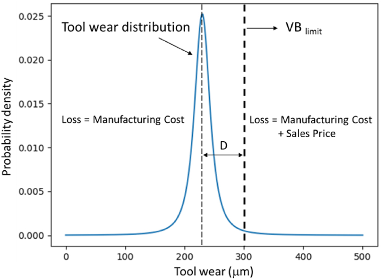
where is the sales price of one product, which includes the profit and the manufacturing cost such as the workpiece, tooling, and operating costs. The tool flank wear is denoted as , and is the limit. The term represents the probability of overused tools after the operation, which is illustrated in Fig. 1. Although most of the tool wear is under the set limit, it is always possible to exceed the set limit and cause severe damage. Balancing machining efficiency with the percentage of overusing cutting tools is the key challenge in this study.
Fig. 1.
Tool wear distribution and the loss of overusing cutting tool.
Including the loss from tool overuse, as shown in Eq. (3), into the machining process cost described in Eq. (1), the objective function that combines machining cost and the potential loss due to tool overuse is proposed as follows:
| (4) |
where is the objective function, and is a vector of variables. The symbol represents number of parts to be machined by one insert and must be an integer. The sales loss is divided by the number of parts because the objective function represents the cost per part. This loss is assumed to be shared by the parts machined with the same insert. The machining parameters are the design variables in this study, where is the cutting speed, is the feed rate, and is the depth of cut. The machining time and the tool flank wear are dependent on these three cutting parameters. However, their relationships are highly nonlinear, and no analytical expressions exist to account for the machining of varying part geometries.
The objective function is minimized using optimization techniques. Although modern optimization methods such as particle swarm optimization and genetic algorithms have proven their advantages over gradient descent, they require significantly more datasets for the optimization procedure. The absence of an analytical equation for tool wear and its variation with changing part geometries makes it difficult to generate the values of particles or genes. Furthermore, tool overuse results in failed cutting and an unevaluable objective function. This is why the gradient descent method was used in this study to gradually approach the optimal solution. The optimization process was carried out experimentally to determine the optimal turning parameters based on the objective function. The simplified conjugate gradient method was employed to solve the optimization problem [3,32]. The initial cutting parameters were defined based on the cutting tool catalog, and the parameters were normalized with respect to their initial values during the optimization process.
2.2. Termination criteria
Three termination criteria were defined to stop the iteration process in this study. The first criterion is the difference in the values of the objective function between two consecutive iterations.
| (5) |
where represents the kth iteration, and is the criterion value defined by the users. The other two termination conditions are as follows:
| (6) |
| (7) |
where is the finite difference interval of the variable for gradient calculation, is the step size along the search direction, and and are the criteria of the finite difference interval and the step size, respectively, used to stop the iteration. For a detailed explanation of the simplified conjugate gradient method used for cutting parameter optimization, refer to Ref. [3]. In the optimization procedure, the cutting parameters are expected to be increased to reduce machining time and, consequently, machining costs. However, extreme cutting parameters can result in failed operations, such as machine overloading or vibration, making it impossible to complete operations in the infeasible region. The step size or finite difference interval should be reduced to ensure that the optimization process remains within the feasible region and converges properly.
Nevertheless, tool wear variations may introduce uncertainty into the experimental data. If the finite difference interval and step size are too small, the optimization procedure can become unstable and may not reach completion. Therefore, appropriate criteria for the finite difference interval and step size are necessary to terminate the process effectively.
2.3. Determination of sample size
Taylor's equation or its extensions have been used in many studies on machining economics. These equations are deterministic, estimating tool wear based on cutting parameters. However, tool wear is probabilistic, even under the same cutting parameters. If the optimum parameters are obtained using deterministic equations without considering the distribution of tool wear, the cutting tool could reach the end of its life before completing the operation. This would lead to rework or the scrapping of failed parts, causing significant losses for manufacturers.
A probability density function of tool wear is necessary for robust optimization, and its accuracy depends on the sample size. However, performing many operations with the same cutting parameters can make the optimization process tedious and inefficient. To determine the appropriate sample size, this study adopts the concept of the confidence interval (CI). A one-sided CI with an upper bound is used as follows [34]:
| (8) |
where is the sample mean of tool flank wear, is the right-tailed critical value of the confidence interval at a level based on the t-distribution, is the sample standard deviation, and represents the sample size. When the sample mean is obtained, the question arises how close the sample mean is to the true mean. The confidence interval defines the range within which the true mean lies, given a certain confidence level. A smaller confidence interval indicates higher accuracy of the sample mean. The confidence interval can also be interpreted as an estimated error when using the sample mean. If a series of tests is conducted, the sample mean, standard deviation, and confidence interval can be calculated.
In this study, the sample size is determined by the confidence interval. If the confidence interval indicates a low probability of exceeding the tool wear limit, it is acceptable to continue the optimization process with the current sample size. Otherwise, the sample size must be increased to obtain a more accurate probability distribution. Increasing the sample size narrows the t-distribution until it closely approximates a normal distribution. Initially, a small number of tests may suffice if the sample mean is far from the tool wear limit. However, as the mean approaches the set limit, increasing the sample size is crucial for accurately defining the tool wear distribution. Therefore, the sample size is considered adequate if the upper bound of the confidence interval is smaller than the tool wear limit, as follows:
| (9) |
Equation (9) can be rewritten as follows.
| (10) |
where is the estimated difference between the tool wear limit and the mean. Equation (10) can be modified to determine the sample size as follows.
| (11) |
However, the estimated difference approaches zero when the mean is near the tool wear limit, resulting in a large sample size. This problem is addressed by modifying the definition of the estimated difference as follows:
| (12) |
where and are two positive constants used to adjust the estimated wear difference in the optimization procedure. The constant is applied to prevent large sample size when is close to , while is used to scale the estimated difference. Equation (11) is modified by replacing with the estimated wear difference . As shown in Equation (13), the estimated wear difference decreases as the optimization procedure approaches the set threshold of the tool wear, prompting an increase in sample size to ensure a more accurate probability distribution until the sample size becomes sufficiently large.
| (13) |
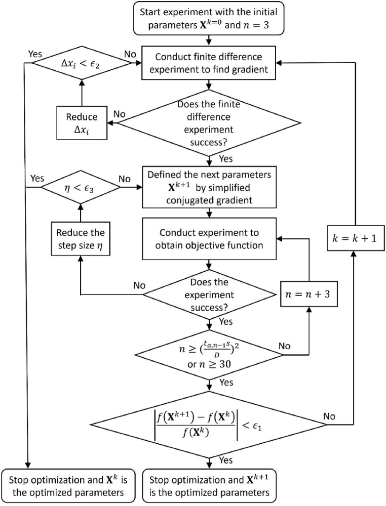
The initial sample size was set at 3. After conducting these tests, the sample mean and standard deviation were calculated, and Eq. (13) was employed to determine whether the sample size was adequate to confidently assert that the mean tool wear was sufficiently distant from the limit. If Eq. (13) was not satisfied, another 3 tests were conducted with the same cutting parameters. After every set of 3 tests, the required sample size was updated using the new sample mean and standard deviation until either Eq. (13) was satisfied or the sample size reached 30, which is assumed to be the maximum sample size for this study. The sample size would not be reduced even if calculations indicated that fewer tests were necessary in later iterations. This is due to the smaller standard deviation resulting from a larger sample size and the inherent uncertainty of experiments. Fig. 2 illustrates the flowchart of the robust optimization process for machining.
Fig. 2.
Flow chart of the robust optimization process.
3. Experimental setup
Two cases were studied to demonstrate the robust integer optimization of cutting parameters while considering tool wear distribution and discrete production. The first case involved using one cutting insert for a single part, highlighting the importance of tool wear distribution and robust optimization. The second case focused on machining multiple parts with a single cutting insert to address the challenges of discrete production. The raw material used in the experiment was a SUS 304 stainless steel bar measuring 160 mm in length and 75 mm in diameter. For both cases, the initial cutting parameters were set as follows: a cutting speed of 110 m/min, a feed rate of 0.15 mm/rev, and a depth of cut of 1.5 mm.
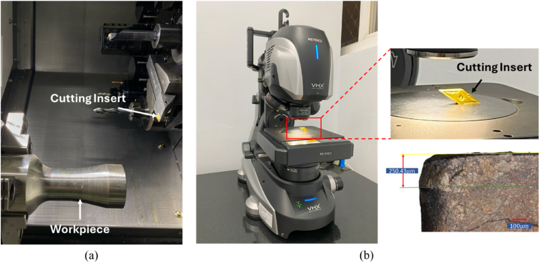
The CNC turning machine used in this study was the Force One FCL-2004, manufactured by Force One Machinery in Taiwan. This turning machine was equipped with a Siemens SINUMERIK 828D controller. Fig. 3(a) illustrates the experimental setup of the cutting tool and workpiece. The cutting tool used in the experiment was a coated carbide insert (VNMG160404-MA US735) manufactured by Mitsubishi Materials in Japan. Tool wear was monitored and analyzed using a Keyence VHX-7000 optical microscope after each turning operation, as illustrated in Fig. 3(b). The threshold for tool flank wear was set at 300 μm [35]. The design variables considered in the study included cutting speed and feed rate. Other parameters, such as depth of cut and lubrication, were excluded as they cannot be adjusted directly through the CNC controller without modifying the NC code or equipment.
Fig. 3.
(a) Experimental setup and (b) tool wear measurement.
The parameters were normalized before proceeding with the calculations for determining searching direction. The initial finite difference interval was set to be one-tenth of the initial values of the parameters, and the initial step size was set at to mitigate the influence of tool wear variation. The termination criteria , , and described in Eqs. (5), (6), (7) were established as , , and , respectively. Three tests were conducted for each parameter combination at the beginning of the optimization. The distribution of tool flank wear was incorporated into the calculation of the objective function to identify the optimum point. The constants and in Eq. (12) were set at 10 and 0.2, respectively, and the confidence level was set at 0.05.
4. Experimental results
4.1. Results of profiling one part using one cutting insert
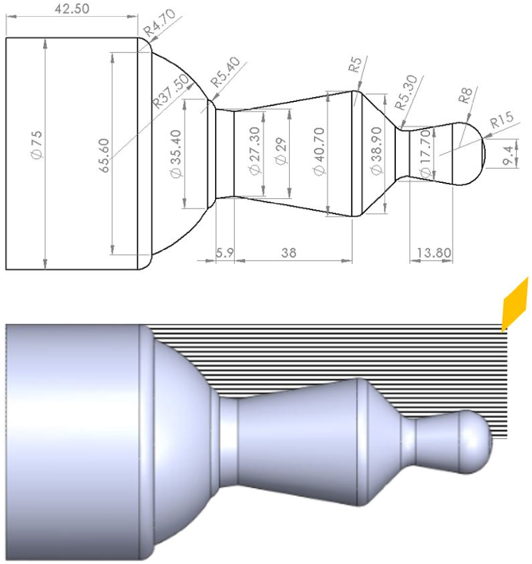
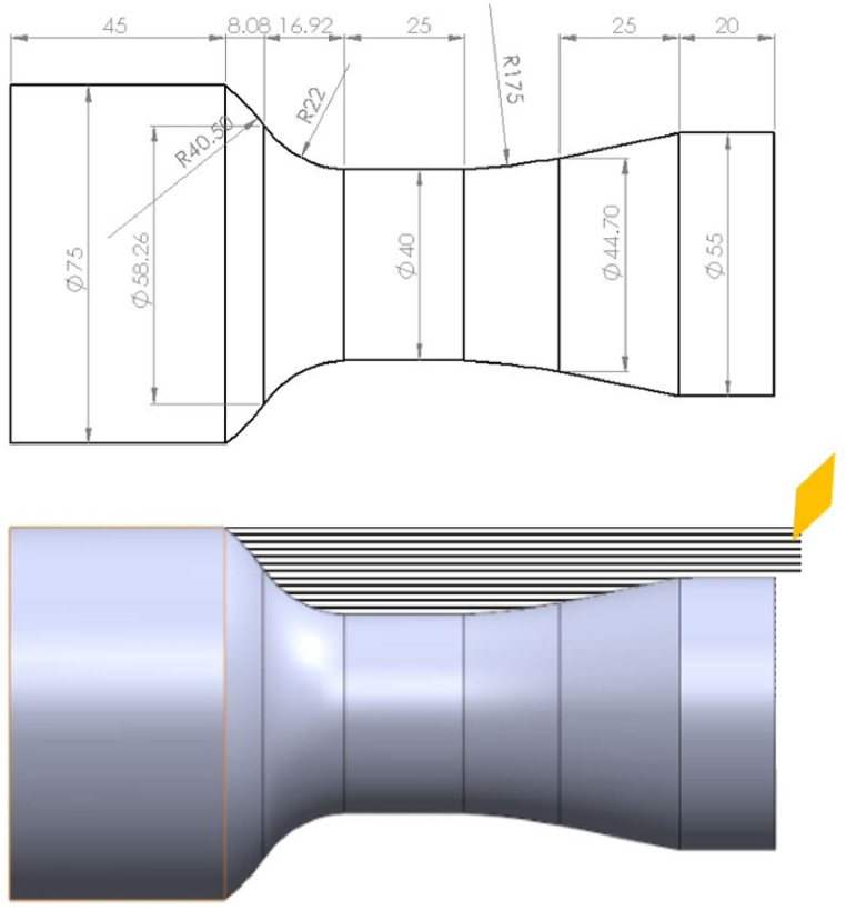
A profiling experiment was conducted under the condition that one cutting insert was used for only one part. The shape of the part is illustrated in Fig. 4, and the material removal was 328,118 mm3. The operating cost was calculated as the sum of depreciation, labor, and utility fees per unit time, assumed to be 0.2 NTD/s, 0.3 NTD/s, and 1.5 × 10⁻³ NTD/s, respectively. The costs associated with the cutting edge, workpiece, and estimated operating expense were 80 NTD, 600 NTD, and 466 NTD, respectively. It is important to note that each insert had two cutting edges available for operations. These fees were assumed based on standards in Taiwan at the time of the study and may vary depending on time and location. The profit from manufacturing one part was assumed to be 10 % of the total manufacturing cost, resulting in a sales price of 1261 NTD. In this case, it was assumed that one cutting tool was used for only one operation, and equaled 1. Additionally, and the variables , , , , and in Eqs. (2), (4) were constants, as they would not contribute to the optimization process. Consequently, the objective function was simplified as follows:
| (14) |
Fig. 4.
Part geometry and cutting paths for the first case study.
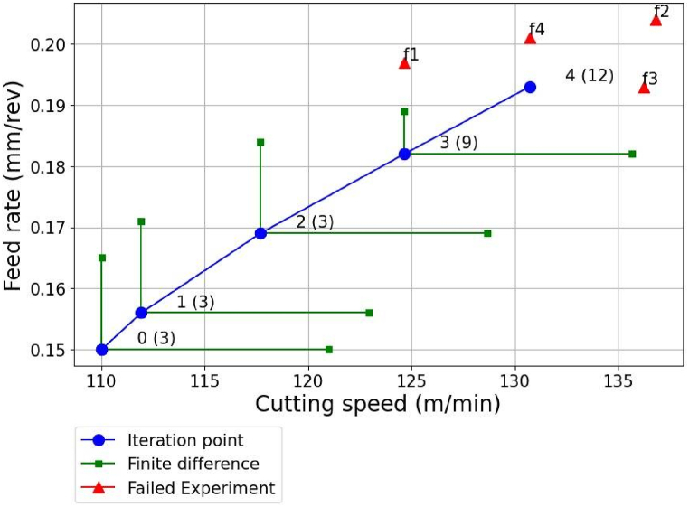
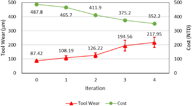
The results of the optimized cutting parameters, costs, and tool flank wear for the profiling process are presented in Fig. 5, Fig. 6. The procedure gradually converged with each iteration. After optimization, the objective function was reduced from 487.78 NTD to 352.17 NTD, while the final average tool flank wear was 217.95 μm, with a standard deviation of 35.92 μm. The optimal parameters were a cutting speed of 130.73 m/min and a feed rate of 0.193 mm/rev. A total of 12 tests were conducted in the final iteration, and the probability of tool overuse was 2 %.
Fig. 5.
Progress of cutting parameter optimization in the first case study.
Fig. 6.
Results of cost and tool wear in each iteration of the first case study.
Fig. 5 illustrates the changes in cutting parameters for each iteration, with the numbers in parentheses representing the sample sizes. From the first to the second iteration, the preset finite difference interval and step size were utilized to compute the gradient and determine the search direction. However, during the fourth iteration, the gradient calculation for the feed rate failed. To resolve this issue, both the finite difference interval and step size were reduced, allowing the completion of the fourth iteration. Nevertheless, the fifth iteration could not be completed, as the criterion for the finite difference interval in Eq. (6) was reached. Consequently, the optimization was terminated, and the optimized results were obtained in the fourth iteration.
The sample size increased throughout the optimization procedure due to the higher standard deviation and the tool wear value approaching its limit, as indicated by Eq. (13). Initially, the tool wear distribution showed a significantly lower probability of overused cutting tools, allowing the sample size to remain at 3. However, the number of tests increased to 9 in the third iteration and 12 in the fourth iteration to satisfy Eq. (13). As the average tool wear approached the set threshold, the tolerable uncertainty decreased, necessitating an increase in the required sample size to ensure it was large enough. Consequently, the sample size was expanded to validate the optimized cutting parameters as the optimization procedure neared its optimum point. The objective function was reduced by more than 27 % compared to the initial cutting parameters. It is noteworthy that while the percentage of overused cutting tools increased during the optimization, the objective function continued to decrease. This is attributed to the fact that the reduction in cutting time costs outweighed the costs associated with overused tools. The risk of producing failed parts was deemed tolerable given the low probability of overused tools in this turning operation. If the sales price were significantly higher, the optimum cutting parameters would decrease to ensure a higher yield rate.
4.2. Results of profiling multiple parts using one cutting insert
A part, as illustrated in Fig. 7, was designed for the discrete production experiment. The material removal for one workpiece was 295,288 mm3. Initially, 3 parts were machined with one insert to determine the optimized parameters for , and the initial sample size was set to 3. Therefore, a total of 9 parts needed to be machined to obtain the results in one iteration. Once the optimum solution was achieved, the number of parts was increased until the lowest cost function was confirmed. The integer optimization was conducted for the number of parts, with , and the best solution was found when . Unlike the first case, the cutting tool cost, , presetting time, , and tool replacement time, , could not be ignored in Eq. (2). The cutting tool replacement time and presetting time were assumed to be 60 and 360 s, respectively. The depreciation cost, labor cost, and utility fee per unit of time were estimated at 0.2 NTD/s, 0.3 NTD/s, and 1.5✕10−3 NTD/s. The costs for the cutting edge, workpiece, and estimated operating costs were 84 NTD, 882 NTD, and 466 NTD, respectively. The sales price was assumed to be 1389 NTD. Detailed experimental data was listed in the Appendix.
Fig. 7.
Part geometry and cutting paths for the discrete production experiment.
4.2.1. Results of profiling 3 parts
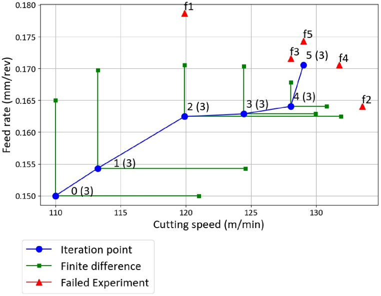
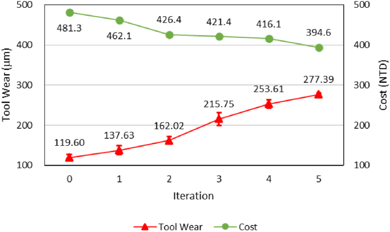
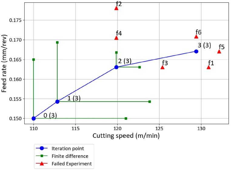
Fig. 8, Fig. 9 illustrate the optimization process and the results of the optimized cost and tool wear for profiling 3 parts. Detailed experimental data can be found in the Appendix. The red triangles in Fig. 8 represent the failed tests caused by vibrations or collapsed cutting tool edges, leading to a reduction in the finite difference interval or step size. The initial cutting parameters were a cutting speed of 110 m/min and a feed rate of 0.15 mm/rev, resulting in a cost of 481.3 NTD according to objective function Eq. (4). The cost gradually converged, and the optimization successfully reduced the objective function to 394.6 NTD with the optimal parameters of a cutting speed of 129.027 m/min and a feed rate of 0.171 mm/rev. The average tool flank wear in the optimum iteration was 277.39 μm, which is very close to the threshold of 300 μm. The standard deviation of the tool wear was 3.56 μm, and only 1.2 % of the cutting tool wear was expected to exceed the set threshold. The experiment was terminated due to the second criteria, .
Fig. 8.
Progress of cutting parameter optimization for case .
Fig. 9.
Results of cost and tool flank wear in each iteration for case .
From the first to the second iteration, the preset finite difference interval and step size were used to calculate the search direction. In the third iteration, a test with an increment in the feed rate, labeled as f1 in Fig. 8, failed due to the tool edge collapsing. To address this issue, the finite difference interval was reduced from 0.1 to 0.05 to continue the tests. Consequently, the increase in the cutting parameter for the feed rate in the third iteration was minimal. In the fifth iteration, the average tool wear reached 277.39 μm, prompting a further reduction of the finite difference interval to 0.025 after the 0.05 value failed to yield successful results. This indicates that large finite difference intervals and step sizes can lead to infeasible ranges when iterations approach the wear limit and the optimized solution. The result in the sixth iteration with a finite difference of 0.025 also failed, leading to the termination of the experiment due to the criterion being met. The objective function was reduced by 18.0 % compared to the initial cutting parameters.
4.2.2. Results of profiling 4 parts
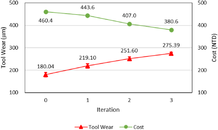
Another experiment was conducted using one insert to cut four workpieces. The results, including the progress of the cutting parameters, optimized cost, and tool flank wear, are shown in Fig. 10, Fig. 11. As in the previous experiment, the initial cutting parameters were a cutting speed of 110 m/min and a feed rate of 0.15 mm/rev, resulting in an initial cost of 460.4 NTD. This cost was lower than that for three workpieces due to the shared expenses of the cutting tool and tool replacement time. The optimization procedure gradually converged with each iteration, ultimately reducing the objective function from 460.4 NTD to 380.6 NTD. The average tool flank wear recorded was 275.39 μm, with a standard deviation of 5.29 μm. The optimum parameters identified were a cutting speed of 129.394 m/min and a feed rate of 0.167 mm/rev, with a 2.1 % probability of tool overuse. Compared to the optimized parameters in the case of , a slightly lower feed rate allowed for the extension of tool life for one additional part while further reducing manufacturing costs.
Fig. 10.
Progress of cutting parameter optimization for case .
Fig. 11.
Results of cost and tool flank wear in each iteration for case .
Fig. 10 illustrates the changes in cutting parameters across each iteration. In the first two iterations, a preset finite difference interval of 0.1 and a step size of 0.00001 were used to calculate the gradient and search direction. However, in the third iteration, the gradient calculation failed for both the cutting speed and feed rate. To complete the iteration, the finite difference was reduced to 0.05, but it failed again. Ultimately, the third iteration was successfully completed by further reducing the finite difference to 0.025. Despite this progress, the fourth iteration could not be completed, reaching the criterion for the finite difference interval. Consequently, the optimization was terminated, yielding an optimized result from the third iteration, with the objective function reduced by 17.3 % compared to the initial cutting parameters.
4.2.3. Results of profiling 5 parts
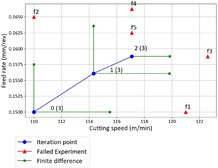
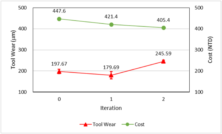
Fig. 12, Fig. 13 illustrate the optimization procedure and the results of profiling five parts using a single cutting insert. Following the optimization, the objective function was reduced from 447.6 NTD to 405.4 NTD. The optimized average tool flank wear was measured at 245.59 μm, with a standard deviation of 9.31 μm. The optimal cutting parameters were determined to be a cutting speed of 117.083 m/min and a feed rate of 0.159 mm/rev. The probability of the tool being overused was found to be 0.5 %.
Fig. 12.
Progress of cutting parameter optimization for case .
Fig. 13.
Results of cost and tool flank wear in each iteration for case .
Fig. 12 illustrates the change in cutting parameters across each iteration. In the transition from the initial to the first iteration, a preset finite difference interval of 0.1 and a step size of 0.00001 were used to calculate the gradient and search direction. However, the finite difference tests in the first iteration were unsuccessful due to overused cutting tools, labeled as f1 and f2 in Fig. 12. The recorded average tool wears were 298.42 μm and 301.76 μm, significantly higher than those observed with the initial parameters. This resulted in a higher objective function value and an inverted gradient, altering the search direction of the optimization process and hindering improvement. Consequently, these tests were deemed failures, prompting a reduction of the finite difference to 0.05 to complete the first iteration. However, the third iteration failed during the feed rate test, despite the finite difference being further reduced to 0.025. The criterion for the finite difference interval was ultimately reached, leading to the termination of the optimization process. The optimized result was obtained in the second iteration, yielding an objective function value of 405.4 NTD, representing a 9.4 % reduction compared to the initial cutting parameters.
It is evident that the insert cannot sustain high cutting efficiency when machining 5 parts, unlike when machining 4 parts. Consequently, the best solution and the lowest objective function were achieved when , with a cutting speed of 129.394 m/min and a feed rate of 0.167 mm/rev. Although the recommended cutting parameters from the catalog were lower than those obtained in this experiment, the results of this study suggest increasing these parameters to enhance cutting efficiency while ensuring the cutting tool remains sustainable.
4.3. Discussion
Cutting tool wear is not a fixed value. As demonstrated in this study, standard deviations can exceed 10 % of the mean values. Relying solely on average values in the optimization procedure poses a significant risk of overusing the cutting tool. To address this issue, this study introduced robust optimization. By incorporating the distribution of tool wear into the proposed objective function, we aimed to balance machining costs and the risk of overusing cutting tools. The results indicate that the probability of tool overusage with the optimal parameters was consistently less than 2.1 % across all cases. The losses incurred from overused cutting tools are substantially higher than machining costs, prompting the optimization process to maintain tool wear below the established limits, thereby preventing a significant increase in the objective function due to high overusage probability. Since the sales price encompasses the manufacturing cost, losses from failed products always outweigh machining costs. Consequently, it is crucial to control tool wear below the set limit. However, the decision regarding the tool wear limit ultimately depends on product quality and the load on the machine tools. In roughing operations, a higher tool wear limit may be acceptable if the resulting quality is sufficient for subsequent processes, potentially leading to further cost reductions.
Previous studies often relied on average tool wear values, treating both underuse and overuse of cutting tools with equal penalties. The ideal scenario using this approach occurs when average tool wear equals the tool wear limit [3], implying that approximately 50 % of the cutting tools would be overused. However, the costs associated with reworking or discarding defective parts far exceed those of underusing cutting tools. This discrepancy explains why most cutting tools tend to be underused [4], even though increasing cutting parameters could potentially lower costs.
In discrete production, the number of workpieces significantly impacts production costs. With the initial cutting parameters, it is expected that tool wear increases with the number of parts machined, leading to reduced costs, as shown in Table 1. However, the most economical solution after optimization was determined to be machining 4 parts. Compared to 3 parts, only a slight reduction in feed rate was necessary to ensure the cutting tool could sustain machining for 4 parts. In contrast, optimizing conditions for 5 parts required lower cutting speeds and feed rates, which substantially reduced machining efficiency and increased costs. Therefore, the optimal strategy was to cut 4 parts using a single insert. Processing a larger number of workpieces with one cutting tool does not necessarily result in lower production costs, as the reduced speeds and feed rates required for extended tool life can lead to decreased machining efficiency and potentially higher overall costs.
Table 1.
Comparison of optimization results of discrete production.
| Before Optimization | N = 3 | N = 4 | N = 5 |
|---|---|---|---|
| Cutting speed | 110 m/min | 110 m/min | 110 m/min |
| Feed rate | 0.15 mm/rev | 0.15 mm/rev | 0.15 mm/rev |
| Average tool wear | 119.60 | 180.04 | 197.67 |
| Tool wear deviation | 7.43 | 10.32 | 11.10 |
| Objective function | 481.3 NTD | 460.4 NTD | 447.6 NTD |
| After Optimization | N=3 | N=4 | N=5 |
| Optimum cutting speed | 129.027 m/min | 129.394 m/min | 117.083 m/min |
| Optimum feed rate | 0.171 mm/rev | 0.167 mm/rev | 0.159 mm/rev |
| Average tool wear | 275.39 | 245.59 | |
| Tool wear deviation | 5.29 | 5.87 | |
| Objective function | 394.5 NTD | 380.6 NTD | 405.4 NTD |
Many earlier studies utilized extended Taylor's tool life equation in their optimization efforts [11,29,31], leading to the expectation that optimized cutting parameters must be reduced to prevent tool overuse. Additionally, tool wear variations fluctuate with cutting conditions and part geometry, and there is currently no established model that accounts for these variations alongside part geometry, cutting parameters, and materials. The experimental results demonstrated a progressive improvement in machining costs while effectively limiting the overuse of cutting tools. Given the absence of an accurate model for tool wear variation in complex part geometries, the statistical analysis and experimental optimization methods proposed in this study offer a more practical approach for industrial applications.
The selection of initial cutting parameters could pose a challenge for the proposed method, potentially prolonging the optimization process. While deterministic tool wear equations may yield suboptimal solutions through numerical calculations, further verification and fine-tuning with the proposed experimental optimization method will be essential.
5. Conclusions
Robust optimization was effectively applied to the machining economics of discrete turning operations in this study. By utilizing the proposed objective function, the tool wear distribution was incorporated to manage the risk of overusing cutting tools during the optimization process. The results demonstrated that the variation in tool wear values could be accurately represented using statistical methods and included in the objective function. Only machining time and tool wear values needed to be collected after each operation for the gradient descent method. Importantly, no additional experiments were necessary to establish the coefficients of the tool wear equation, making this approach easily implementable in machine workshops to fine-tune cutting parameters.
Experiments were conducted to optimize cutting parameters across different scenarios involving the use of one cutting tool for multiple workpieces. The objective function incorporated the distribution of tool wear to balance machining costs with the risk of overusing cutting tools. Results indicated that the probability of tool overuse with the optimized parameters was less than 2.1 %, alongside reductions in objective functions ranging from 9.4 % to 27 % across the case studies. The cost associated with reworking or abandoning defective parts was significantly higher than that of underusing cutting tools. Given the lack of an accurate tool wear variation model for intricate geometries, the statistical analysis employed in this study proved practical for optimizing cutting parameters, effectively approaching optimal solutions while limiting tool overuse.
Additionally, the study highlighted that the number of workpieces processed with a single cutting tool significantly impacts production costs. Processing many workpieces with one tool does not always lead to lower costs due to reduced efficiency. In the discrete production experiment, the optimal number of parts to be cut was determined to be four, resulting in an objective function value of 380.6 NTD, lower than 394.5 NTD for cutting three parts and 405.4 NTD for cutting five parts. The acceptable tool wear limit depends on product quality and the load on the machine tools. In roughing operations, a higher tool wear limit may be acceptable if the quality remains sufficient for subsequent processes, allowing for potential cost reductions.
The optimal conditions for machining depend on specific material and part geometry. Given the variations in tool wear and complexities of part geometries, the experimental optimization method proposed in this study is particularly well-suited for industrial applications. However, numerous experiments are necessary to establish the tool wear distribution under different cutting conditions, and the development of a model for tool wear distribution would significantly enhance this research. Moreover, with increasing industry focus on energy consumption and carbon emissions, a key challenge lies in reducing energy use and emissions while maintaining production quality and efficiency.
CRediT authorship contribution statement
Chunhui Chung: Writing – review & editing, Supervision, Methodology, Funding acquisition, Conceptualization. Agus Andrianto: Writing – original draft, Investigation, Formal analysis. Po-Chieh Wang: Investigation, Formal analysis.
Data availability statement
Data included in article/supplementary material is referenced in the article.
Declaration of generative AI and AI-assisted technologies in the writing process
During the preparation of this work the authors used ChatGPT 4o in order to improve the readability and language. After using this tool/service, the authors reviewed and edited the content as needed and take full responsibility for the content of the published article.
Declaration of competing interest
The authors declare that they have no known competing financial interests or personal relationships that could have appeared to influence the work reported in this paper.
Acknowledgement
This study is supported by the National Science and Technology Council, Taiwan (Grant no. MOST 110-2221-E-006-168-MY3).
APPENDIX.
Table A.
Parameters and tool wear values in each iteration of the optimization procedure of discrete production in Section 4.2.
| Parameters with Finite Difference Interval |
Solutions in the Iteration |
|||||
|---|---|---|---|---|---|---|
| Cutting Speed (m/min) | Feed Rate (mm/rev) | Tool Wear Avg. ± Std |
Cutting Speed (m/min) | Feed Rate (mm/rev) | Tool Wear Avg. ± Std |
|
| 3 workpieces (N = 3) | ||||||
| Initial Iteration |
110.00 | 0.150 | 119.60 ± 7.43 | |||
| 1st Iteration | 121.00 | 0.150 | 141.72 ± 21.04 | 113.25 | 0.154 | 137.63 ± 11.15 |
| 110.00 | 0.165 | 152.23 ± 19.09 | ||||
| 2nd Iteration | 124.57 | 0.154 | 210.58 ± 8.20 | 119.90 | 0.162 | 162.02 ± 9.21 |
| 113.25 | 0.170 | 195.59 ± 16.95 | ||||
| 3rd Iteration | 131.89 | 0.162 | 227.14 ± 8.51 | 124.45 | 0.163 | 215.75 ± 15.80 |
| 119.90 | 0.171 | 271.73 ± 8.21 | ||||
| 4th Iteration | 129.95 | 0.163 | 260.20 ± 8.97 | 128.05 | 0.164 | 253.61 ± 10.69 |
| 124.45 | 0.170 | 255.36 ± 10.52 | ||||
| 5th Iteration | 130.80 | 0.164 | 273.06 ± 8.61 | 129.03 | 0.171 | 277.39 ± 3.57 |
| 128.05 | 0.168 | 267.05 ± 8.16 | ||||
| 4 workpieces (N = 4) | ||||||
| Initial Iteration |
110.00 | 0.150 | 180.04 ± 10.32 | |||
| 1st Iteration | 121.00 | 0.150 | 256.82 ± 9.53 | 112.83 | 0.154 | 219.10 ± 10.21 |
| 110.00 | 0.165 | 217.10 ± 14.04 | ||||
| 2nd Iteration | 123.83 | 0.154 | 242.64 ± 4.20 | 119.88 | 0.163 | 251.60 ± 8.06 |
| 112.83 | 0.169 | 239.91 ± 12.91 | ||||
| 3rd Iteration | 122.63 | 0.163 | 263.82 ± 2.97 | 129.39 | 0.167 | 275.39 ± 5.29 |
| 119.88 | 0.167 | 258.44 ± 10.79 | ||||
| 5 workpieces (N = 5) | ||||||
| Initial Iteration |
110.00 | 0.150 | 197.67 ± 11.10 | |||
| 1st Iteration | 115.50 | 0.150 | 205.25 ± 5.05 | 114.31 | 0.156 | 179.69 ± 17.17 |
| 110.00 | 0.158 | 215.53 ± 3.76 | ||||
| 2nd Iteration | 119.81 | 0.156 | 256.49 ± 10.82 | 117.08 | 0.159 | 245.59 ± 5.87 |
| 114.31 | 0.164 | 269.39 ± 9.26 | ||||
References
- 1.Taylor F.W. The American Society of Mechanical Engineers; New York: 1907. On the Art of Cutting Metals. [Google Scholar]
- 2.Panda A., Sahoo A.K., Kumar R., Das D. A concise review of uncertainty analysis in metal machining. Mater. Today-Proc. 2020;26:1734–1739. doi: 10.1016/j.matpr.2020.02.365. [DOI] [Google Scholar]
- 3.Chung C., Wang P.-C., Chinomona B. Optimization of turning parameters based on tool wear and machining cost for various parts. Int. J. Adv. Manuf. Technol. 2022;120:5163–5174. doi: 10.1007/s00170-022-09037-y. [DOI] [Google Scholar]
- 4.Sun H., Liu Y., Pan J., Zhang J., Li W. Enhancing cutting tool sustainability based on remaining useful life prediction. J. Clean. Prod. 2020;244 doi: 10.1016/j.jclepro.2019.118794. [DOI] [Google Scholar]
- 5.Mahapatra S., Das A., Jena P.C., Das S.R. Turning of hardened AISI H13 steel with recently developed S3P-AlTiSiN coated carbide tool using MWCNT mixed nanofluid under minimum quantity lubrication. Proc. Inst. Mech. Eng. Part C: J. Mech. Eng. Sci. 2023;237:843–864. doi: 10.1177/09544062221126357. [DOI] [Google Scholar]
- 6.Pradhan S., Das S.R., Jena P.C., Dhupal D. Investigations on surface integrity in hard turning of functionally graded specimen under nano fluid assisted minimum quantity lubrication. Adv. Mater. Process. Technol. 2021;8:1714–1729. doi: 10.1080/2374068X.2021.1948706. [DOI] [Google Scholar]
- 7.Hassanpour H., Rasti A., Khosrowshahi J.H., Farshi S.S. Effect of ball nose flank wear on surface integrity in high-speed hard milling of AISI 4340 steel using MQL. Heliyon. 2024;10 doi: 10.1016/j.heliyon.2024.e37337. [DOI] [PMC free article] [PubMed] [Google Scholar]
- 8.Ukamanal M., Mishra P., Sahoo A.K. Effects of spray cooling process parameters on machining performance AISI 316 steel: a novel experimental technique. Exp. Tech. 2020;44:19–36. doi: 10.1007/s40799-019-00334-y. [DOI] [Google Scholar]
- 9.Kumar R., Sahoo A.K., Mishra P.C., Das R.K. An investigation to study the wear characteristics and comparative performance of cutting inserts during hard turning. Int. J. Mach. Machin. Mater. 2018;20:320–344. doi: 10.1504/IJMMM.2018.094730. [DOI] [Google Scholar]
- 10.Panda A., Sahoo A.K., Rout A.K., Kumar R., Das R.K. Investigation of flank wear in hard turning of AISI 52100 Grade steel using multilayer coated carbide and mixed ceramic inserts. Procedia Manuf. 2018;20:365–371. doi: 10.1016/j.promfg.2018.02.053. [DOI] [Google Scholar]
- 11.Cakir M., Gurarda A. Optimization and graphical representation of machining conditions in multi-pass turning operations. Comput. Integr. Manuf. Syst. 1998;11:157–170. doi: 10.1016/S0951-5240(98)00015-9. [DOI] [Google Scholar]
- 12.Lee B.Y., Tarng Y.S. Cutting-parameter selection for maximizing production rate or minimizing production cost in multistage turning operations. J. Mater. Process. Technol. 2000;105:61–66. doi: 10.1016/S0924-0136(00)00582-3. [DOI] [Google Scholar]
- 13.Hippalgaonkar R., Shin Y. Robust optimisation of machining conditions with tool life and surface roughness uncertainties. Int. J. Prod. Res. 2011;49:3963–3978. doi: 10.1080/00207543.2010.495207. [DOI] [Google Scholar]
- 14.Das D., Thakur R.K., Chaubey A.K., Sahoo A.K. Optimization of machining parameters and development of surface roughness models during turning Al-based metal matrix composite. Mater. Today-Proc. 2018;5:4431–4437. doi: 10.1016/j.matpr.2017.12.011. [DOI] [Google Scholar]
- 15.Jena J., Panda A., Behera A.K., Jena P.C., Das S.R., Dhupal D. In: Innovation in Materials Science and Engineering. Chattopadhyay J., Singh R., Prakash O., editors. Springer; Singapore: 2019. Modeling and optimization of surface roughness in hard turning of AISI 4340 steel with coated ceramic tool; pp. 211–216. [Google Scholar]
- 16.Xu L., Huang C., Li C., Wang J., Liu H., Wang X. Estimation of tool wear and optimization of cutting parameters based on novel ANFIS-PSO method toward intelligent machining. J. Intell. Manuf. 2021;32:77–90. doi: 10.1007/s10845-020-01559-0. [DOI] [Google Scholar]
- 17.Kumar P., Misra J.P. Process modeling and optimization using ANN and RSM during dry turning of titanium alloy in automotive industry. Proc. Inst. Mech. Eng. - Part D J. Automob. Eng. 2020;235:2040–2050. doi: 10.1177/0954407020969255. [DOI] [Google Scholar]
- 18.Bagaber S.A., Yusoff A.R. Energy and cost integration for multi-objective optimisation in a sustainable turning process. Measurement. 2019;136:795–810. doi: 10.1016/j.measurement.2018.12.096. [DOI] [Google Scholar]
- 19.Rajemi M.F., Mativenga P.T., Aramcharoen A. Sustainable machining: selection of optimum turning conditions based on minimum energy considerations. J. Clean. Prod. 2010;18:1059–1065. doi: 10.1016/j.jclepro.2010.01.025. [DOI] [Google Scholar]
- 20.He K., Tang R., Jin M. Pareto fronts of machining parameters for trade-off among energy consumption, cutting force and processing time. Int. J. Prod. Econ. 2017;185:113–127. doi: 10.1016/j.ijpe.2016.12.012. [DOI] [Google Scholar]
- 21.Zhang Z., Wu L., Jia S., Peng T. Multi-objective parameter optimization to support energy-efficient peck deep-hole drilling processes with twist drills. Int. J. Adv. Manuf. Technol. 2020;106:4913–4932. doi: 10.1007/s00170-020-04967-x. [DOI] [Google Scholar]
- 22.Li C., Wu S., Yi Q., Zhao X., Cui L. A cutting parameter energy-saving optimization method considering tool wear for multi-feature parts batch processing. Int. J. Adv. Manuf. Technol. 2022;121:4941–4960. doi: 10.1007/s00170-022-09557-7. [DOI] [Google Scholar]
- 23.Jia S., Wang S., Zhang N., Cai W., Liu Y., Hao J., Zhang Z., Yang Y., Sui Y. Multi-objective parameter optimization of CNC plane milling for sustainable manufacturing. Environ. Sci. Pollut. Res. 2022 doi: 10.1007/s11356-022-24908-3. [DOI] [PMC free article] [PubMed] [Google Scholar]
- 24.Cao M., Zhou C., Li K.M. Research on the relationship between workpiece surface machining quality and turning tool wear. J. Phys. Conf. Ser. 2021;2029:13–15. doi: 10.1088/1742-6596/2029/1/012071. [DOI] [Google Scholar]
- 25.Liu C., Li Y., Hua J., Lu N., Mou W. Real-time cutting tool state recognition approach based on machining features in NC machining process of complex structural part. Int. J. Adv. Manuf. Technol. 2018;97:229–241. doi: 10.1007/s00170-018-1916-y. [DOI] [Google Scholar]
- 26.Swain S., Panigrahi I., Sahoo A.K., Panda A., Kumar R. Effect of tool vibration on flank wear and surface roughness during high-speed machining of 1040 steel. J. Fail. Anal. Preven. 2020;20:976–994. doi: 10.1007/s11668-020-00905-x. [DOI] [Google Scholar]
- 27.McParland D., Baron S., O'Rourke S., Dowling D., Ahearne E., Parnell A. Prediction of tool wear in turning of medical grade cobalt chromium molybdenum alloy (ASTM F75) using nonparametric Bayesian models. J. Intell. Manuf. 2019;30:1259–1270. doi: 10.1007/s10845-017-1317-3. [DOI] [Google Scholar]
- 28.Ráczkövi L. Tool life of cutting tool in case of hard turning. Hung. J. Ind. Chem. 2010;38:133–136. doi: 10.1515/289. [DOI] [Google Scholar]
- 29.Sahoo A., Orra K., Routra B. Application of response surface methodology on investigating flank wear in machining hardened steel using PVD TiN coated mixed ceramic insert. Int. J. Ind. Eng. Comput. 2013;4:469–478. doi: 10.5267/j.ijiec.2013.07.001. [DOI] [Google Scholar]
- 30.Chua M.S., Loh H.T., Wong Y.S., Rahman M. Optimization of cutting conditions for multi-pass turning operations using sequential quadratic programming. J. Mater. Process. Technol. 1991;28:253–262. doi: 10.1016/0924-0136(91)90224-3. [DOI] [Google Scholar]
- 31.Sardiñas R.Q., Santana M.R., Brindis E.A. Genetic algorithm-based multi-objective optimization of cutting parameters in turning processes. Eng. Appl. Artif. Intell. 2006;19:127–133. doi: 10.1016/j.engappai.2005.06.007. [DOI] [Google Scholar]
- 32.Cheng C.H., Chang M.H. A simplified conjugate-gradient method for shape identification based on thermal data. Numer. Heat Transf. B: Fundam. 2003;43:489–507. doi: 10.1080/713836242. [DOI] [Google Scholar]
- 33.Stephenson D.A., Agapiou J.S. second ed. CRC Press, Taylor & Francis Group; Boca Raton: 2005. Metal Cutting Theory and Practice. [Google Scholar]
- 34.Tamhane A., Dunlop D. first ed. Prentice Hall; Upper Saddle River, NJ: 2000. Statistics and Data Analysis: from Elementary to Intermediate. [Google Scholar]
- 35.International Organization for Standardization . International Organization for Standardization; Geneva: 1993. ISO 3685:1993 Tool-Life Testing with Single-Point Turning Tools. [Google Scholar]
Associated Data
This section collects any data citations, data availability statements, or supplementary materials included in this article.
Data Availability Statement
Data included in article/supplementary material is referenced in the article.


