A reinforcement learning approach to effective forecasting of pediatric hypoglycemia in diabetes I patients using an extended de Bruijn graph

Abstract

Pediatric diabetes I is an endemic and an especially difficult disease; indeed, at this point, there does not exist a cure, but only careful management that relies on anticipating hypoglycemia. The changing physiology of children producing unique blood glucose signatures, coupled with inconsistent activities, e.g., playing, eating, napping, makes “forecasting” elusive. While work has been done for adult diabetes I, this does not successfully translate for children. In the work presented here, we adopt a reinforcement approach by leveraging the de Bruijn graph that has had success in detecting patterns in sequences of symbols–most notably, genomics and proteomics. We translate a continuous signal of blood glucose levels into an alphabet that then can be used to build a de Bruijn, with some extensions, to determine blood glucose states. The graph allows us to “tune” its efficacy by computationally ignoring edges that provide either no information or are not related to entering a hypoglycemic episode. We can then use paths in the graph to anticipate hypoglycemia in advance of about 30 minutes sufficient for a clinical setting and additionally find actionable rules that accurate and effective. All the code developed for this study can be found at: https://github.com/KurbanIntelligenceLab/dBG-Hypoglycemia-Forecast.

Introduction

While diabetes mellitus is ranked eighth in the leading causes of noncommunicable diseases¹ with significantly more than an estimated 500 million people affected worldwide^2,3, the metabolic complications that arise transform it into a systematic disease e.g., cardiovascular disease^4,5, neuropathy⁶, nephropathy⁷, retinopathy⁸, and even cancer^9,10. Exacerbating the effects of diabetes are the continual self-monitoring and self-care that studies show are generally not followed^11–13. The most pernicious aspect is hypoglycemia (See Fig. 1), also called low blood glucose, occurring as blood glucose falls below normal, healthy levels. In fact, hypoglycemia is among the major limiting factors in achieving normal glycemia, since it can unexpectedly occur with varying degrees of severity that manifests as profuse sweating, heart palpitations, confusion and disorientation, and intense hunger with more than five episodes, on average, per month¹⁴.

Fig. 1.

(Left) shows critical pathways that cause hypoglycemia–insulin cannot be decreased and glucagon cannot be increased. (Right) physiological response. The graphic exposes both the complexity and challenges in determining this state which is often defined only by plasma glucose between 55-70 mg/dl often occurring when therapeutic intervention includes meglitinides, sulfonylureas, or insulin since drugs themselves are among the most common causes. Glu (glucose), INS (insuline), EPI (epinephrine).

Understandably, patients generally develop anxiety and even fear of hypoglycemic episodes that affects both self-monitoring and self-care^15,16. Adolescent hypoglycemia episodes are the most severe^17,18 warranting improvements in technology for anticipation of spikes.

Traditionally, the glucose value mmol/L (70 mg/dl) is used as the clinical alert or threshold value for initiating treatment for hypoglycemia because of the potential for glucose to fall even further and especially to anticipate consequences of glucose levels below 3 mmol/L (54 mg/dl). Children with type 1 diabetes (T1D) should spend less than 4% of their time mmol/L (70 mg/dl) and less than 1% of their time mmol/L (54 mg/dl).

Driven by the anxiety of hypoglycemia, overtreating, even before reaching the threshold, is very common. In practice, aggravating this problem is the need to lower the threshold for hypoglycemia (60 or 65mg/dl) in order to stabilize the glycemic variations. In addition, new stable insulin formulations (rapid and shorter acting insulin as well stable and flatter long-acting insulin) contribute to fewer variations. Pairing glucose sensors and automated insulin delivery systems may also improve treatment in reducing hypoglycemic events with more precise and accurate prediction to adjust insulin dose but that can taken into account age-specific attributes¹⁹. Thus, a critical use of artificial intelligence (AI) would be to improve clinical forecasting of blood glucose (BG) levels in pediatric T1D, since children are particularly vulnerable. This group’s forecasting problems are more difficult because of the lack of routine in their days, e.g., snacks, play, rest, missed injections, misreading levels. From one perspective, this is a classification problem with two definable regions and margin between (See Fig. 2), but on the other hand it is a forecasting problem. The principle challenge for this hybrid problem (including overtreatment) is that the signal behaves erratically due to accompanying adolescent behaviors. A natural approach to address this problem is to use state-of-the-art (SotA) temporal algorithms, e.g. Time Series Library (TSlib)²⁰ located https://github.com/thuml/Time-Series-Library that procures and provides the current best implementations (the “leaderboard”) with accompanying papers contributed currently by more than two dozen researchers. We found, surprisingly, that they fail. Examining the data, we discover it is non-stationary which violates strong statistical assumptions that most of these algorithms require. In this work we take a very different, novel approach: exploit reinforcement learning to build a de Bruijn graph (dBG) (extending the definition of Markov Decision Processes) by creating an alphabet over patient temporal BG sensor readings and integrate an input window reflecting numerical intervals. And rather than using a single state context to make a prediction as has been traditionally done, we allow multiple states to contribute. We then tune, what we call the resolution (fewer or greater number of edges based on weight), to prune out the less relevant paths. As sensor data is given, our structure can effective forecast when a hypoglycemic episode within acceptable clinical accuracy.

Fig. 2.

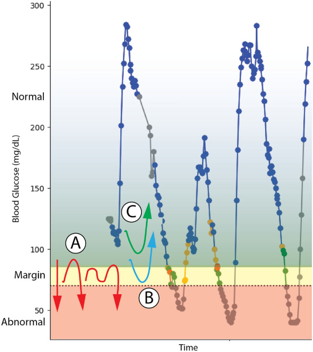
A sample time series for adolescent T1D showing BG levels. The green region is normal (safe), yellow is the margin between normal and abnormal, and red is abnormal where BG levels are life-threatening. The problem is of two types: classify, but also forecasting. (A) shows a collection of paths that lead to the abnormal region. (B, C) looks as though they will be in the abnormal, but are not.

The contributions in this work are: developing a novel, effective reinforcement learning approach to address the critical problem of pediatric T1D forecasting well-enough that a solution could exist in real clinical settings. The graph solution can forecast when a hypoglycemic episode will subsequently occur within 30 minutes with acceptable clinical accuracy. We demonstrate both the model effectiveness and run-time efficiency of building essentially a kind of state machine that can recognize subtle changes and, when run as a generator, can produce actionable patterns. Further, since this is a lazy structure, a new patient with limited data find the best set of graphs and then modify them to suit her needs. Fig. 3 (II.-IV.) highlights the process using a small data sample. We also provide a usual non-stationary test for the data as well as comparing our solution against 13 SotA implementations that show the dBG outperforms SotA solution. Further, the training time is orders of magnitude less.

Fig. 3.

(I) A dBG for 4-tuples over . Observe the Eularian path (A,B,, P) that captures all tuples. Many properties exist like reflection of graph. The de Bruijn sequence itself is lower left, A the start and P the end and is the most efficient encoding. By moving of this so-called drum, each 4-tuple can be recovered. (II) A snapshot of 15 minute intervals of a pediatric patient BG levels. We selected one that was reasonably easy to visualize, but even this one exhibits challenges in data. (III) A representation of the discretization and symbolics for II. Observe that the sharp changes in II. are still captured representing idiosyncrasies of the patient–perhaps exercise, eating, napping, signal problems. (IV) This shows a portion of our dBG representation. The path is shown (A,B,,I) given unique four-tuples with edges showing counts that characterize patterns beginning with 10.

This paper is structured as follows: Section 2 provides the background. Section 3 details our dBG. Experimental results and conclusion are presented in Sections 4 and 5, respectively.

Background and related work

Predicting both short and long-term BG concentration is crucial in diabetes management. Access to reliable algorithms for forecasting BG and hypoglycemic episodes enables proactive treatment and refined carbohydrate control, potentially preventing critical events. Despite the advancements in classification- or regression-based methods^21–23, a universally effective prediction approach remains elusive, furthering the need for exploration and innovation. Current research predominantly employs Continuous Glucose Monitoring (CGM) data along with other physiological parameters for prediction, but a limited number focus exclusively on CGM data. This gap is even more pronounced in pediatric research, where managing hypoglycemia is compounded by the unpredictability of children’s routines and hormonal changes leading to insulin resistance²⁴. Earlier studies present diverse methods for BG prediction, e.g., autoregressive moving-average models and various machine learning algorithms^25–28. While recent models employing neural networks and ensemble machine learning show promise^29–33, the complexity of pediatric diabetes is proving harder to model; some research aims at improvement by constraining time periods, e.g., nocturnal hypoglycemia prediction models and variable importance plot feature selection^34,35. The most significant work we found studied ten virtual pediatric patients³⁶ using recurrent Neural Networks (RNNs) and Long Short-Term Memory (LSTM) networks. While the results were promising, the nature of the data makes clinical evaluation difficult at best and adoption unlikely. Reinforcement learning (RL)³⁷ is now the most popular AI in ubiquitous use due to its generality across divers problems. RL is based, from one powerful perspective, on Markov decision processes that characterize a problem into searching through states sequentially with limited feedback.

In the field of time series forecasting, recent advancements have been driven by innovations in Transformer-based models, addressing challenges of long-sequence forecasting. TSLib is a comprehensive library that consolidates a range of Transformer-based models developed by various researchers, supporting diverse time series tasks such as long- and short-term forecasting, anomaly detection, and more. We chose to work with this repository to gain convenient access to numerous SotA models.

Among the notable models in TSLib, Reformer³⁸ proposes a locality-sensitive hashing algorithm to improve the attention time complexity to . The Informer³⁹ achieves a similar time complexity using their ProbSparse self-attention mechanism. Pyraformer⁴⁰ proposes a multi-resolution representation of the time series. Autoformer⁴¹ replaces the self-attention mechanism with an Auto-Correlation mechanism for long-term forecasting based on the series periodicity. FEDFormer⁴² aims to capture seasonal-trends long with other series components to make long-term forecasts. In contrast, LightTS and DLinear^43,44 propose simpler approaches, with LightTS offering a robust MLP-based architecture and DLinear demonstrating the surprising efficacy of linear models over complex Transformer-based systems. Timesnet, PatchTST, and iTransformer^45,46,20 further diversify the landscape, with Timesnet focusing on 2D tensor transformation of time series, PatchTST employing segmentation for forecasting accuracy, and iTransformer redefining the use of Transformers in forecasting with a focus on variate-centric representations. Non-stationary Transformers⁴⁷ focuses on non-stationary data as traditional methods used to improve predictability often remove critical non-stationary elements. Multi-scale Isometric Convolution Network (MICN)⁴⁸ combines local features and global correlations to capture the overall view of time series, including fluctuations and trends. Frequency improved Legendre Memory model (FiLM)⁴⁹ enhances the preservation of historical information in neural networks using Legendre Polynomials projections while minimizing overfitting to noise. In this work, since these models have not been evaluated on any data akin to adolescent T1D and are not as well-known or regarded, we chose to evaluate against both well-known and regarded algorithms that have been used in various, diverse data.

We chose to use the dBG⁵⁰ originally a structure used to efficiently encode sequences as a Eularian path. dBG have been adopted as approaches across a number of domains where the problem can be cast a sequence of events, cryptology^51,52, sequence complexity^53–55, networks⁵⁶, genomics (especially assembly)^56–62. In our recent work, we demonstrated that the dBG model is highly effective for representing univariate time series data⁶³. In particular, after construction, the dBG can characterize subtle patterns of events (or symbols) either as a recognizer or producer (much like a regular expression and its equivalent deterministic finite automaton). We imagined treating the BG levels as a sequence of events (symbols) and investigate how well a dBG can capture and detect patterns.

Methods

The research was reviewed by the Institutional Review Board (IRB) of Sidra Medicine, Doha, Qatar. It provided approval following Sidra’s Policies and Procedures about Human Research Protection. The IRB of Texas A &M University (College Station, TX, USA) uses a dual oversight review to confirm that the research satisfies the requirements of the common rule. The experimental protocol was approved by the Institutional Review Boards of Sidra Medicine (1536095) and Texas A &M University (IRB2019-0378F). All methods were performed in accordance with relevant guidelines and regulations.

Notations

For an alphabet and positive integer k,⁶⁴ describes a recursive algorithm to generate the most efficient encoding of all k sequences as a single sequence, called a de Bruijn sequence (2,k), where each substring (also known as k-tuple or k-mer) occurs only once in s modulo . For example, describes and . Fig. 3 (I) shows the de Bruijn graph for 4-tuples. This result was discovered both earlier⁶⁵ and simultaneously⁶⁶, but de Bruijn’s approach using graphs proved the most accessible. The power of this representation is that by traveling the Eularian path, every k-tuple (in this case 4) is encountered. The sequence is shown as the usual drum bottom left. The vertices are all possible sequences of length k, while the edges represent shared subsequences from the directed edge pair, the suffix and prefix, respectively. The alphabet size was soon extended to an arbitrary, but finite size. The associated graph is written is defined with vertices and edges .

We develop notation to sufficiently understand the stationarity test. Temporal models generally cast as indexed stochastic processes⁶⁷ as random variable and more completely as where t indexes the time of a multvariate process and . In our case discrete which has no significant difference in this case. The time series is really a shorthand for the join distribution . Temporal data has (strong) stationarity⁶⁸ if any finite collection of random variables is identical to any other, in symbols for any .

Data, transformation, and discretization

This research employs data from 15 pediatric diabetes patients, totaling 22,291 BG level measurements. The hypoglycemia threshold is set at 70 mg/dL. Despite the dataset’s average 15-minute sampling rate, it exhibits variations and significant gaps, ranging from a few hours to several days. To address this, gaps exceeding 20 minutes are processed as separate sequences during modeling. These gaps have numerous causes that are simply a part of any sensor of this ilk. Comprehensive patient information is tabulated in Table 1.

Table 1.

Patient information for the study.

Patient	Datapoints (% Hypo.)	Study days	Age	Gender	Weight (kg)	Height (cm)	BMI	Years with T1D
P1	1422 (63.7 %)	18	16	M	142	168	50.3	3 (T2D)
P8	1325 (7.92 %)	17	14	M	60	166	21.8	7
P9	1530 (3.53 %)	14	11	F	50	147	23.1	4
P10	1444 (10.66 %)	14	16	F	50	163	18.8	12
P11	1686 (0.95 %)	14	14	F	49	153	20.9	3
P13	826 (1.94 %)	18	13	F	40	146	18.8	2
P16	1395 (5.09 %)	14	13	M	40	150	17.8	12
P17	1642 (1.28 %)	14	11	M	50	151	21.9	3
P18	1929 (6.48 %)	19	15	F	73	153	31.2	7
P19	1318 (10.09 %)	14	16	F	56	155	23.2	7
P20	719 (7.79 %)	20	14	F	64	163	24.1	4
P21	1014 (9.27 %)	20	14	F	64	155	26.6	8
P24	2631 (5.13 %)	15	14	M	55	183	16.4	2
P26	2089 (14.60 %)	21	8	F	26	126	16.4	4
P30	1321 (0.53 %)	14	15	F	61	161	23.5	4

T2D stands for type 2 diabetes.

The dBG model requires initial data discretization, operating on an alphabet instead of the continuous space used in BG. A larger alphabet size () minimizes information loss during discretization but reduces the model’s generalizability by increasing the number of unique k-tuples. To balance this trade-off, we use a uniform discretization approach, where normoglycemia values () are represented by 10-unit ranges. This minimizes alphabet size while preserving essential dataset trends. The model assigns 12 characters for normoglycemia, two for hypoglycemia, and one for hyperglycemia, totaling 15 characters. Fewer labels are applied in the hypoglycemia and hyperglycemia ranges, where predictions are less relevant for future states, although an additional hypoglycemia label enhances resolution within this critical region. Table 2 provides the complete set of discretization labels for corresponding BG values.

Table 2.

Discretization labels and their frequency in the dataset.

Attribute	(0-60]	(60-70]	(70-80]	(80-90]	(90-100]	(100-110]	(110-120]	(120-130]	(130-140]	(140-150]	(150-160]	(160-170]	(170-180]	(180-190]	(190-500]
Label	0	1	2	3	4	5	6	7	8	9	10	11	12	13	14
Frequency	1418	872	878	1122	1471	1424	1265	1084	1035	957	1050	1005	944	826	6940

The 0 and 1 labels represent hypoglycemia values.

Algorithms for model construction

The model begins by constructing a dBG from the discretized data input, denoted as , where is a given alphabet of the sequences. In the dBG, each node represents a unique -tuple from the original sequence, and each edge signifies a sequential transition between two -tuples, forming a k-tuple. Edge weights indicate the k-tuple transition frequency within the dataset. The dBG construction algorithm can be implemented in time complexity using a sliding window. The choice of k influences the dBG’s structure. In our model, -tuples serve as the input window, utilized for future predictions. Fig. 4 (Left) illustrates a high level visualization of a graph generated with all patients.

Fig. 4.

(Left) A high-level visualization of a dBG with 97 nodes and 167 edges using all available patients. The dBG is pruned with 10 uniform weight threshold. There are three BG regions: hyperglycemic, normal, and hypoglycemic. Dark blue nodes correspond to hypoglycemic values, while red nodes denote hyperglycemic values. (White arrows) Edge thickness indicates the frequency of the k-tuples, offering visual insight into their prevalence. (Brown arrows) There are only a few paths between the three regions and interestingly, all paths must path through normal BG. These ingress/egress paths are at the kernel of rules for anticipating hypoglycemia. (Right) Evaluation of patient results using leave-one-out cross-validation. We assessed the Balanced Accuracy, Precision, Sensitivity, and Specificity for all patients employing the leave-one-out cross-validation method. The average scores across all patients were 0.844, 0.268, 0.801, and 0.887 for these metrics, respectively. Additionally, the model achieved an F1 score of 0.402 and an Area Under the Curve of 0.89. These evaluations were conducted using adaptive pruning and with the parameters .

Graph pruning

The analysis emphasizes frequent transitions, necessitating dBG pruning to exclude anomalies. Despite the simplicity of flat pruning, applying a universal threshold, as visualized in Fig. 4 (Left), may not be optimal. It disregards the varying significance of edges in predicting imminent hypoglycemia episodes. Hypoglycemia nodes () are defined as nodes containing at least one hypoglycemia value in their -tuple, represented by the symbols “0” and “1” in our alphabet. In the dBG, edges closer to any node hold greater relevance for hypoglycemia forecasting, justifying a less stringent pruning condition for these edges.

Algorithm 1.

AdaptivePruning.

Definition 1

Given a node , let represent the shortest unweighted path distance to the nearest .

Define as a list of ordered pairs, representing non-overlapping semi-open intervals where . Let with ordered values. Define the mapping function for every range in to a corresponding threshold in , . We thus define if . Edges with a weight can be now be pruned. For larger datasets, a continuous version is also viable. This thresholding method prioritizes the retention of vital edges that boosts predictive accuracy. See Algo. 1 for the adaptive pruning implementation using . For this study we used when , when and when .

Algorithm 2.

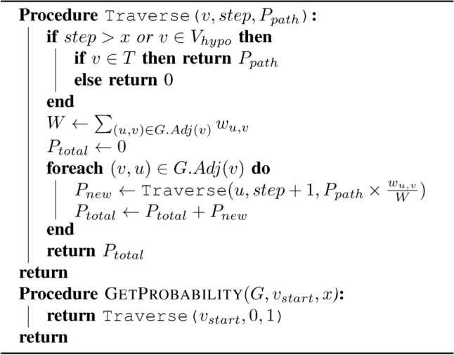
GetProbability.

Making predictions

To predict with a dBG, we use an input -tuple, aiming to decide on alert issuance at the item. This tuple is analyzed within the dBG nodes to infer the most likely subsequence trajectory. As each path sequence frequency is identifiable by edge weights, it assists in estimating the probability of reaching any node from a starting node. Our focus is on predicting a hypoglycemic episode for the patient. For each node, the likelihood of reaching a node is calculated, constrained by a parameter , denoting the search end either by steps or upon reaching a node. This probability is represented as for a node . Consider nodes v (current) and (nearest hypoglycemia node), and let denote the set of all paths shorter than x between v and . Define Let the edge (u, v) traversal probability be , and the path probability be . The overall probability is then . Alerts for tuple v are issued as follows:

1

Refer to Algo. 2 for the detailed computation of the probability for each node. With these probabilities, predictions become straightforward. We introduce a threshold parameter, , to trigger an alert for potential hypoglycemic episodes when . can be adjusted to tune alert sensitivity. If the input sequence for a prediction is absent in our graph, the algorithm employs the Euclidean distance to identify and base predictions on the nearest existing node.

Graph update

The dBG model excels in its ease of updating, eliminating the need for total graph reconstruction. This feature is particularly beneficial for large-scale applications. A graph database, constructed from prior patients exhibiting diverse BG traits, facilitates the seamless integration of new patient data. This new data aids in the pinpointing and enhancement of the most compatible model from the database, further fine-tuning its applicability to subsequent patients. The update process is efficient: new edges are added for non-existent tuples, and existing edge weights are incremented, all accomplished with an time complexity. The default weight increment is one, adjustable for more substantial graphs.

Results

In our approach for model evaluation, every normoglycemia datum is considered (no reduction). For any t, we assess the possible hypoglycemic values . Adhering to clinical best practices, we establish our goal of 30 min. forecasting window. Let h be the start of the closest hypoglycemia instance in the future. If and an alert is issued at instance t, then it’s deemed a correct prediction. Our evaluation leveraged a leave-one-out cross-validation, with each patient’s data processed separately.

Model supervision

Our preliminary demonstration of the model on patient P21 is depicted in the upper timeline of Fig. 5. The model adeptly predicts hypoglycemic events prior to their occurrence, signified by green markers. Nonetheless, a significant limitation is the consistent generation of false alerts, denoted by yellow markers, post-return to normoglycemia from a hypoglycemic state. To mitigate these false predictions, our model is enhanced with an additional supervisory system. This auxiliary system employs a fundamental rule set , designed to annul the initial prediction under specific conditions. Let S be the raw (un-discretized) test sequence and i be the index of the datapoint that we are predicting within S. Then where . Observe that alerts will be suppressed if , or BG ascends by more than 15 mg/dL from the preceding reading.

Fig. 5.

Timelines of alert predictions for P21. Correct and wrong predictions are marked with different colors. Gray data points are not used for evaluation, possibly due to the patient already being in a hypoglycemic state or gaps in the timeline. The upper timeline uses our dBG model, while the lower timeline uses the supervision ruleset along with the dBG model. Parameters: .

The enhanced model, inclusive of supervisory intervention, is showcased in the lower timeline for patient P21 in Fig. 5. Despite the efficacy of this rule set for the majority, it retains adaptable for tailoring to individual patient requirements for superior results. Stricter rule application may elevate the count of False Negatives while curtailing False Positives, necessitating a judicious balance to ensure an optimal trade-off.

Evaluation results

First established in econometrics, the Kwiatkowski-Phillips-Schmidt-Shin (KPSS) test⁶⁹ is used for testing whether times series data is stationary around a deterministic trend and is more sensitive than the alternative of a unit root. While not perfect (no single test exists), KPSS does do well in practice since root tests suffer from both size and low power⁷⁰. Since SotA use stationarity (as all temporal analysis does), we examined our time series data to establish some initial understanding of why all the SotA implementations performed so much worse and in many cases badly. Table  3 provides a consist lack of stationarity in all the adolescent BG levels. The results show that the test statistic is greater than the critical value (CV) and the p-value allows rejection of alpha level in virtually all patients. The principle weakness of KPSS is that Type I errors are more common, but increasing p-values affects the power.

Table 4.

(A) Model performance using different parameters.

Comprehensive Model Evaluation Metrics
Part A: Model Performance with Different Parameters
k	Accuracy	Sensitivity	Specificity	Precision
7	0.810	0.714	0.906	0.280
6	0.810	0.708	0.913	0.294
5	0.817	0.715	0.920	0.315
4	0.824	0.732	0.916	0.308
3	0.819	0.745	0.894	0.267
2	0.781	0.656	0.905	0.264

Part B: Accuracy with and without Graph Updates
Patient	No Update	With Update	Difference (%)
P1	0.87	0.70	-16.98
P10	0.95	0.87	-7.99
P11	0.95	0.95	0.31
P13	0.98	0.98	0.14
P16	0.92	0.93	1.06
P17	0.68	0.85	17.55
P18	0.93	0.93	-0.11
P19	0.85	0.85	0.16
P20	0.97	0.97	0.00
P21	0.92	0.93	1.17
P24	0.89	0.89	0.04
P26	0.81	0.82	0.37
P30	0.80	0.85	5.16
P8	0.91	0.91	-0.05
P9	0.88	0.88	-0.14

Part C: Model Evaluation with Supervision
Supervision	Pruning	Accuracy	Sensitivity	Specificity	Precision
No	Adaptive	0.836	0.824	0.849	0.219
Yes	Adaptive	0.844	0.801	0.887	0.268
No	Uniform	0.713	0.483	0.943	0.304
Yes	Uniform	0.711	0.465	0.957	0.355

Part D: Time Series Forecasting Models Evaluated for Hypoglycemia Forecasting
Model	Accuracy	Precision	Sensitivity	Specificity	F1 Score	Train Time (s)
MICN	0.517	0.198	0.043	0.991	0.07	14.81
B-Spline	0.527	0.055	0.543	0.512	0.100	-
Baseline*	0.528	0.219	0.068	0.987	0.105	-
DLinear	0.561	0.267	0.143	0.979	0.187	15.95
Autoformer	0.565	0.168	0.177	0.954	0.173	14.67
FEDformer	0.580	0.214	0.197	0.962	0.205	15.27
Informer	0.591	0.200	0.230	0.952	0.214	15.66
FiLM	0.596	0.281	0.223	0.970	0.249	15.80
iTransformer	0.604	0.253	0.245	0.962	0.249	14.64
LightTS	0.610	0.093	0.455	0.766	0.154	14.52
Nonstationary_Transformer	0.634	0.216	0.333	0.936	0.262	14.56
PatchTST	0.643	0.343	0.317	0.968	0.330	15.18
TimesNet	0.655	0.314	0.350	0.96	0.331	15.85
Pyraformer	0.666	0.292	0.381	0.951	0.331	14.92
Reformer	0.667	0.243	0.399	0.934	0.302	14.72
dBG (Ours)	0.844	0.268	0.801	0.887	0.401	0.179

Bold values indicate the best performance for the corresponding metric across all evaluated models.

No pruning is performed on the graph. is structurally equivalent to a Markov chain. (B) Accuracy results, and percentage accuracy differences with and without applying graph updates. (C) Model evaluation conducted with and without supervision. Weights less than 4 were pruned for uniform pruning. (D) TSLib models evaluated for hypoglycemia forecasting. Every model is evaluated in leave-one-out validation, with train batch size of 3, input vector size of 20 and output vector of 4. The rest of the parameters are used as default. Train time costs for each model. For TSLib we trained with 10 epochs per model. The average time costs per epoch is provided as train time in the table. For dBG, the graph construction and model generation time using the same parameters used in Fig. 4 is measured as train time cost.

*The baseline model predicts the same label as in the previous time step.

The cross-validation results for each patient are detailed in Fig. 4 (Right). Despite the generally satisfactory performance of our model, it exhibits variability across different patients. This variation, particularly the lower scores for patients like P1, can be attributed to dataset limitations. The disproportionate hypoglycemia values in P1’s data contribute to this inconsistency. However, with ample similar patient data, our model’s optimization for individual patients can be enhanced. Table 4-C highlights the impact of supervision and the pruning method on our final evaluation score. Although supervision marginally diminishes sensitivity, it notably enhances specificity and precision, bolstering the alert’s reliability. The pruning method markedly influences the model’s performance. In total, our model preemptively issued warnings for 272 hypoglycemia instances and missed 10, achieving a 96.45% warning rate. This rate alone is not fully indicative of practical utility due to the importance of warning time. An examination of each hypoglycemia onset in our dataset reveals the majority of alerts were generated 30 minutes prior, as depicted in Fig. 6. This evaluation provides a more comprehensive understanding of the model’s effectiveness in real-world settings.

Table 3.

KPSS test for stationarity.

Patient	Test statistic	p-value	Lags used	CV (10%)	CV (5%)	CV (2.5%)	CV (1%)
P1	0.9382	0.0100	23	0.3470	0.4630	0.5740	0.7390
P8	0.7022	0.0133	20	0.3470	0.4630	0.5740	0.7390
P9	0.4680	0.0489	24	0.3470	0.4630	0.5740	0.7390
P10	0.4847	0.0451	24	0.3470	0.4630	0.5740	0.7390
P11	0.1138	0.1000	25	0.3470	0.4630	0.5740	0.7390
P13	0.0414	0.1000	17	0.3470	0.4630	0.5740	0.7390
P16	0.1861	0.1000	21	0.3470	0.4630	0.5740	0.7390
P17	0.2061	0.1000	23	0.3470	0.4630	0.5740	0.7390
P18	0.1842	0.1000	26	0.3470	0.4630	0.5740	0.7390
P19	1.1722	0.0100	20	0.3470	0.4630	0.5740	0.7390
P20	0.0862	0.1000	16	0.3470	0.4630	0.5740	0.7390
P21	0.1404	0.1000	19	0.3470	0.4630	0.5740	0.7390
P24	0.1164	0.1000	30	0.3470	0.4630	0.5740	0.7390
P26	0.1812	0.1000	26	0.3470	0.4630	0.5740	0.7390
P30	0.1837	0.1000	20	0.3470	0.4630	0.5740	0.7390

Fig. 6.

Forecast times for every hypoglycemia case across all patients. The figure excludes 10 instances where our model did not issue warnings for hypoglycemic cases. Despite these, our model consistently forecasts hypoglycemia with a notable 30-minute lead time in the majority of cases, as denoted by the thick green marker in the figure.

Limitations

A significant evaluation limitation lies in the accurate assessment of metric performance during near-hypoglycemic events. These events, where hypoglycemia is narrowly averted, often occur due to timely medication or food intake. In such scenarios, our model’s alert, deemed a false positive, is in fact a valuable warning, highlighting a potential risk, as illustrated in Fig. 5. The labeling of these as false positives inadvertently lowers the model’s evaluated precision, despite the crucial alerts it provides for potential hypoglycemic episodes, ensuring patient safety.

The low performance of other SotA models is likely due to the small dataset size, as most of these models are transformer-based and therefore require large amounts of data to achieve optimal performance. However, even in cases where ample data is available, our model still offers advantages that make it a suitable alternative. These advantages include low training costs and the ease of updating, which enables us to easily personalize the model for each patient.

While our approach using the dBG demonstrates a promising performance in predicting hypoglycemic episodes in pediatric patients with T1D, it has limitations in certain scenarios. Specifically, this method may not be well-suited to settings where data patterns are highly structured and less variable, such as in adult patients with stable routines and fewer BG fluctuations, where hypoglycemia is proportionally less frequent than in pediatric data. This can cause Algo. 1 to prune hypoglycemic edges in the dBG or lead Algo. 2 to consistently return negligibly small probabilities, even during an impending hypoglycemic episode, ultimately preventing the system from issuing timely alerts.

Evaluation across different values: altering prediction window

We evaluated our model across various k parameters, which alter the model’s prediction window by modifying edge tuple length. The optimal k is inherently tied to dataset size. For the current dataset, the best performance was observed at . Larger datasets might favor a higher k, due to increased likelihood of tuple overlap. Detailed results of this experimentation are provided in Table 4-A.

Graph update evaluation

Beyond standard leave-one-out testing, we explored graph updated evaluations to demonstrate the potential of dBGs. This experiment, although constrained by a limited dataset, showcased prospective enhancements. A single patient was chosen to represent a new patient, while the remaining dataset was divided into three groups to construct a database with three independent graphs. The selected patient’s data was bifurcated; the initial half symbolized pre-treatment data, and the latter half, post-treatment data. Post-identification of the best-fit model from the database, the graph was updated with the evaluation data. A subsequent evaluation on the second half of the dataset was conducted. Table 4-B enumerates the outcomes with and without partial updates. Although most patients exhibited minor improvements and some major, a decline was noted in certain evaluation scores. This inconsistency is postulated to be a byproduct of dataset size limitations, with expectations of enhanced results and benefits with an extended patient sample.

Benchmarks

To demonstrate the superiority of our approach over other SotA models, we employed various models on our dataset. Our analysis involved applying 13 different forecasting models from the TSlib repository. The results showed that our model excelled, offering significant advantages in terms of both performance and accuracy.

In our evaluation, we employed a leave-one-out validation approach for each patient. Specifically, for TSLib models, we utilized an input vector of length 20 to generate a forecast vector with a length of 4, corresponding to approximately one hour in the future . We then examined whether this forecast vector accurately predicted hypoglycemia with the following logic: . The evaluation is done via a sliding window manner to simulate real time forecasts. The evaluation results from this experiments can be found in Table 4-D. The dBG model demonstrates relatively high accuracy; in contrast, other models fail to achieve an acceptable level of forecasting accuracy for the dataset. Table 4-D also showcases the speed of the dBG model. Its time cost is notably superior to other models, highlighting dBG as both scalable and accurate for hypoglycemia forecasting.

Clinical applications

The low construction and update costs of the dBG make it an ideal model for serving as a database in clinical settings. For example, a large dataset of historical blood sugar values for pediatric patients can be organized into separate dBG databases based on biochemical profiles (such as blood sugar trends, responsiveness to medication, etc.). After a period of data collection for a new patient, their data can be matched to the most appropriate dBG dataset. The efficiency of dBG updates enables real-time, personalized adjustments for each patient as new data becomes available. This adaptability is particularly valuable in clinical environments, where timely and individualized treatment decisions are crucial. While our evaluation demonstrated this application’s potential and showed promising preliminary results, additional testing on larger and more diverse datasets is needed to validate the dBG model’s practical effectiveness and scalability in clinical applications.

Summary and future work

In conclusion, our study highlights the significant potential of our extended de Bruijn graph (dBG) in accurately predicting complex systems, especially in medical settings. Our model notably outperformed in predicting hypoglycemia, showcasing its distinct efficiency. Unlike traditional machine learning techniques, dBG’s low update cost makes it particularly suitable for dynamic environments like hospitals, enhancing patient care by enabling timely and precise updates. Expanding the dataset to include a more diverse patient group and extended blood glucose monitoring will enhance the dBG and its clinical applicability. With a broader and more varied dataset, the deployment of dBG across diverse clinical settings will become increasingly viable. There is a lot of opportunities in future work. Adding a scoring matrix⁷¹ not only allowing for even more nuanced graphs, but building paths that have not been witnessed. Another area is reuse among the diabetic community working to better understand behavior across different patients, e.g., age, ethnicity, sex. Another area is to examine, as fully as we can, the spate of existing temporal models including other tests of stationarity. Lastly, building Markov Chains bootstrapped by the dBG may hold promise for another better structure for this problem.

Author contributions

MC: Conceptualization, Methodology, Writing &Reviewing, Investigation, Software Development; HK: Conceptualization, Methodology, Writing &Reviewing, Investigation, Software Development; LA: Conceptualization, Reviewing, Investigation, Data curation; KQ: Conceptualization, Reviewing, Investigation, Data curation; GP: Conceptualization, Methodology, Reviewing, Investigation, Data curation; MD: Conceptualization, Methodology, Writing &Reviewing, Investigation, Software Development.

Data availability

The datasets used and/or analysed during the current study are available from lilia.aljihmani@qatar.tamu.edu on reasonable request.

Declarations

Competing interests

The authors declare no competing interests.

Ethics statement

The study methodology, consent, and assent forms were approved by the Institutional Review Boards of Texas A &M University (IRB2019-0378F) and Sidra Medicine (1536095). After being informed about the study’s specifics, adolescents and their parents/guardians signed written informed consent and parental permission forms. All participants were recruited from T1D patients getting treatment at Sidra Medicine’s Endocrinology and Diabetic Clinic in Qatar. All methods were performed in accordance with relevant guidelines and regulations.

References

- 1.GBD 2021 Death Collaborators. Global burden of 288 causes of death and life expectancy decomposition in 204 countries and territories and 811 subnational locations, 1990–2021: a systematic analysis for the Global Burden of Disease Study 2021. Lancet403(10440), 2100–2132 (2024). [DOI] [PMC free article] [PubMed] [Google Scholar]
- 2.GBD 2021 Diabetes Collaborators. Global, regional, and national burden of diabetes from 1990 to 2021, with projections of prevalence to 2050: a systematic analysis for the Global Burden of Disease Study 2021. Lancet402(10397), 203–234 (2023). [DOI] [PMC free article] [PubMed] [Google Scholar]
- 3.Lin, X., Xu, Y., Pan, X. et al. Global, regional, and national burden and trend of diabetes in 195 countries and territories: an analysis from 1990 to 2025. Sci. Rep., 10(14790). [DOI] [PMC free article] [PubMed]
- 4.Lawrence, J.M., Cadagrande, S.S., Herman, W.H. et al.Diabetes in America. National Institute of Diabetes and Digestive and Kidney Diseases (NIDDK), (2023). [PubMed]
- 5.Leon, B. M. & Maddox, T. M. Diabetes and cardiovascular disease: Epidemiology, biological mechanisms, treatment recommendations and future research. World J. Diabetes6(13), 1246–1258 (2015). [DOI] [PMC free article] [PubMed] [Google Scholar]
- 6.Eid, S. A. et al. New perspectives in diabetic neuropathy. Neuron111(17), 2623–2641 (2023). [DOI] [PMC free article] [PubMed] [Google Scholar]
- 7.Zahra, S. et al. Prevalence of nephropathy among diabetic patients in north american region: A systematic review and meta-analysis. Medicine103(38), (2024). [DOI] [PMC free article] [PubMed]
- 8.Li, H. et al. Research progress on the pathogenesis of diabetic retinopathy. BMC Ophthalmol.23(1), 372 (2023). [DOI] [PMC free article] [PubMed] [Google Scholar]
- 9.Joharatnam-Hogan, N. et al. Diabetes Mellitus in People with Cancer (MDText.com Inc, 2021). [Google Scholar]
- 10.Yang, K., Liu, Z., Thong, M. S. Y., Doege, D. & Arndt, V. Higher incidence of diabetes in cancer patients compared to cancer-free population controls: A systematic review and meta-analysis. Cancers (Basel)2(14), 1808 (2022). [DOI] [PMC free article] [PubMed] [Google Scholar]
- 11.Cameron, D., Harris, F. & Evans, J. M. M. Self-monitoring of blood glucose in insulin-treated diabetes: a multicase study. BMJ Open Diabetes Res. Care6(1), e000538 (2018). [DOI] [PMC free article] [PubMed] [Google Scholar]
- 12.Lin, M., Chen, T. & Fan, G. Current status and influential factors associated with adherence to self-monitoring of blood glucose with type 2 diabetes mellitus patients in grassroots communities: a cross-sectional survey based on information-motivation-behavior skills model in China. Front Endocrinol (Lausanne), (2023). [DOI] [PMC free article] [PubMed]
- 13.Rushforth, B., McCrorie, C., Glidewell, L., Midgley, E. & Foy, R. Barriers to effective management of type 2 diabetes in primary care: qualitative systematic review. Br. J. Gen. Pract.66(643), e114-27 (2016). [DOI] [PMC free article] [PubMed] [Google Scholar]
- 14.Donnelly, L. A. et al. Frequency and predictors of hypoglycaemia in type 1 and insulin-treated type 2 diabetes: a population-based study. Diabet. Med.22, 749–755 (2005). [DOI] [PubMed] [Google Scholar]
- 15.Fidler, C., Christensen, T. E. & Gillard, S. Hypoglycemia: An overview of fear of hypoglycemia, quality-of-life, and impact on costs. J. Med. Econ.14(5), 646–655 (2011). [DOI] [PubMed] [Google Scholar]
- 16.Perlmuter, L. C., Flanagan, B. P., Shah, P. H. & Singh, S. P. Glycemic control and hypoglycemia: is the loser the winner?. Diabetes Care31(10), 2072–2076 (2008). [DOI] [PMC free article] [PubMed] [Google Scholar]
- 17.Driscoll, K. A., Raymond, J., Naranjo, D. & Patton, S. R. Fear of hypoglycemia in children and adolescents and their parents with type 1 diabetes. Curr. Diab. Rep.16(8), 77 (2016). [DOI] [PMC free article] [PubMed] [Google Scholar]
- 18.Guilmin-Crépon, S. et al. Is there an optimal strategy for real-time continuous glucose monitoring in pediatrics? a 12-month French multi-center, prospective, controlled randomized trial. Pediatr. Diabetes20(3), 304–313 (2019). [DOI] [PubMed] [Google Scholar]
- 19.Leach, M.J. & Segal, L. Patient attributes warranting consideration in clinical practice guidelines, health workforce planning and policy. BMC Health Serv. Res., 11(221), (2011). [DOI] [PMC free article] [PubMed]
- 20.Wu, Haixu, Hu, Tengge, Liu, Yong, Zhou, Hang, Wang, Jianmin, & Long, Mingsheng. Timesnet: Temporal 2d-variation modeling for general time series analysis. In International Conference on Learning Representations (2023).
- 21.Faccioli, Simone, Prendin, Francesco, Facchinetti, Andrea, Sparacino, Giovanni, & Favero, Simone Del. Combined use of glucose-specific model identification and alarm strategy based on prediction-funnel to improve online forecasting of hypoglycemic events. J. Diabetes Sci. Technol. 19322968221093665, (2022). [DOI] [PMC free article] [PubMed]
- 22.Prendin, Francesco, Del Favero, Simone, Vettoretti, Martina, Sparacino, Giovanni & Facchinetti, Andrea. Forecasting of glucose levels and hypoglycemic events: Head-to-head comparison of linear and nonlinear data-driven algorithms based on continuous glucose monitoring data only. Sensors21(5), (2021). [DOI] [PMC free article] [PubMed]
- 23.Yang, Mu, Dave, Darpit, Erraguntla, Madhav, Cote, Gerard L. & Gutierrez-Osuna, Ricardo. Joint hypoglycemia prediction and glucose forecasting via deep multi-task learning. In ICASSP 2022 - 2022 IEEE International Conference on Acoustics, Speech and Signal Processing (ICASSP), pages 1136–1140, (2022).
- 24.Coolen, Manon, Broadley, Melanie, Hendrieckx, Christel, Chatwin, Hannah, Clowes, Mark, Heller, Simon, de Galan, Bastiaan E., Speight, Jane, Pouwer, Frans, & Hypo-RESOLVE Consortium. The impact of hypoglycemia on quality of life and related outcomes in children and adolescents with type 1 diabetes: A systematic review. Plos one, 16(12):e0260896 (2021). [DOI] [PMC free article] [PubMed]
- 25.Alfian, Ganjar, Syafrudin, Muhammad, Rhee, Jongtae, Muhammad Anshari, M. & Mustakim, Imam Fahrurrozi. Blood glucose prediction model for type 1 diabetes based on extreme gradient boosting. IOP Conf. Ser. Mater. Sci. Eng.803(1), 012012 (2020). [Google Scholar]
- 26.Duckworth, Christopher, Guy, Matthew J., Kumaran, Anitha, O’Kane, Aisling Ann, Ayobi, Amid, Chapman, Adriane, Marshall, Paul, & Boniface, Michael. Explainable machine learning for real-time hypoglycemia and hyperglycemia prediction and personalized control recommendations. J. Diabetes Sci. Technol., 0(0):19322968221103561, 0. [DOI] [PMC free article] [PubMed]
- 27.Eren-Oruklu, Meriyan, Cinar, Ali & Quinn, Lauretta. Hypoglycemia prediction with subject-specific recursive time-series models. J. Diabetes Sci. Technol.4(1), 25–33 (2010) (PMID: 20167164). [DOI] [PMC free article] [PubMed] [Google Scholar]
- 28.Paul, Sanjoy K. & Samanta, Mayukh. Predicting upcoming glucose levels in patients with type 1 diabetes using a generalized autoregressive conditional heteroscedasticity modelling approach. Int. J. Stat. Med. Res.4(2), 188 (2015). [Google Scholar]
- 29.Alfian, Ganjar et al. Blood glucose prediction model for type 1 diabetes based on artificial neural network with time-domain features. Biocybern. Biomed. Eng.40(4), 1586–1599 (2020). [Google Scholar]
- 30.Aliberti, Alessandro et al. A multi-patient data-driven approach to blood glucose prediction. IEEE Access7, 69311–69325 (2019). [Google Scholar]
- 31.Mhaskar, Hrushikesh N., Pereverzyev, Sergei V. & Van der Walt, Maria D. A deep learning approach to diabetic blood glucose prediction. Front. Appl. Math. Stat.3(14), (2017).
- 32.Piersanti, Agnese, Salvatori, Benedetta, Göbl, Christian, Burattini, Laura, Tura, Andrea, & Morettini, Micaela. A machine-learning framework based on continuous glucose monitoring to prevent the occurrence of exercise-induced hypoglycemia in children with type 1 diabetes. In: 2023 IEEE 36th International Symposium on Computer-Based Medical Systems (CBMS). 281–286, (2023).
- 33.Syafrudin, Muhammad, Alfian, Ganjar, Fitriyani, Norma Latif, Hadibarata, Tony, Rhee, Jongtae, & Anshari, Muhammad. Future glycemic events prediction model based on artificial neural network. In 2022 International Conference on Innovation and Intelligence for Informatics, Computing, and Technologies (3ICT). 151–155, (2022).
- 34.Dave, Darpit et al. Feature-based machine learning model for real-time hypoglycemia prediction. J. Diabetes Sci. Technol.15(4), 842–855 (2021) (PMID: 32476492). [DOI] [PMC free article] [PubMed] [Google Scholar]
- 35.Tkachenko, Pavlo et al. Prediction of nocturnal hypoglycemia by an aggregation of previously known prediction approaches: proof of concept for clinical application. Comput. Methods Programs Biomed.134, 179–186 (2016). [DOI] [PubMed] [Google Scholar]
- 36.D’Antoni, Federico et al. Prediction of glucose concentration in children with type 1 diabetes using neural networks: An edge computing application. Bioengineering9(5), (2022). [DOI] [PMC free article] [PubMed]
- 37.van Otterlo, M. & Wiering, M. Reinforcement Learning and Markov Decision Processes 3–42 (Springer, 2012). [Google Scholar]
- 38.Kitaev, Nikita, Kaiser, Lukasz, & Levskaya, Anselm. Reformer: The efficient transformer. CoRR, abs/2001.04451, (2020).
- 39.Zhou, Haoyi, Zhang, Shanghang, Peng, Jieqi, Zhang, Shuai, Li, Jianxin, Xiong, Hui, & Zhang, Wancai. Informer: Beyond efficient transformer for long sequence time-series forecasting. CoRR, abs/2012.07436, (2020).
- 40.Liu, Shizhan, Yu, Hang, Liao, Cong, Li, Jianguo, Lin, Weiyao, Liu, Alex X. & Dustdar, Schahram. Pyraformer: Low-complexity pyramidal attention for long-range time series modeling and forecasting. In: International Conference on Learning Representations, (2022).
- 41.Haixu, W., Jiehui, X., & Wang, J., Mingsheng L. Decomposition transformers with auto-correlation for long-term series forecasting, Autoformer. (2022).
- 42.Zhou, Tian, Ma, Ziqing, Wen, Qingsong, Wang, Xue, Sun, Liang, & Jin, Rong. FEDformer: Frequency enhanced decomposed transformer for long-term series forecasting. In Kamalika Chaudhuri, Stefanie Jegelka, Le Song, Csaba Szepesvari, Gang Niu, and Sivan Sabato, editors, Proceedings of the 39th International Conference on Machine Learning, volume 162 of Proc. Mach. Learn. Res. 27268–27286. PMLR, 17–23 (2022).
- 43.Zeng, Ailing, Chen, Muxi, Zhang, Lei, & Xu, Qiang. Are transformers effective for time series forecasting? (2022).
- 44.Zhang, T. et al. Less is more: Fast multivariate time series forecasting with light sampling-oriented mlp structures. (2022).
- 45.Liu, Yong, Hu, Tengge, Zhang, Haoran, Wu, Haixu, Wang, Shiyu, Ma, Lintao, & Long, Mingsheng. itransformer: Inverted transformers are effective for time series forecasting, (2023).
- 46.Nie, Yuqi, Nguyen, Nam H., Sinthong, Phanwadee, & Kalagnanam, Jayant. A time series is worth 64 words: Long-term forecasting with transformers, (2023).
- 47.Liu, Yong, Wu, Haixu, Wang, Jianmin, & Long, Mingsheng. Non-stationary transformers: Exploring the stationarity in time series forecasting. In Alice H. Oh, Alekh Agarwal, Danielle Belgrave, and Kyunghyun Cho, editors, Advances in Neural Information Processing Systems, (2022).
- 48.Wang, Huiqiang, Peng, Jian, Huang, Feihu, Wang, Jince, Chen, Junhui, & Xiao, Yifei. MICN: Multi-scale local and global context modeling for long-term series forecasting. In The Eleventh International Conference on Learning Representations (2023).
- 49.Zhou, Tian, Ma, Ziqing, wang, xue, Wen, Qingsong, Sun, Liang, Yao, Tao, Yin, Wotao, & Jin, Rong. FiLM: Frequency improved legendre memory model for long-term time series forecasting. In Alice H. Oh, Alekh Agarwal, Danielle Belgrave, and Kyunghyun Cho, editors, Advances in Neural Information Processing Systems (2022).
- 50.van Lint, J. H. & Wilson, R. M. A Course in Combinatorics (Cambridge University Press, 1992). [Google Scholar]
- 51.Fredricksen, H. A survey of full length nonlinear shift register cycle algorithms. SIAM Rev.24(2), 195–221 (1982). [Google Scholar]
- 52.Lempel, A. Cryptology in transition. ACM Comput. Surv.11(4), 285–303 (1979). [Google Scholar]
- 53.Key, E. L., Chan, A. H. & Games, R. A. On the complexities of de Bruijn sequences. J. Combinat. Theory A33(3), 233–246 (1982). [Google Scholar]
- 54.Etzion, T. & Lempel, A. Construction of de bruijn sequences of minimal complexity. IEEE Trans. Inf. TheoryIT–30(5), 705–709 (1984). [Google Scholar]
- 55.Games, R. & Chan, A. A fast algorithm for determining the complexity of a binary sequence with period 2. EEE Trans. Inf. TheoryIT–29(1), 144–146 (1983). [Google Scholar]
- 56.Samatham, M. R. & Pradhan, D. K. The de Bruijn multiprocessor network: A versatile parallel processing and sorting network for VLSI. IEEE Trans. Comput.38(4), 567–581 (1989). [Google Scholar]
- 57.Cakiroglu, Mert Onur et al. An extended de bruijn graph for feature engineering over biological sequential data. Mach. Learn. Sci. Technol.5(3), 035020 (2024). [Google Scholar]
- 58.Idury, R. M. & Waterman, M. S. A new algorithm for dna sequence assembly. J. Comput. Biol.2(2), 291–306 (1995). [DOI] [PubMed] [Google Scholar]
-
59.Li, X. & Waterman, M. S. Estimating the repeat structure and length of dna sequences using
-tuples. Genome Res.13, 1916–1922 (2003).
[DOI] [PMC free article] [PubMed] [Google Scholar]
[DOI] [PMC free article] [PubMed] [Google Scholar] - 60.Mahadik, K., Wright, C., Kulkarni, M., Bagchi, S. & Chaterji, S. Scalable Genome Assembly through Parallel de Bruijn Graph Construction for Multiple k-mers. Nat. Sci. Rep., 9, (2019). [DOI] [PMC free article] [PubMed]
- 61.Pevzner, P. A., Compeau, P. E. C. & Tesler, G. How to apply de Bruijn graphs to genome assembly. Nat. Biotechnol.29(11), 987–99 (2011). [DOI] [PMC free article] [PubMed] [Google Scholar]
- 62.Zhang, Y. & Waterman, M. S. An Eulerian path approach to global multiple alignment for DNA sequences. J. Comput. Biol.10(6), 803–819 (2003). [DOI] [PubMed] [Google Scholar]
- 63.Cakiroglu, Mert Onur, Kurban, Hasan, Buxton, Elham Khorasani, & Dalkilic, Mehmet. A novel discrete time series representation with de bruijn graphs for enhanced forecasting using timesnet (extended abstract). In: 2024 IEEE 11th International Conference on Data Science and Advanced Analytics (DSAA), pages 1–3, (2024).
- 64.de Bruijn, N. G. A combinatorial problem. Proc. Nederl. Akad. Wetensch.49, 158–164 (1946). [Google Scholar]
- 65.Flye-Sainte Marie, C. Solution to a problem number 58. 1:107—110 (1894).
- 66.Good, I. J. Normal recurring decimals. J. London Math. Soc.21(3), 167–169 (1946). [Google Scholar]
- 67.Shumway, R. H. & Stoffer, D. S. Time Series Analysis and its Applications 4th edn. (Springer, 2017). [Google Scholar]
- 68.Cressie, N. & Wilkle, C.K. Statistics for Spatio-Temporal Data. Wiley (2011).
- 69.Kwiatkowski, D., Phillips, B. P. C., Schmidt, P. & Shin, Y. Testing the null hypothesis of stationarity against the alternative of a unit root: How sure are we that economic time series have a unit root?. J. Econometr.54(1–3), 159–178 (1992). [Google Scholar]
- 70.William Schwert, G. Tests for unit roots: A monte carlo investigation. J. Bus. Econ. Stat.7(2), 147–159 (1989). [Google Scholar]
- 71.Altschul, S. F., Wooton, J. C., Zaslavsky, E. & Yu, Y. K. The construction and use of log-odds substitution scores for multiple sequence alignment. PLoS Comput. Biol.6(7), (2010). [DOI] [PMC free article] [PubMed]
Associated Data
This section collects any data citations, data availability statements, or supplementary materials included in this article.
Data Availability Statement