A novel hybrid methodology for wind speed and solar irradiance forecasting based on improved whale optimized regularized extreme learning machine

Abstract

With rising demand for electricity, integrating renewable energy sources into power networks has become a key challenge. The fast incorporation of clean energy sources, particularly solar and wind power, into the existing power grid in the last several years has raised a major problem in controlling and managing the power grid due to the intermittent nature of these sources. Therefore, in order to ensure the safe RES integration providing high-quality power at a fair price and for the secure and reliable functioning of electrical systems, a precise one-day-ahead solar irradiation and wind speed forecast is essential for a stable and safe hybrid energy system. Here, we propose a novel hybrid methodology for wind speed and solar irradiance forecasting. The proposed integrated model employs complete ensemble empirical mode decomposition with adaptive noise (CEEMDAN) to decompose time series data into a sequence of intrinsic mode functions of lower complexity. Further, permutation entropy is employed to extract the complexity of IMFs for filtering and reconstruction of decomposed components to alleviate the difficulty of direct modeling. Then, a unique swarm intelligence technique, the non-linear dimension learning Hunting Whale Optimization Algorithm (NDLHWOA), is devised to optimize regularized extreme learning machine model parameters to capture the implicit information of each reconstructed sub-series. By integrating a non-linear convergence parameter and the dimension learning hunting approach, the performance of WOA can be drastically enhanced, leading to premature convergence, enhanced population variety, and effective global search. The final prediction outcome is obtained by summing the individual reconstructed sub-series prediction outcomes. To evaluate its efficacy, the proposed model is compared to five well-established models. The evaluation criteria demonstrate that the suggested method outperforms the existing methods in terms of prediction accuracy and stability, thus confirming that a hybrid forecasting model approach combining an efficient decomposition method with a simplified but efficient parameter-optimized neural network can enhance its accuracy and stability.

Introduction

Motivation

In recent decades, rising energy consumption has posed a serious hazard, mainly due to the depletion of fossil fuel supplies and greenhouse gas emissions, which have spurred significant efforts for sustainable development. The deregulation of the electric energy market, coupled with the accelerated demand for environmental friendly energy, has sparked political and investment attention towards the deployment of RES to fulfill demand requirements^1,2. Among RES, energy market penetration is most probable for solar and wind power, on account of their greater potential and availability. Fluctuations in regional meteorological conditions significantly influence the wind and PV power produced. Due to this inherent unpredictability, the regulation and forecasting of wind and PV power generation pose significant challenges especially in the case of isolated systems³. To effectively tackle the challenge and mitigate the uncertainty surrounding the potential generation of renewable energy in operational electric grid scenarios, it is imperative to enhance the accuracy of one-day-ahead forecasts of wind speed and solar irradiance. So, developing computational models that can precisely predict wind speed and solar irradiation over short and medium time periods is crucial, given the direct correlation between solar irradiation and PV power generation, as well as wind speed and wind turbine power output.

Literature review

Wind speed and solar irradiance forecasting have recently gathered considerable scholarly interest, leading to the development of numerous forecasting models that are classified into three major groups: data-based models (e.g., statistical and machine learning), physical models, and hybrid models^4–6. Physical methods encompass various techniques that use topographical and weather data, such as total sky imagery (TSI), numerical weather prediction (NWP), and satellite imagery models^7–9. A multitude of statistical models, including auto regressive (AR)¹⁰, auto regressive moving average (ARMA)^11,12, auto regressive integrated moving average (ARIMA)¹³, vector auto regressive (VAR), least absolute shrinkage and selection operator (LASSO)¹⁴and Markov models^15,16, examine patterns within historical datasets in order to construct linear models that neglect to account for non-linear relationships, thereby leading to significant prediction errors. Numerous AI-based techniques, such as artificial neural networks (ANN)¹⁷, support vector machines (SVM)^18–20, recurrent neural networks (RNN), long short-term memory (LSTM), gated recurrent units (GRU)^21–26and DeepAR^27,28 are widely employed in forecasting because of the recent exponential growth in information technology. These methods, which accurately map non-linearities, are excellent in short-term forecasting.

Traditional ANN models use gradient descent learning, which necessitates large processing resources due to the repeated adjustment of parameters, which can occasionally converge to a local minimum. To tackle the shortcomings of neural networks, Hang et al.²⁹developed ELM, a rapid computing SLFFN in 2006. Due to the randomized initialization and analytical computation of hidden layer properties (such as biases, input weights, and output weights) through a simple matrix inverse calculation, ELM utilizes less computational time than conventional methods^30–35. The paper³⁶analyzed the computational efficiency of ELM in predicting wind speed compared to the standard backward propagation neural network (BPNN). A unique hybrid wind speed prediction model based on ELM is developed in the paper³⁷. The authors propose an ensemble of improved complete ensemble empirical mode decomposition with adaptive noise (ICEEMDAN) and ARIMA for error correction to improve prediction accuracy. The paper³⁸proposes a short-term wind power forecasting with an innovative model that integrates LSTM, ELM, SSA, and VMD. A hybrid forecasting method for irradiance time series is presented in the paper³⁹, improving computing efficiency by combining mutual information with ELM. The paper⁴⁰ provides an optimal solar radiation prediction technique based on ELM and model predictive control (MPC), outperforming other algorithms in forecasting accuracy. The results of these studies show that ELM outperforms other forecasting models in terms of both computational performance and forecasting accuracy.

However, the advantages of ELM surpass the time needed to explore many parameter combinations to build an ideal structure. In many applications ELM requires more hidden neurons^29,30,41. The evolutionary ELM variant uses evolutionary meta-heuristic algorithms to optimize ELM parameters to get the best model for various applications⁴². Such innovative evolutionary swarm intelligence algorithms optimize a given task by imitating the actions of socially connected animals. Swarm-based algorithms require less memory and input parameter requirements than alternative mathematical approaches, making them well-suited for the resolution of complex problems across various fields of study. Using a fitness function, these methods improve the solution quality from a set of random solutions or outcomes⁴². Natural principles are used to change present solutions in order to improve fitness function and find the best choice. In the paper⁴³author examines a unique forecasting methodology based on PSO-optimized ELM for predicting wind speed that demonstrates exceptional prediction accuracy. An identical forecasting strategy is given in the paper⁴⁴. Here, an ELM model followed by a bat algorithm optimized improved Generalized Regression Neural Network (GRNN) is used to predict wind speed with improved results. The paper⁴⁵describes how to use CEEMD to split the wind speed data into intrinsic mode functions (IMFs). Subsequently, IMFs are modeled using ELM tuned by Multi-Objective Grey Wolf Optimization (MOGWO), producing outstanding prediction performance. The article⁴⁶describes the development of an optimal hybrid approach, CS-OP-ELM, which combines cuckoo search (CS) and Optimally Pruned ELM (OP-ELM) to forecast worldwide horizontal radiation in both clear and real-sky circumstances. Experiments show that the optimal hybrid approach, CS-OP-ELM, offers the most accurate forecasts. Three prediction models, namely the jellyfish search ELM (JS-ELM), the Harris Hawk ELM, and the flower pollination ELM, are applied to enhance accuracy and decrease over-fitting in the paper⁴⁷. The paper⁴⁸ proposes a hybrid model that optimizes ELM parameters using a novel modified version of WOA, known as the Lévy flight Chaotic-WOA (LCWOA), performing other forecasting methods in accordance to several quantitative criteria.

Local and global search balancing is the most difficult aspect of any optimization algorithm framework. Early convergence to local optima hinders most swarm-based meta-heuristics algorithms. Popular algorithm research topics include methods for minimizing the convergence of local optima and finding the equilibrium between exploration and exploitation. Considering the aforementioned aspect, the paper⁴⁹proposed the WOA, a swarm-based bio-inspired algorithm that mimics the tactics used by humpback whales in hunting. Compared to previous swarm-based meta-heuristic algorithms, it showed superior performance due to its straightforward structure, minimal control parameters, and complete avoidance of local optima. When solving probabilistic and continuous optimization problems, this method performs better than the majority of meta-heuristics⁴⁹. The study⁵⁰conducts a detailed examination of WOA, including its algorithmic basis, features, constraints, changes, possible hybrids, and applications across several disciplines. WOA outperforms most evolutionary algorithmic methods in terms of convergence rate and exploration-exploitation balance. In order to estimate wind speed more accurately than five traditional methods, the study⁵¹presents a unique forecasting model based on the VMD algorithm and WOA-tuned ELM. In the paper⁵², maximum power point tracking of wind turbines using a modified WOA is demonstrated, outperforming previous methods in terms of computing performances. Unquestionably, research shows that using WOA is more beneficial for laying the groundwork for fine-tuning the ELM parameters.

Although WOA is extensively employed, it possesses the same drawbacks as conventional swarm intelligence optimization algorithms, including susceptibility to local optima, sluggish convergence speed, and inadequate optimization accuracy. Numerous enhanced algorithms have been proposed in an effort to rectify these deficiencies and enhance the performance of conventional WOA. The article⁵³presents an enhanced WOA algorithm that incorporates various non-linear control parameter adjustment strategies, including sine, cosine, and quadratic functions. The empirical results show that the proposed non-linear adjustment strategies outperform the traditional linear strategy for six standard test functions. Aziz and Mirjalili in the paper⁵⁴presented a hyper-heuristic Differential Evolution-WOA strategy to improve WOA exploration-exploitation balance. This method creates a more diversified initial population via adaptively chosen chaos and opposition-based learning. Chaotic inertial weight and non-linear convergence factor were suggested by Ding et. al. in⁵⁵ to enhance the exploration-exploitation balance of WOA. Sun et al.⁵⁶balanced WOA exploration and exploitation with a cosine value convergence factor. Furthermore, they adopted a Lévy flight technique to aid the escape of the current optimal solution from local minima. Neighbourhood learning is a concept commonly used in metaheuristic algorithms, which are optimization algorithms that seek approximate solutions to challenging optimization problems. The concept of neighborhood learning relies on finding and utilizing solutions around the present to direct the search process. The Dimension Learning Hunting (DLH)-based search methodology adopts a unique strategy of constructing a neighborhood for each search agent, enabling them to share knowledge with their neighbors. This method facilitates the preservation of equilibrium and variety in both local and global search endeavors. The purpose of such mixed alterations in WOA is to expedite the avoidance of premature convergence and to accelerate the search for a potentially unexplored or searched area. Moreover, the DLH search approach is utilized to maintain population variety, improve local search capability during the later phases of the algorithm, and establish whale neighborhood learning. In their study, Nadimi et. al⁵⁷. introduced a GWO algorithm that utilizes a search strategy. The primary objectives of this algorithm are to balance wolves diversity, promote information exchange among wolves in their local communities, and balance local and global search efforts. The paper⁵⁸ introduced a unique method that combines the benefits of DLH search strategy with Harris Hawks optimization (HHO). The primary aim of this study is to address the discrepancy between exploration and exploitation, mitigate premature convergence of the HHO, and tackle the problem of inadequate population diversity. Despite WOA’s excellent advances in resolving optimization difficulties, it remains susceptible to local optima and premature convergence.

Presently, a great number of prediction methods with enhanced prediction accuracy have been proposed in recent years. However, since time series exhibit a substantial amount of noise and instability, developing an accurate predictive model is practically impossible, inevitably resulting in significant errors. A recent study found that adding data analysis techniques can lessen the effects of non-stationarity in time series, resulting in better prediction results. There has been a notable surge in interest in the decomposition-reconstruction-based prediction model, which employs a range of signal processing techniques⁵⁹. EMD is an iterative signal analysis technique that partitions time series into less complex IMFs and residues⁶⁰. The paper⁶¹proposed a new technique combining EMD with ELMAN neural networks, resulting in a more accurate forecast model. However, EMD has significant downsides, such as mode mixing and end effect⁶⁰. Enhanced-EMD (EEMD) is a technique that addresses the issue of modal aliasing in signals. It is an extension of EMD that introduces white Gaussian noise to the signals and considers the average as the result. Despite multiple averaging, the EEMD approach does not eliminate white noise⁶². Later, CEEMDAN demonstrated to be a significant advancement over EEMD⁶³. A recent study has proved the efficacy of CEEMDAN^64–66 in precisely reconstructing the original input signal. The spectral separation of the IMFs is enhanced by this method while reducing computational time. Substantial research effort has been expended to enhance the predictive capabilities of the CEEMDAN model across a range of data types. Ye et al.⁶⁴ developed a prediction model by combining SVR with different EMD techniques. The findings suggest that CEEMDAN-SVR is the most efficient approach. Zhang et al.⁶⁵ employed CEEMDAN in combination with the Flower Pollination Algorithm (FPA) to examine and predict wind speed. Prasad et al.⁶⁶ examined the impact of combining CEEMDAN and EEMD with ELM on the efficacy of soil moisture prediction models. The CEEMDAN-ELM model demonstrated superior accuracy in predicting upper-layer soil moisture. Hence, it is imperative to develop an innovative prediction approach that integrates the strengths of CEEMDAN and ELM for improved accuracy.

Prior research indicates that hybrid forecasting accuracy can be significantly enhanced through the implementation of sophisticated neural network optimization algorithms and effective data pre-processing techniques, although at the expense of increased computational complexity. In order to mitigate computational challenges and prevent excessive decomposition, it is possible to restructure the IMF deconstructed by the decomposition algorithm by employing time series complexity analysis techniques. Bandt et al.⁶⁷suggested PE as a method for analyzing the intricacy and unpredictability of time series with several advantages, including strong temporal sensitivity, simple and reliable calculation, and good anti-noise ability. A unique integrated model for wind speed forecasting is suggested in the paper⁶⁸. Here, CEEMDAN and PE are used to decompose the wind speed time series into sub-series with different complexity. To overcome the weak generalization ability of single deep learning methods with diverse data, a group of GRUs with different hidden layers and neurons captures each sub-series’ unsteady characteristics and implicit information. The predictions of each sub-series are combined into a non-linear learning regression top-layer using radial basis function neural network (RBFNN) parameters optimized by the Improved Bat Algorithm (IBA). Finally, each non-linear learning top-layer’s prediction values are superimposed to yield the final prediction result. The paper⁶⁹presents a hybrid 24-hour wind speed forecasting system in which an ant colony and genetic algorithm-optimized LSTM framework forecast each wind speed component after the decomposition of wind speed data with CEEMDAN and PE. The individual results are then integrated. This hybrid methodology outperforms all presently utilized approaches with respect to the precision and consistency of 24-hour wind speed forecasts. A regularized ELM and an ensemble EMD-PE are recommended in the article⁷⁰ for the forecasting of short-term wind speed. The anticipated results from three distinct data sets demonstrate that the proposed method is adaptable to a range of time resolutions.

Research gaps

After carefully analyzing the relevant literature, we can formulate the following research gaps:

• Developing an accurate renewable energy forecast model is essential for a stable and safe hybrid energy system.

• ELM may be one of the finest possibilities for a forecasting model due to its simple calculation and structure, which would considerably boost the model’s predictive performance.

• The expertise of the WOA in optimizing the ELM model is justified by its straightforward architecture, restricted set of hyperparameters, and thorough circumvention of local optima.

• The WOA algorithm cannot detect global optima that sometimes continue to impact the convergence rate. By integrating a non-linear convergence parameter and the DLH approach, the performance of WOA can be drastically enhanced. These strategies effectively prevent premature convergence, enhance population variety, and so enable more effective global search.

• Implementing the pre-processing decomposition technique known as CEEMDAN PE to partition the original time series into comparatively stable sub-sequences can diminish the intricacy of the modeling process and enhance the prediction model’s performance in real time.

• In short, a hybrid forecasting model approach, combining an efficient decomposition method with a simplified yet efficient parameter-optimized neural network, can enhance its accuracy and stability.

Contributions of the paper

Based on a comprehensive review of the relevant literature and research gap identified, a unique combined forecasting approach employing CEEMDAN, PE, and RELM is proposed in this paper for short-term wind speed and solar irradiance forecasting.

1. First, the time series data are transformed into stable sub-series components with variable frequencies using the CEEMDAN method.

2. The PE algorithm is then utilized to determine the entropy of each sub-series, and then components with identical PE values are combined.

3. For modeling and training purposes, unique parameter-optimized RELMs are utilized in each merged sub-sequence. A novel hybrid non-linear dimension learning-based hunting-based whale optimization algorithm (NDLHWOA) is utilized to fine-tune the RELM parameters of each model.

4. By combining the prediction results for each reconstructed sub-sequence, the ultimate forecasting result is obtained.

5. The performance of the proposed method is assessed through a comparative analysis with five well-established state-of-the-art prediction methods. The analysis is carried out using four distinct sets of actual short-term seasonal wind speed and solar irradiance data.

Organisation of the paper

The organization of this paper is arranged as follows: In Section 2, the methodology employed in the proposed hybrid model are delineated. The proposed method is detailed in Section 3, while Section 4 illustrates how to employ our method for efficient forecasting. A performance assessment between the proposed model and existing models is presented in Section 5. The paper is concluded with a discussion of the limitations of the research in Section 6, along with suggestions for further inquiries.

Methodology

This section provides a comprehensive overview of the fundamentals of the forecast methods and algorithms used in this study including RELM, CEEMDAN, PE, WOA and improvised WOA.

Regularized Extreme Learning Machines (RELM)

ELM is a fast and highly efficient SLFFN (single-hidden-layer feed-forward neural network)²⁹. This machine randomly initializes the connecting weights and bias, aiding the requirement to specify only the number of hidden-layer nodes. Moreover, ELM can generate optimal output weights in a single step, leading to a fast-paced training pace. ELM has proved successful in both regression and classification problems.

For an -dimensional dataset with and as the input and output vectors of the th sample respectively, the numerical model for the typical SLFFN with activation function having hidden nodes is represented as in equation (1):

1

where the input vector is , the output vector is , is the th input-hidden node weight, is the th hidden-output node weight, and is the th hidden node bias. This formula can be represented in matrix form as in equation (2):

2

The estimation of the output weight matrix can be achieved by solving the subsequent linear system:

3

The solution is derived by the Moore-Penrose Pseudo-inverse of the hidden-layer matrix G, indicated as:

4

5

However, ELM primarily analyzes only empirical risk, ignoring structural risk, leading to model over-fitting³⁰. To overcome this, RELM is proposed to balance empirical and structural risk by modifying the regularization parameter ‘C’, thereby improving the generalization ability. The optimal problem is now defined as:

6

The optimal solution which is the output weight matrix for this optimal problem is assessed using Kuhn Tucker criteria:

7

Decomposition preprocessing layer using CEEMDAN

Recent studies suggest that including a data decomposition pre-processing layer can reduce prediction model complexity, allowing for better modeling of simpler sequences. Huang et. al⁶⁰ developed EMD in 1998 as a mathematical technique for analyzing non-stationary and non-linear data. As elaborated upon subsequently in Algorithm 1, EMD is capable of effectively decomposing the initial series into a series of less complex sub-sequences called intrinsic mode functions(IMFs) spanning multiple frequencies.

Algorithm 1.

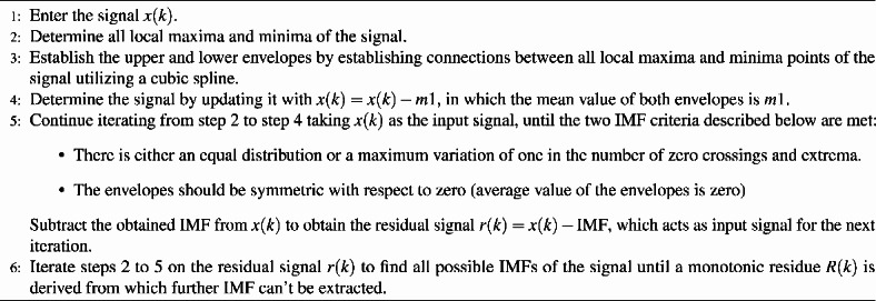
Empirical Mode Decomposition (EMD) Algorithm⁶⁰

One of the biggest drawbacks of the EMD approach is frequent mode mixing. To address this issue, an enhanced noise-assisted approach-EEMD⁶² is developed to add distinct white noise to the original signal several times. Thus, the signal in the trial after adding white noise can be represented as:

8

where l is number of trials, is the white noise in the trial with zero mean and unit variance and is the amplitude of white noise.

EMD is performed for each trial, and finally, the IMF components are the mean of the ensembles of all the trials. The mean IMF component can be defined as:

9

However, the numerous white noises introduced by the EEMD approach are not completely eradicated after the averaging phase. To address this issue, Torres et al.⁶³ developed the complete ensemble empirical mode decomposition (CEEMDAN), which recovers the IMFs by using adaptive white noise, resulting in a perfect restoration of the original signal. The CEEMDAN technique calculates the initial residual signal, , as:

10

where is the first average IMF obtained by EEMD. The second average IMF is obtained as:

11

After finding the th residue , the IMF for the iteration can be found by:

12

where is an operator to extract the IMF from the given signal by the EMD algorithm, while amplitude denotes the signal-to-noise ratio (SNR) at each stage. The loop proceeds until a final monotonous residual signal is obtained, preventing further IMF extraction. The primary time series can now be represented as a summation of all IMFs and residue as

13

Hence, CEEMDAN can control the amount of noise during each decomposition phase and provide IMFs that can almost eliminate noise while reconstructing the original data. In short, CEEMDAN outperforms EEMD and EMD due to its greater decomposition efficiency and reduced reconstruction error.

Permutation entropy (PE)

Generally, the number of IMF components derived by the CEEMDAN algorithm will increase as the complexity of the input signal increases. To minimize the excessive CEEMDAN decomposition and thereby computational challenges, the CEEMDAN-deconstructed IMFs can be reconstructed using well-defined time series complexity analysis methods. Bandt et al.⁶⁷ suggested Permutation Entropy (PE) as a way for analyzing the complexity, dynamics and unpredictability of the time series. It offers numerous advantages, including high time sensitivity, simple and consistent calculation, and outstanding anti-noise performance. To improve the computational efficency, IMFs can be restructured according to the PE value. The basic algorithm for PE is discussed here:

1. First, a delay vector is created for each IMF () by phase space reconstruction to obtain the phase space delay vector :

   14

   where and denote the delay time and embedding dimension, respectively. indicates the number of samples in each delay vector, whereas specifies the distance between the sample points in the delay vector.
2. The elements in each delay vector are rearranged in increasing order of sample point values:

   15

   If , then their original positions can be sorted based on the value of , for example, if , then .
3. A collection of ordinal pattern sequences , which is one out of possibilities, can be constructed for each delay vector of the IMF of the series :

   16
4. Calculate the probability distribution of each ordinal pattern obtained for each delay vector. Further the normalized PE can be computed as:

   17

   The value of normalized PE () is between 0 and 1. A signal with greater complexity is represented by a larger value, and a stable, less complicated signal is represented by a lower number.

Whale optimization algorithm (WOA)

WOA was introduced by S. Mirjalili et al. in 2016, drawing motivation from the hunting behavior of whales. The algorithm consists of three stages: encircling the prey, spiral bubble-net feeding, and pursuing the prey. Every whale in the group exhibits two distinct behaviors during the hunting phase. One behavior is to encircle the prey, with all the whales converging towards each other. The second behavior involves the use of a bubble net, where the whales swim in a circular, shrinking spiral, releasing bubbles to disperse the prey. Whales will engage in these two hunting methods randomly while hunting, to encircle their target.

Encircling prey

Once the whales locate their prey, they initially surround it. The optimal whale location in WOA is the optimum prey location or a close proximity to it, due to the initial uncertainty regarding the optimal position. The remaining whales will endeavor to update their location to reach the prey in each succeeding iteration until a predetermined iteration is reached. Equations (18)-(22) provide a mathematical description of this encircling prey technique:

18

19

20

21

22

where represents the fittest whale position and represents the th search agent/whale position in the th iteration; is a random number between [0,1]; parameter ‘a’ linearly drops from 2 to 0 throughout the course of iterations; is the present iteration; is the defined maximum number of iterations; and are the control parameters computed as in equations (21) and (22).

The parameter signifies the interaction between the fittest whale and its prey. The whale location element is constantly updated by control parameters, and as more whales approach the leader whale, Various positions with respect to the ideal search agent can be acquired by modifying the coefficients A and C. Notably, every location between the critical points of search space becomes accessible through the inclusion of the random variable ’’ in the modelling.

Bubble-net spiral feeding procedure

Another hunting strategy used by whales is to approach the prey by evaluating the distance between them. They trap the prey when it reaches near them by spitting spiral bubbles, which is modelled by equation (24) which represents the distance between the present whale and best whale position as in equation (23):

23

24

Spiral bubble net feeding and encircling prey are two concurrent behaviors that occur during hunting. The ensuing numerical model exemplifies these natural activities by providing the spiral position updating and shrinking encircling mechanisms with a 50% chance of updating the whale position in each cycle, where p is a random variable in the range [0, 1]:

25

26

Furthermore, when employing the bubble-net strategy, whales expand their search zone and explore beyond local optima in an arbitrary pursuit of the prey.

Prey search

During the prey-seeking stage, individual whales modify their location in subsequent iterations by utilizing position information gathered from each other as a result of the random walking process during whale group hunting. Random search enhances the global optimization efficacy of the algorithm. In the equation (28), a mathematical description of this prey seeking stage is provided:

27

28

where denotes a randomly selected whale from the present population.

The convergence factor governs the update strategy. The whale performs the bubble net mode when , while the whale engages the prey encircling when in order to prevent stumbling into the local optimal.

Each WOA iteration launches with a predetermined set of random whale positions. Each whale, comprising the swarm, updates its position according to the Equation (28). An effective local-global search is achieved due to the adaptable convergence factor that facilitates the transition from encircling prey to spiral bubble net preying behavior. In addition, WOA is relatively straightforward to implement in practice, requiring only the modification of a few significant parameters. The WOA algorithm can achieve rapid convergence and also prevent falling into local optima during the iterative process.

Proposed non-linear dimension learning-based hunting whale optimization algorithm (NDLHWOA)

Complex optimization applications pose significant challenges to any meta-heuristic optimization. According to the literature, no optimization strategy can provide the optimal solution for all types of complex problems. Despite its versatility and simplicity, WOA is hampered by several drawbacks, including an imbalance between exploration and exploitation, an inadequately diverse population, and premature convergence. In order to address these issues, we propose an enhanced version of the WOA by incorporating the merits of the non- linear control parameter and the Dimension learning hunting (DLH) search strategy.

Methodology incorporated for enhancing WOA

Nonlinear control parameter

In WOA, as discussed, the adaptive values of ‘a’ and ‘A’ steer the shift from exploration to exploitation. In conventional WOA, half of the iterations are utilized on exploration () and the other half on exploitation (), as in Figure 1. In general, greater exploration of the search space leads to a lesser risk of local optimization stagnation. Figure 1 illustrates how to increase the exploration rate by using exponential functions instead of linear functions to reduce the parameter ‘a’ over the iterations. Excessive exploration leads to randomness and poor optimization results. However, over-exploitation reduces randomness. Furthermore, the linear decrement technique for parameter ’a’ fails to adequately describe the complex and unanticipated optimization process. This study presents an iterative non-linear exponential decay control strategy, as illustrated in the equation (29), with the aim of enhancing the optimal progression of WOA by updating the parameter ’a’.

29

The exponential decay function is employed to ascertain the required number of iterations for exploration and exploitation, which are 70% and 30% respectively (see Figure 1). Numerical results pertaining to test functions demonstrate that the non-linear approach outperforms the linear decreasing strategy in terms of enhancing the optimization capabilities of the algorithm.

Fig. 1.

Variation of parameter ’a’ value in conventional WOA and with exponential decay approach presented in this study.

Dimension learning hunting (DLH) search strategy

In WOA, a new position is allocated to each whale with the assistance of the dominant whale in the population. Consequently, there is a high chance that whales get entrapped in the local optima and the population prematurely loses diversity, leading to delayed convergence. In order to rectify these shortcomings, the proposed algorithm integrates the Dimension Learning Hunting (DLH) search technique, which involves neighboring learning algorithms, considering the individual hunting behavior of whales. DLH search agents acquire knowledge from the best positions and randomly selected search members in varied neighborhoods. For the current position , a new position is formulated by the conventional WOA algorithm, while another candidate is formulated by the DLH search strategy, as in equation (32). The Euclidean distance between the current location and the candidate point establishes the neighborhood radius .

30

The neighbors of indicated by are then formed using Equation (31) with regard to radius , where is the Euclidean distance between and randomly selected whale from the population:

31

Upon generating the neighborhood of , multi-neighbors learning is conducted according to equation (31), where the d-th index of is determined by utilizing the d-th index of a random neighbor chosen from and a random whale chosen from the population.

32

The best candidate is determined by comparing fitness values of the two positions, and , using equation (33):

33

After completing this process for each whale in the population for a particular iteration, continue the search until the desired number of iterations () of the algorithm is attained.

Considering the merits, an enhanced version of the whale optimization algorithm, the non-linear dimension learning-based hunting-based whale optimization algorithm (NDLHWOA), is proposed by incorporating the merits of the non-linear control parameter and DLH search strategy. Figure 2 displays the pseudo-code for the suggested approach.

Fig. 2.

Flow diagram of NDLHWOA.

Evaluation of NDLHWOA using benchmark functions

Every new optimization technique must first be examined using a series of mathematical functions to evaluate the performance improvement. This section evaluates the suggested Enhanced Whale Optimization algorithm using two multimodal functions, Griewank and Pendalized, and three unimodal functions, Sphere, Schwefel 2.21, and RosenBrock, with a dimension of 30. Table 1 contains information on the various mathematical functions used. The suggested algorithm was tested 10 times for each benchmark function on a population of 30. Multimodal benchmark functions provide a testing framework for exploration behavior as they contain multiple optimal solutions, whereas unimodal benchmark functions are most suitable for assessing exploitation due to a single optimum. The methods proposed in this paper are contrasted with the conventional WOA and the DLH-Based Whale Optimization Algorithm (DLHWOA) with respect to the benchmark functions outlined earlier. All experiments were done on an Intel Core (TM) i5-1235U 1.30 GHz CPU with 16.00 GB of RAM using MATLAB R2022b. Table 2 shows the experimental statistical findings, such as mean runtime and mean value. To provide a more thorough analysis of the convergence rate, Figure3 additionally displays the convergence curves of all the algorithms considered. Table 2 clearly indicates that NDLHWOA is quite competitive with other versions of WOA, both in unimodal and multimodal functions, proving very good exploitation and exploration capabilities and expanding their potential for application in a range of complicated real-time optimizations.

Table 1.

Mathematical functions used for validation.

Functions	Name	Equations	Dim. (D)	Range	Min. ideal value
Unimodal functions	Sphere		30	[−100,100]	0
	Schwefel 2.21		30	[−100,100]	0
	RosenBrock		30	[−30,30]	0
Multimodal functions	Griewank		30	[−600,600]	0
	Pendalized	f(x) = ++	30	[−50,50]	0

Table 2.

Analytical findings of various optimizations on mathematical functions.

Unimodal Function	Method	Mean Runtime (s)	Mean	Multimodal Function	Method	Mean Runtime (s)	Mean
Sphere	WOA	11.4	3.26E-73	Griewank	WOA	9.82	0.026528
	DLHWOA	19	4.20E-75		DLHWOA	20.84	0.005002
	NDLHWOA	18.67	1.81E-75		NDLHWOA	22.15	0.003615
Schwefel 2.21	WOA	9.2	38.66612	Pendalized	WOA	11.05	0.630826
	DLHWOA	18.58	1.169218		DLHWOA	22.19	0.066387
	NDLHWOA	18.66	0.712855		NDLHWOA	24.14	0.026549
RosenBrock	WOA	9.6	38.66612
	DLHWOA	19.29	1.169218
	NDLHWOA	18.94	0.712855

Fig. 3.

Comparative analysis of the convergence curves of the suggested algorithms with other algorithms over various mathematical functions.

Proposed CEEMDAN-PE-NDLHWOA-RELM framework for forecasting

As discussed earlier, an efficient optimization method can aid in the fine-tuning of the RELM model parameters to overcome its limitations and boost its efficacy. In this paper, the proposed whale optimization technique, NDLHWOA, is effectively utilized to prune various RELM parameters for forecasting applications. Since the intermittent features and heavy noise characteristics of datasets significantly limit prediction accuracy, an efficient decomposition technique, namely CEEMDAN, can be utilized to break down datasets into less complex signals. Further, to reduce over-decomposition and computational weight, PE was utilized to calculate the complexity of the IMFs and recombine them into a new sub-series IMFn, according to the PE value. Finally, a NDLHWOA RELM-based forecast model is created for each sub-series aggregating prediction results for all components to get the final prediction result. The forecasting approach flow is shown in Figure 4. The primary steps of the framework are data collection, pre-processing, design and training of the RELM model, prediction, and performance evaluation.

Fig. 4.

Proposed CEEMDAN-PE-NDLHWOA-RELM framework.

Data acquisition

The experiment used a one-year meteorological dataset collected from a weather station located at Kasavanahalli, Bengaluru, Karnataka, India. (Figure 5) from December 1, 2020 to November 30, 2021⁴⁸. This study extends the proposed paradigm to four different seasons-Dec-Feb, Mar-May, June-Aug, and Sept-Nov-to illustrate its adaptability and advantages. Wind speed and solar irradiation are the two meteorological factors used in the datasets for prediction, as shown in Figure 6 and Figure 7. Table 3displays statistical information about the considered datasets⁴⁸.

Fig. 5.

a) Site location b) Weather station used in this study.

Fig. 6.

Wind speed data for the entire predicted period.

Fig. 7.

Solar irradiance data for the entire predicted period.

Table 3.

Statistical information of the datasets considered⁴⁸.

Dataset	Time period	No of samples	Parameter	Max Value	Min Value	Std.Dev	Mean
Dataset 1	Dec 1st, 2020 to Feb 28th, 2021	2160	Solar irradiance (W/)	994.74	0	295.005	210.097
			Wind speed (m/s)	10.59	0.33	1.759	5.42
Dataset 2	Mar 1st, 2021 to May 31st, 2021	2208	Solar irradiance (W/)	1026	0	337.999	263.014
			Wind speed (m/s)	11.13	0.1	2.049	5.164
Dataset 3	June 1st, 2021 to Aug 31st, 2021	2208	Solar irradiance (W/)	968	0	264.081	206.077
			Wind speed (m/s)	14.59	0.21	2.538	6.66
Dataset 4	Sep 1st, 2021 to Nov 30th, 2021	2184	Solar irradiance (W/)	925.44	0	258.398	189.610
			Wind speed (m/s)	11.8	0.15	2.042	5.039

Data decomposition by CEEMDAN-PE

Pre-processing is essential for any forecast model since data quality has a substantial influence on model performance. First, the missing values in the complete dataset are substituted with the mean values. Individual time series are then deconstructed using an effective decomposition algorithm. Figure 8 and Table 4 exhibit a comparison of the decomposition results using EMD, EEMD, and CEEMDAN on the given time series. This comparison is based on the reconstruction error, which measures the RMSE between the original series and the sum of the related IMFs. Table 4 shows that the EEMD strategy has the highest reconstruction error when compared to other approaches, showing insufficient decomposition. Results clearly indicate that the CEEMDAN algorithm outperforms other methods in terms of decomposition and reconstruction accuracy. In this study,individual time series are deconstructed using the CEEMDAN technique. Specifically, in CEEMDAN, 500 groups of white noise signals with a non-standard deviation of 0.2 are added in each trial to derive the IMF components. Figure9 shows the decomposition results of CEEMDAN on wind speed and solar irradiance series for all datasets. Further, PE [delay ()=1, embedding function(m)=3] is employed to quantify the intricacy of every IMF. To minimize decomposition and computational complexity, similar entropy IMF components are added to create the recombination component IMFn, as illustrated in Table 5. Fig 10 shows the recombination sequences for all datasets considered.

Fig. 8.

Reconstruction error with EMD, EEMD, and CEEMDAN algorithms for wind speed and solar irradiance decomposition of Dataset-2.

Table 4.

Reconstruction error with Decomposition algorithms.

Reconstruction Error
	Dataset-1		Dataset-2		Dataset-3		Dataset-4
	Wind speed (m/s)	Solar irradiance (W/)	Wind speed (m/s)	Solar irradiance (W/)	Wind speed (m/s)	Solar irradiance (W/)	Wind speed (m/s)	Solar irradiance (W/)
EMD	5.56E-16	4.89E-14	5.72E-16	6.42E-14	6.91E-16	4.73E-14	6.25E-16	4.69E-14
EEMD	5.050682653	186.7064598	5.158044442	221.2696068	6.922766288	200.8776121	4.287499526	134.7117934
CEEMDAN	2.63E-16	3.81E-15	2.79E-16	8.45E-15	2.80E-16	4.14E-15	2.80E-16	4.02E-15

Fig. 9.

CEEMDAN decomposition of wind speed and solar irradiance series for all datasets.

Table 5.

Recombinant sequences for all datasets.

Dataset	IMF	Permutation Entropy (PE)	Recombination	IMFn	Dataset	IMF	Permutation Entropy(PE)	Recombination	IMFn
Dataset-1 Wind Speed	IMF 1	0.851966	IMF 1	IMFn 1	Dataset-1 Solar irradiance	IMF 1	0.839571	IMF 1	IMFn 1
	IMF 2	0.667912	IMF 2	IMFn 2		IMF 2	0.69977	IMF 2	IMFn 2
	IMF 3	0.560364	IMF 3	IMFn 3		IMF 3	0.578319	IMF 3	IMFn 3
	IMF 4	0.47334	IMF 4	IMFn 4		IMF 4	0.484967	IMF 4	IMFn 4
	IMF 5	0.426341	IMF 5 + IMF6 + IMF 7 + IMF 8	IMFn 5		IMF 5	0.440668	IMF 5 + IMF 6 + IMF 7 + IMF 8	IMFn 5
	IMF 6	0.408371				IMF 6	0.398813
	IMF 7	0.381838				IMF 7	0.39497
	IMF 8	0.38794				IMF 8	0.390869
Dataset-2 Wind Speed	IMF 1	0.846801	IMF 1	IMFn 1	Dataset-2 Solar irradiance	IMF 1	0.856873	IMF 1	IMFn 1
	IMF 2	0.630293	IMF 2	IMFn 2		IMF 2	0.691547	IMF 2	IMFn 2
	IMF 3	0.532002	IMF 3	IMFn 3		IMF 3	0.568826	IMF 3	IMFn 3
	IMF 4	0.460399	IMF 4	IMFn 4		IMF 4	0.487463	IMF 4	IMFn 4
	IMF 5	0.422975	IMF 5 + IMF 6 + IMF 7 + IMF 8	IMFn 5		IMF 5	0.439967	IMF 5 + IMF 6 + IMF 7 + IMF 8	IMFn 5
	IMF 6	0.403354				IMF 6	0.414698
	IMF 7	0.379867				IMF 7	0.398416
	IMF 8	0.367873				IMF 8	0.390942
Dataset-3 Wind Speed	IMF 1	0.884131	IMF 1	IMFn 1	Dataset-3 Solar irradiance	IMF 1	0.854714	IMF 1	IMFn 1
	IMF 2	0.67582	IMF 2	IMFn 2		IMF 2	0.690856	IMF 2	IMFn 2
	IMF 3	0.558486	IMF 3	IMFn 3		IMF 3	0.569243	IMF 3	IMFn 3
	IMF 4	0.475766	IMF 4	IMFn 4		IMF 4	0.497502	IMF 4	IMFn 4
	IMF 5	0.428302	IMF 5 + IMF 6 + IMF 7 + IMF 8	IMFn 5		IMF 5	0.44832	IMF 5 + IMF 6 + IMF 7 + IMF 8	IMFn 5
	IMF 6	0.400871				IMF 6	0.419134
	IMF 7	0.381361				IMF 7	0.401316
	IMF 8	0.369258				IMF 8	0.390771
Dataset-4 Wind Speed	IMF 1	0.885983	IMF 1	IMFn 1	Dataset-4 Solar irradiance	IMF 1	0.878438	IMF 1	IMFn 1
	IMF 2	0.681884	IMF 2	IMFn 2		IMF 2	0.698845	IMF 2	IMFn 2
	IMF 3	0.561305	IMF 3	IMFn 3		IMF 3	0.573622	IMF 3	IMFn 3
	IMF 4	0.488607	IMF 4	IMFn 4		IMF 4	0.480983	IMF 4	IMFn 4
	IMF 5	0.43016	IMF 5 + IMF 6 + IMF 7 + IMF 8	IMFn 5		IMF 5	0.427382	IMF 5 + IMF 6 + IMF 7 + IMF 8	IMFn 5
	IMF 6	0.401709				IMF 6	0.396334
	IMF 7	0.399589				IMF 7	0.385015
	IMF 8	0.391426				IMF 8	0.388504

Fig. 10.

Recombination results for the CEEMDAN-PE deconstructed datasets.

Model optimization and forecasting

Normalizing the data boosts model performance since the activation function is more sensitive to input variables. So, at first, all IMFs are standardized with the Min-Max scaler. Subsequently, the normalized data is partitioned into two distinct sets: test 20% and train 80%. Due to the fact that distinct signals possess unique qualities, a single model is unable to handle every characteristic of all the IMFns. Consequently, a cluster of RELMs with diverse hyperparameters is employed separately for forecasting different IMFs with different characteristics. This work uses NDLHWOA to trim RELM parameters, including input-hidden layer weights, biases, activation functions, hidden layer neurons, and regularization parameters that define the whale positions in the NDLHWOA algorithm. This method will effectively evaluate the RELM model for various parameter value combinations. Table 6 lists the RELM parameter ranges. The NDLHWOA algorithm parameters are listed in Table 7.

Table 6.

RELM parameter ranges.

RELM parameter	Range
Input-hidden layer weights (w)	[−1,1]
Input-hidden layer Bias (b)	[0,1]
Hidden layer neurons(n)	[10,200]
Activation Function	[’relu’, ’leaky relu’,’sin’,’sigmoid’,’tanh’]
Regularization parameter (C)	[,]

Table 7.

Configuration of NDLHWOA algorithm parameters.

NDLHWOA parameter	Value
Maximum iterations	200
Whale population	20
random vector (r)	[0,1]
a	decreased nonlinearly from 2 to 0 throughout the iterations

Given that time series prediction requires model performance, the RMSE between forecasted and actual values serves as the fitness function for determining the optimal whale location. Thus, final output weights are computed for each robust RELM model of the IMFn, and all parameter values are effectively updated in each iteration. The final stage consists of merely adding the predicted values of each IMFn component.

Assessment criteria

Performance evaluation is essential for validating any model. In order to showcase the reliability, precision, and user-friendly predictive capabilities of the proposed model, as well as to evaluate its performance in comparison to other models, we utilized the assessment metrics outlined in Table 8. where the actual and predicted values are and , respectively, at time t. represents the mean value among all values examined. In order to evaluate the precision and consistency of our hybrid forecasting model, we conducted a comparison of its root mean square error (RMSE) with other models using the percentage decrease in RMSE ( ), as defined in equation (34)⁴⁸:

34

Table 8.

Assessment criteria.

Assessment criteria	Explanation	Equation
MSE	Mean Square Error
-score	Coefficient of Determination
RMSE	Root Mean Square Error
MAE	Mean Absolute Error

Results and comparative analysis

The prediction ability and performance of the proposed model are evaluated versus six existing models: WOA-SVR, WOA-LSTM, WOA-RELM, DHLWOA-RELM, and NDLHWOA-RELM. Table 9 provides details regarding the configuration parameters of benchmark models.

Table 9.

Configuration Model Parameters.

Forecasting models	Model Parameters		WOA Parameters
	Parameter	Value	Parameter	Value
WOA-SVR	Kernel	Radial basis function (RBF)	random vector (r)	[0,1]
	Cost	[0.001,10]
	Gamma	[0.001,10]	a	Decreased linearly from 2 to 0 throughout the iterations.
WOA-LSTM	No. of Hidden layers	[1,4]	Maximum number of iterations	200
	Hidden layer Cells	[10,200]
	Batch Size	[10,200]
WOA-RELM	Input-hidden layer weights (w)	[−1,1]
	Input-hidden layer Bias (b)	[0,1]
	Hidden layer Neurons (n)	[10,200]
DLHWOA-RELM	Activation Function	[’relu’,leaky relu’, ’sin’, ’sigmoid’, ’tanh’]
NDLHWOA-RELM			Random vector (r)	[0,1]
			a	Decreased nonlinearly from 2 to 0 throughout the iterations.
			Maximum number of iterations	200

Case Study-1 wind speed forecasting

In this case study, the wind speed data from all datasets is utilized to perform one-hour-ahead short-term wind speed forecasting using the proposed model. Table 9 examines the forecasting accuracy of various models in one-step forward wind speed prediction with different statistical error indices [bold font represents the least errors]. Figure 11 shows the one-step-ahead wind speed prediction curves produced by the various models for the datasets being evaluated. Figure12 shows a comparison of several wind speed forecasting models using RMSE and MAE values. Fig. 13 illustrates how the proposed CEEMDAN-PE-NDLHWOA RELM model surpasses the regular WOA-RELM model in terms of percentage reduction in root mean square error (PRMSE). Figure14 illustrates the scatter plot of the proposed model in wind speed forecasting for all datasets considered. The experimental findings are summarized as follows:

• The forecast models for dataset 3 demonstrate relatively low error levels as measured by MAE and RMSE, suggesting that the accuracy depends on the dataset and technique being used.

• For all the datasets considered, the WOA-optimized RELM model outperforms WOA-SVR and WOA-LSTM in terms of learning and prediction, validating its usage in prediction models.

• Clearly, results prove that improvising the conventional WOA with a dimension learning hunting strategy (DLH) and non-linearity has a considerable impact on optimizing RELM parameters, as there is a 0.57% to 5.596% percentage reduction in RMSE for various datasets considered, as shown in Figure13.

• Among the six forecasting models studied, the proposed CEEMDAN-PE-NDHLWOA-RELM has greater prediction accuracy for all four datasets considered, as highlighted in Table 10. This demonstrates that the use of the decomposition methodology (CEEMDAN-PE) can significantly improve prediction accuracy.

  1. The RMSE and MAE of the suggested framework for dataset-1 are 0.317224 m/s and 0.242096 m/s, respectively, resulting in a percentage reduction in RMSE of 23.80% when compared to the conventional WOA-RELM.
  2. Meanwhile, the proposed model’s RMSE and MAE values for dataset-2 are 0.222569 m/s and 0.173767 m/s, respectively, resulting in a percentage reduction in RMSE of 37.38% when compared to the conventional WOA-RELM.
  3. For dataset-3, the RMSE and MAE of our model are 0.209091 m/s and 0.153769 m/s, respectively, resulting in a percentage reduction in RMSE of 33.92% when compared to the conventional WOA-RELM.
  4. For dataset-4, the RMSE and MAE of the proposed framework are 0.237373 m/s and 0.176232 m/s, respectively, resulting in a percentage reduction in RMSE of 34.14% when compared to the conventional WOA-RELM.

Fig. 11.

Wind speed prediction curves derived by the various models for all datasets.

Fig. 12.

Comparison of different models based on RMSE and MAE for wind speed forecasting.

Fig. 13.

Comparison of models based on for wind speed forecasting.

Fig. 14.

Scatter plot of the proposed model in wind speed forecasting for all dataset.

Table 10.

Statistical error metrics for one-step forward wind speed prediction for diverse datasets.

Dataset-1					Dataset-2
MODEL	MSE[/]	R2	RMSE[m/s]	MAE[m/s]	MODEL	MSE[/]	R2	RMSE[m/s]	MAE[m/s]
WOA-SVR	0.186584	0.961784	0.431953	0.310532	WOA-SVR	0.134445	0.947855	0.366667	0.258738
WOA-LSTM	0.183556	0.962404	0.428434	0.315414	WOA-LSTM	0.138213	0.946394	0.371770	0.258835
WOA-RELM	0.173319	0.964501	0.416316	0.292733	WOA-RELM	0.126320	0.951006	0.355415	0.254975
DLHWOA-RELM	0.154754	0.968303	0.393388	0.277170	DLHWOA-RELM	0.116817	0.954692	0.341786	0.246462
NDLHWOA-RELM	0.156203	0.968006	0.395225	0.286198	NDLHWOA-RELM	0.11679	0.95470	0.341750	0.24646
Proposed model	0.100631	0.979389	0.317224	0.242096	Proposed model	0.049537	0.980787	0.222569	0.173767

Dataset-3					Dataset-4
MODEL	MSE[/]	R2	RMSE[m/s]	MAE[m/s]	MODEL	MSE[/]	R2	RMSE[m/s]	MAE
WOA-SVR	0.127900	0.968576	0.357631	0.274307	WOA-SVR	0.139775	0.966497	0.373865	0.255214
WOA-LSTM	0.127384	0.968702	0.356908	0.253628	WOA-LSTM	0.137461	0.967051	0.370757	0.249566
WOA-RELM	0.100126	0.975399	0.316427	0.225703	WOA-RELM	0.129899	0.968864	0.360416	0.244223
DLHWOA-RELM	0.098991	0.975678	0.314628	0.228461	DLHWOA-RELM	0.114865	0.972077	0.338917	0.229311
NDLHWOA-RELM	0.098979	0.975681	0.314610	0.227812	NDLHWOA-RELM	0.114865	0.972077	0.338917	0.229311
Proposed model	0.043719	0.989258	0.209091	0.153769	Proposed model	0.056346	0.983825	0.237373	0.176232

Case study-II solar irradiance forecasting

This case study glances at the ability of the proposed model to predict one-hour-ahead solar irradiance for all datasets. Table 10 compares all the solar irradiance forecast models using different statistical error indices. Figure15 displays the solar irradiance prediction curves produced by different models for all the datasets, specifically for one-step-ahead predictions. Figure16 illustrates a comparison between various models based on RMSE and MAE for solar irradiance predictions.Figure17 illustrates the enhanced computational performance of the CEEMDAN-PE-NDLHWOA-RELM model compared to the WOA-RELM model, measured in terms of PRMSE.Figure18 illustrates the scatter plot of the proposed model in solar irradiance forecasting for all datasets considered. The experimental findings are summarized as follows:

• Compared to other datasets, the prediction models for dataset-2 exhibit low error levels based on MAE and RMSE, indicating that accuracy varies by dataset and forecast model considered.

• For all the datasets considered, the WOA-optimized RELM model outperforms WOA-SVR and WOA-LSTM in terms of learning and prediction, validating its usage in prediction models.

• Clearly, results prove that improvising the conventional WOA with DLH strategy and non-linearity has a considerable impact on optimizing RELM parameters, as there is a 0.67% to 4.97% percentage reduction in RMSE for various datasets considered, as shown in Figure17.

• Among the six forecasting models studied, the proposed CEEMDAN-PE-NDHLWOA-RELM has greater prediction accuracy for all four datasets considered, as highlighted in Table 11. This demonstrates that the decomposition methodology (CEEMDAN-PE) can substantially improve the accuracy of predictions.

  1. The RMSE and MAE of the proposed framework for dataset-1 are 23.21074 and 14.13455 , respectively, resulting in a percentage reduction in RMSE of 8.0% when compared to the conventional WOA-RELM.
  2. Meanwhile, the proposed model’s RMSE and MAE values for dataset-2 are 22.71806 and 17.24666 , respectively, resulting in a percentage reduction in RMSE of 34.40% when compared to the conventional WOA-RELM.
  3. For dataset dataset-3, the RMSE and MAE of the proposed framework are 27.51491 and 20.58895 , respectively, resulting in a percentage reduction in RMSE of 12.73% when compared to the conventional WOA-RELM.
  4. For dataset-4, the RMSE and MAE of our model are 24.69961 and 18.85851 , respectively, resulting in a percentage reduction in RMSE of 26.41% when compared to the conventional WOA-RELM.

Fig. 15.

Solar Irradiance prediction curves derived by the various models for all Datasets.

Fig. 16.

Comparison of solar irradiance forecasting models based on RMSE and MAE.

Fig. 17.

Comparison of models based on for solar irradiance predictions.

Fig. 18.

Scatter plot of the proposed model in solar irradiance forecasting for all datasets.

Table 11.

Statistical error metrics for one-step forward solar irradiance prediction for diverse datasets.

Dataset-1					Dataset-2
MODEL	MSE[/]	R2	RMSE[W/]	MAE[W/]	MODEL	MSE[/]	R2	RMSE[W/]	MAE[W/]
WOA-SVR	1085.14726	0.99041	32.94157	26.86358	WOA-SVR	1565.03356	0.984252	39.560505	28.193034
WOA-LSTM	749.35069	0.99337	27.37427	16.22632	WOA-LSTM	994.52428	0.98999	31.53608	19.00940
WOA-RELM	636.55652	0.99526	25.23007	14.76210	WOA-RELM	1199.4978	0.98793	34.63377	21.70615
DLHWOA-RELM	621.82638	0.99450	24.93645	15.65122	DLHWOA-RELM	1134.2687	0.98859	33.67891	21.18271
NDLHWOA-RELM	577.95020	0.99489	24.04059	15.36271	NDLHWOA-RELM	1083.2534	0.98910	32.91282	21.25829
Proposed model	538.73842	0.99524	23.21074	14.13455	Proposed model	516.11032	0.99481	22.71806	17.24666

Dataset-3					Dataset-4
MODEL	MSE[/]	R2	RMSE[W/]	MAE[W/]	MODEL	MSE[/]	R2	RMSE[W/]	MAE[W/]
WOA-SVR	1291.99911	0.98252	35.94439	26.14617	WOA-SVR	1402.2157	0.97503	37.44617	27.00022
WOA-LSTM	1119.54211	0.98485	33.45956	20.28611	WOA-LSTM	1080.8597	0.98075	32.87643	19.80148
WOA-RELM	994.00374	0.98655	31.52782	19.69420	WOA-RELM	1126.4302	0.97994	33.56233	20.79101
DLHWOA-RELM	1022.57330	0.98616	31.97770	21.06476	DLHWOA-RELM	1110.5942	0.98022	33.32558	20.40784
LNDLHWOA-RELM	1007.36995	0.98637	31.73909	20.12761	NDLHWOA-RELM	1154.9671	0.97943	33.98481	21.38221
Proposed model	757.07014	0.98976	27.51491	20.58895	Proposed model	610.07087	0.98913	24.69961	18.85851

Conclusion

Driven by contemporary advancements in hybrid forecasting methodology, a novel hybrid CEEMDAN-PE-NDLHWOA- RELM model has been proposed in this article for wind speed and solar irradiance forecasting. As discussed, an effective decomposition method, the CEEMDAN-PE approach, was employed to partition datasets into simpler signals to address the intermittent and noisy nature of the datasets. The proposed hybrid model utilizes NDLHWOA to refine RELM to model each reconstructed signal component. Case studies of seasonal wind speed and solar irradiance data acquired from a meteorological station in Kasavanahalli, Bengaluru, Karnataka, India, are used to demonstrate the stability and precision of the combined model. The effectiveness of the model as a competitive technology in forecasting is demonstrated by the outcomes of the comparison with five other established benchmark models using a variety of evaluation metrics. However, the ensuing limitations of the suggested hybrid forecast model may provide opportunities for further research.

• The primary focus of the proposed research is a univariate prediction model that excludes the inclusion of any other correlated features as input variables for modeling. In the future, correlated input features such as pressure, temperature, humidity, and wind direction can be integrated into the modeling, leading to a multivariate RELM model. Subsequent investigations may also assess the effectiveness of the newly developed models.

• In order to enhance the precision of predictions even further, an appropriate error correction algorithm may be developed for post-processing and mitigating forecast errors. The effectiveness of the proposed model incorporating error correction algorithms may be deeply analyzed.

Abbreviations

RES

Renewable Energy sources

PV

Photovoltaic

IMF

Intrinsic mode function

EMD

Empirical Mode Decomposition

EEMD

Enhanced Empirical Mode Decomposition

CEEMD

Complete Ensemble Empirical Mode Decomposition

CEEMDAN

Complete Ensemble Empirical Mode Decomposition with Adaptive Noise

PE

Permutation Entropy

WOA

Whale Optimization Algorithm

DLH

Dimension Learning Hunting

NDLHWOA

Nonlinear Dimension Learning Hunting Whale Optimization Algorithm

SLFFN

Single-Hidden-Layer Feedforward Neural Network

ELM

Extreme Learning Machines

RELM

Regularized Extreme Learning Machines

MSE

Mean Square Error

RMSE

Root Mean Square Error

MAE

Mean Absolute Error

R2 score

Coefficient of Determination

PRMSE

Percentage Decrease in RMSE

WOA-SVR

Whale Optimized Support Vector Regression

WOA-LSTM

Whale Optimized Long-Short-Term Memory

WOA-RELM

Whale Optimized Regularized Extreme Learning Machines

DHLWOA-RELM

Dimension Learning Hunting Whale Optimized Regularized Extreme Learning Machines

NDLHWOA-RELM

Nonlinear Dimension Learning Hunting Whale Optimized Regularized Extreme Learning Machines

Author contributions

All authors contributed to the study, conception, and design. all authors commented on the manuscript. All authors read and approved the final manuscript.

Funding

The authors did not receive support from any organisation for the submitted work.

Data availibility

The datasets used and/or analysed during the current study are available from the corresponding author upon reasonable request.

Declarations

Competing interests

The authors declare no competing interests.

Consent for publication

Authors transfer to Springer the publication rights and warrant that our contribution is original.

References

- 1.Diéguez, M. S., Fattahi, A., Sijm, J., España, G. M. & Faaij, A. Modelling of decarbonisation transition in national integrated energy system with hourly operational resolution. Advances in Applied Energy3, 100043 (2021). [Google Scholar]
- 2.Jing, R., Zhou, Y. & Wu, J. Electrification with flexibility towards local energy decarbonization. adv appl energy 20225, 100088 (2022). [Google Scholar]
- 3.Council, G. W. E. Gwec global wind report 2023 (Bonn, Germany, Global Wind Energy Council, 2023). [Google Scholar]
- 4.Wang, J., Song, Y., Liu, F. & Hou, R. Analysis and application of forecasting models in wind power integration: A review of multi-step-ahead wind speed forecasting models. Renewable and Sustainable Energy Reviews60, 960–981 (2016). [Google Scholar]
- 5.Wang, Y., Zou, R., Liu, F., Zhang, L. & Liu, Q. A review of wind speed and wind power forecasting with deep neural networks. Applied Energy304, 117766 (2021). [Google Scholar]
- 6.Diagne, M., David, M., Lauret, P., Boland, J. & Schmutz, N. Review of solar irradiance forecasting methods and a proposition for small-scale insular grids. Renewable and Sustainable Energy Reviews27, 65–76 (2013). [Google Scholar]
- 7.Yang, B. et al. Classification and summarization of solar irradiance and power forecasting methods: A thorough review. CSEE Journal of Power and Energy Systems (2021).
- 8.Nie, Y., Zelikman, E., Scott, A., Paletta, Q. & Brandt, A. Skygpt: Probabilistic ultra-short-term solar forecasting using synthetic sky images from physics-constrained videogpt. Advances in Applied Energy14, 100172 (2024). [Google Scholar]
- 9.Paletta, Q. et al. Advances in solar forecasting: Computer vision with deep learning. Advances in Applied Energy 100150 (2023).
- 10.Lydia, M., Kumar, S. S., Selvakumar, A. I. & Kumar, G. E. P. Linear and non-linear autoregressive models for short-term wind speed forecasting. Energy conversion and management112, 115–124 (2016). [Google Scholar]
- 11.Mora-Lopez, L. & Sidrach-de Cardona, M. Multiplicative arma models to generate hourly series of global irradiation. Solar Energy63, 283–291 (1998). [Google Scholar]
- 12.Erdem, E. & Shi, J. Arma based approaches for forecasting the tuple of wind speed and direction. Applied Energy88, 1405–1414 (2011). [Google Scholar]
- 13.Nair, K. R., Vanitha, V. & Jisma, M. Forecasting of wind speed using ann, arima and hybrid models. In 2017 international conference on intelligent computing, instrumentation and control technologies (ICICICT), 170–175 (IEEE, 2017).
- 14.Yang, D., Ye, Z., Lim, L. H. I. & Dong, Z. Very short term irradiance forecasting using the lasso. Solar Energy114, 314–326 (2015). [Google Scholar]
- 15.Shakya, A. et al. Solar irradiance forecasting in remote microgrids using markov switching model. IEEE Transactions on sustainable Energy8, 895–905 (2016). [Google Scholar]
- 16.Jiang, Y., Long, H., Zhang, Z. & Song, Z. Day-ahead prediction of bihourly solar radiance with a markov switch approach. IEEE Transactions on Sustainable Energy8, 1536–1547 (2017). [Google Scholar]
- 17.Yadav, A. K. & Chandel, S. Solar radiation prediction using artificial neural network techniques: A review. Renewable and sustainable energy reviews33, 772–781 (2014). [Google Scholar]
- 18.Ekici, B. B. A least squares support vector machine model for prediction of the next day solar insolation for effective use of pv systems. Measurement50, 255–262 (2014). [Google Scholar]
- 19.Bae, K. Y., Jang, H. S. & Sung, D. K. Hourly solar irradiance prediction based on support vector machine and its error analysis. IEEE Transactions on Power Systems32, 935–945 (2016). [Google Scholar]
- 20.Ul Islam Khan, M. et al. Securing electric vehicle performance: Machine learning-driven fault detection and classification. IEEE Access12, 71566–71584 (2024). [Google Scholar]
- 21.Syama, S. & Ramprabhakar, J. Multistep ahead solar irradiance and wind speed forecasting using bayesian optimized long short term memory. In 2022 7th International Conference on Communication and Electronics Systems (ICCES), 164–171 (IEEE, 2022).
- 22.Meena, V., Singh, V. & Guerrero, J. M. Investigation of reciprocal rank method for automatic generation control in two-area interconnected power system. Mathematics and Computers in Simulation225, 760–778. 10.1016/j.matcom.2024.06.007 (2024). [Google Scholar]
- 23.Kumar, V. B., Nookesh, V. M., Saketh, B. S., Syama, S. & Ramprabhakar, J. Wind speed prediction using deep learning-lstm and gru. In 2021 2nd International Conference on Smart Electronics and Communication (ICOSEC), 602–607 (IEEE, 2021).
- 24.Meena, V., Singh, V. P., Padmanaban, S. & Benedetto, F. Rank exponent-based reduction of higher order electric vehicle systems. IEEE Transactions on Vehicular Technology73, 12438–12447. 10.1109/TVT.2024.3387975 (2024). [Google Scholar]
- 25.Balan, A., Ramanathan, T. et al. Comparative analysis of machine learning algorithms to predict solar irradiance. In 2022 International Conference on Disruptive Technologies for Multi-Disciplinary Research and Applications (CENTCON), vol. 2, 167–172 (IEEE, 2022).
- 26.Kumar, U., Chaganti, P. C. V., Syama, S. et al. Deep learning-based multistep forecasting for photovoltaic power generation: A comprehensive comparative study. In 2023 International Conference on Self Sustainable Artificial Intelligence Systems (ICSSAS), 408–413 (IEEE, 2023).
- 27.Lin, F., Zhang, Y., Wang, K., Wang, J. & Zhu, M. Parametric probabilistic forecasting of solar power with fat-tailed distributions and deep neural networks. IEEE Transactions on Sustainable Energy13, 2133–2147 (2022). [Google Scholar]
- 28.Lyu, Z., Shen, Y., Zhao, Y. & Hu, T. Solar radiation prediction based on conformer-glaplace-sdar model. Sustainability15, 15050 (2023). [Google Scholar]
- 29.Huang, G.-B., Zhu, Q.-Y. & Siew, C.-K. Extreme learning machine: a new learning scheme of feedforward neural networks. In 2004 IEEE international joint conference on neural networks (IEEE Cat. No. 04CH37541), vol. 2, 985–990 (Ieee, 2004).
- 30.Ding, S., Xu, X. & Nie, R. Extreme learning machine and its applications. Neural Computing and Applications25, 549–556 (2014). [Google Scholar]
- 31.Wang, J., Lu, S., Wang, S.-H. & Zhang, Y.-D. A review on extreme learning machine. Multimedia Tools and Applications81, 41611–41660 (2022). [Google Scholar]
- 32.Wang, Y., Zou, R., Liu, F., Zhang, L. & Liu, Q. A review of wind speed and wind power forecasting with deep neural networks. Applied Energy304, 117766 (2021). [Google Scholar]
- 33.Mathur, A. et al. Data-driven optimization for microgrid control under distributed energy resource variability. Scientific Reports14, 10806 (2024). [DOI] [PMC free article] [PubMed] [Google Scholar]
- 34.Nikolić, V. et al. Extreme learning machine approach for sensorless wind speed estimation. Mechatronics34, 78–83 (2016). [Google Scholar]
- 35.Nithara, P. et al. Brayton-moser passivity based controller for constant power load with interleaved boost converter. Scientific Reports14, 28325 (2024). [DOI] [PMC free article] [PubMed] [Google Scholar]
- 36.Ren, Y. Short-term wind power prediction based on extreme learning machine. In 2021 International Conference on Digital Society and Intelligent Systems (DSInS), 188–192 (IEEE, 2021).
- 37.Wang, L., Li, X. & Bai, Y. Short-term wind speed prediction using an extreme learning machine model with error correction. Energy Conversion and Management162, 239–250 (2018). [Google Scholar]
- 38.Liu, H., Mi, X. & Li, Y. Smart multi-step deep learning model for wind speed forecasting based on variational mode decomposition, singular spectrum analysis, lstm network and elm. Energy Conversion and Management159, 54–64 (2018). [Google Scholar]
- 39.Bouzgou, H. & Gueymard, C. A. Fast short-term global solar irradiance forecasting with wrapper mutual information. Renewable Energy133, 1055–1065 (2019). [Google Scholar]
- 40.Zhang, H., Ding, F., Wang, J., Zhang, R. & Guo, S. Optimized prediction of solar irradiation based on mpc and elm neural network. In IOP Conference Series: Earth and Environmental Science, vol. 512, 012164 (IOP Publishing, 2020).
- 41.Varshney, T. et al. Fuzzy analytic hierarchy process based generation management for interconnected power system. Scientific Reports14, 11446 (2024). [DOI] [PMC free article] [PubMed] [Google Scholar]
- 42.Zhu, Q.-Y., Qin, A. K., Suganthan, P. N. & Huang, G.-B. Evolutionary extreme learning machine. Pattern recognition38, 1759–1763 (2005). [Google Scholar]
- 43.Li, A. & Wei, X. Short-term wind speed forecasting based on pso-elm. In Innovative Computing: IC 2020, 1059–1063 (Springer, 2020).
- 44.Xiao, L., Qian, F. & Shao, W. Multi-step wind speed forecasting based on a hybrid forecasting architecture and an improved bat algorithm. Energy Conversion and Management143, 410–430 (2017). [Google Scholar]
- 45.Wu, C., Wang, J., Chen, X., Du, P. & Yang, W. A novel hybrid system based on multi-objective optimization for wind speed forecasting. Renewable energy146, 149–165 (2020). [Google Scholar]
- 46.Wang, J., Jiang, H., Wu, Y. & Dong, Y. Forecasting solar radiation using an optimized hybrid model by cuckoo search algorithm. Energy81, 627–644 (2015). [Google Scholar]
- 47.Boriratrit, S., Srithapon, C., Fuangfoo, P. & Chatthaworn, R. Metaheuristic extreme learning machine for improving performance of electric energy demand forecasting. Computers11, 66 (2022). [Google Scholar]
- 48.Syama, S., Ramprabhakar, J., Anand, R. & Guerrero, J. M. A hybrid extreme learning machine model with lévy flight chaotic whale optimization algorithm for wind speed forecasting. Results in Engineering19, 101274 (2023). [Google Scholar]
- 49.Mirjalili, S. & Lewis, A. The whale optimization algorithm. Advances in engineering software95, 51–67 (2016). [Google Scholar]
- 50.Mohammed, H. M., Umar, S. U., Rashid, T. A. et al. A systematic and meta-analysis survey of whale optimization algorithm. Computational intelligence and neuroscience2019 (2019). [DOI] [PMC free article] [PubMed]
- 51.Lian, L. & He, K. Ultra-short-term wind speed prediction based on variational mode decomposition and optimized extreme learning machine. Wind Engineering46, 556–571 (2022). [Google Scholar]
- 52.Qais, M. H., Hasanien, H. M. & Alghuwainem, S. Enhanced whale optimization algorithm for maximum power point tracking of variable-speed wind generators. Applied soft computing86, 105937 (2020). [Google Scholar]
- 53.Zhong, M. & Long, W. Whale optimization algorithm with nonlinear control parameter. In MATEC Web of Conferences, vol. 139, 00157 (EDP Sciences, 2017).
- 54.Abd Elaziz, M. & Mirjalili, S. A hyper-heuristic for improving the initial population of whale optimization algorithm. Knowledge-Based Systems172, 42–63 (2019). [Google Scholar]
- 55.Ding, H., Wu, Z. & Zhao, L. Whale optimization algorithm based on nonlinear convergence factor and chaotic inertial weight. Concurrency and Computation: Practice and Experience32, e5949 (2020). [Google Scholar]
- 56.Sun, Y., Wang, X., Chen, Y. & Liu, Z. A modified whale optimization algorithm for large-scale global optimization problems. Expert Systems with Applications114, 563–577 (2018). [Google Scholar]
- 57.Nadimi-Shahraki, M. H., Taghian, S. & Mirjalili, S. An improved grey wolf optimizer for solving engineering problems. Expert Systems with Applications166, 113917 (2021). [Google Scholar]
- 58.Kaur, N., Kaur, L. & Cheema, S. S. An enhanced version of harris hawks optimization by dimension learning-based hunting for breast cancer detection. Scientific reports11, 21933 (2021). [DOI] [PMC free article] [PubMed] [Google Scholar]
- 59.Bokde, N., Feijóo, A. & Kulat, K. Analysis of differencing and decomposition preprocessing methods for wind speed prediction. Applied Soft Computing71, 926–938 (2018). [Google Scholar]
- 60.Huang, N. E. et al. The empirical mode decomposition and the hilbert spectrum for nonlinear and non-stationary time series analysis. Proceedings of the Royal Society of London. Series A: mathematical, physical and engineering sciences454, 903–995 (1998). [Google Scholar]
- 61.Wang, J., Zhang, W., Li, Y., Wang, J. & Dang, Z. Forecasting wind speed using empirical mode decomposition and elman neural network. Applied soft computing23, 452–459 (2014). [Google Scholar]
- 62.Zhang, J., Yan, R., Gao, R. X. & Feng, Z. Performance enhancement of ensemble empirical mode decomposition. Mechanical Systems and Signal Processing24, 2104–2123 (2010). [Google Scholar]
- 63.Torres, M. E., Colominas, M. A., Schlotthauer, G. & Flandrin, P. A complete ensemble empirical mode decomposition with adaptive noise. In 2011 IEEE international conference on acoustics, speech and signal processing (ICASSP), 4144–4147 (IEEE, 2011).
- 64.Ren, Y., Suganthan, P. & Srikanth, N. A comparative study of empirical mode decomposition-based short-term wind speed forecasting methods. IEEE Transactions on Sustainable Energy6, 236–244 (2014). [Google Scholar]
- 65.Zhang, W. et al. A combined model based on ceemdan and modified flower pollination algorithm for wind speed forecasting. Energy conversion and management136, 439–451 (2017). [Google Scholar]
- 66.Prasad, R., Deo, R. C., Li, Y. & Maraseni, T. Ensemble committee-based data intelligent approach for generating soil moisture forecasts with multivariate hydro-meteorological predictors. Soil and Tillage Research181, 63–81 (2018). [Google Scholar]
- 67.Bandt, C. & Pompe, B. Permutation entropy: a natural complexity measure for time series. Physical review letters88, 174102 (2002). [DOI] [PubMed] [Google Scholar]
- 68.Tian, Z., Li, S. & Wang, Y. A prediction approach using ensemble empirical mode decomposition-permutation entropy and regularized extreme learning machine for short-term wind speed. Wind Energy23, 177–206 (2020). [Google Scholar]
- 69.Liang, T., Xie, G., Fan, S. & Meng, Z. A combined model based on ceemdan, permutation entropy, gated recurrent unit network, and an improved bat algorithm for wind speed forecasting. IEEE Access8, 165612–165630 (2020). [Google Scholar]
- 70.Liu, Z., Hara, R. & Kita, H. 24 h-ahead wind speed forecasting using ceemd-pe and aco-ga-based deep learning neural network. Journal of Renewable and Sustainable Energy13 (2021).
Associated Data
This section collects any data citations, data availability statements, or supplementary materials included in this article.
Data Availability Statement