A novel hybrid model by integrating TCN with TVFEMD and permutation entropy for monthly non-stationary runoff prediction

Abstract

Accurate prediction of runoff is of great significance for rational planning and management of regional water resources. However, runoff presents non-stationary characteristics that make it impossible for a single model to fully capture its intrinsic characteristics. Enhancing its precision poses a significant challenge within the area of water resources management research. Addressing this need, an ensemble deep learning model was hereby developed to forecast monthly runoff. Initially, time-varying filtered based empirical mode decomposition (TVFEMD) is utilized to decompose the original non-stationarity runoff data into intrinsic mode functions (IMFs), a series of relatively smooth components, to improve data stability. Subsequently, the complexity of each sub-component is evaluated using the permutation entropy (PE), and similar low-frequency components are clustered based on the entropy value to reduce the computational cost. Then, the temporal convolutional network (TCN) model is built for runoff prediction for each high-frequency IMFs and the reconstructed low-frequency IMF respectively. Finally, the prediction results of each sub-model are accumulated to obtain the final prediction results. In this study, the proposed model is employed to predict the monthly runoff datasets of the Fenhe River, and different comparative models are established. The results show that the Nash-Sutcliffe efficiency coefficient (NSE) value of this model is 0.99, and all the indicators are better than other models. Considering the robustness and effectiveness of the TVFEMD-PE-TCN model, the insights gained from this paper are highly relevant to the challenge of forecasting non-stationary runoff.

Introduction

River runoff is an important component of the natural water cycle, and plays a key role in the stable operation of regional water resource systems¹. Accurate runoff prediction can provide the basis for difficult issues such as water conservancy project design, water resources planning and management, flood and drought disaster defense^2,3. However, under the combined influence of multiple factors such as climate change and human water extraction activities, river runoff is highly variable, showing non-stationary and non-linear characteristics, making it a major challenge to improve the accuracy of runoff forecasting^4,5.

Over the past decades, scientists have proposed various methods to improve the performance of runoff forecasting. These methods can be generally categorized into process-driven models and data-driven models⁶. Process-driven models are based on the flow process and utilize various hydrological parameters in the runoff formation process. However, the required hydrological conditions are complex and the difficulty and cost of obtaining detailed hydrological information of the basin from various departments are high^7,8. Additionally, the approximation link in the model can lead to uncertainties in the prediction of inflow, which in turn leads to large errors in the prediction results⁹. Data-driven models, which use the relationship between input data and output data in historical time series to build mathematical models, have achieved rapid development because they do not need to consider complex watershed characteristics, have high accuracy and strong generalization ability^10,11. Within the realm of data-driven models, traditional forecasting techniques, such as those based on linear regression, are particularly noteworthy. For instance, the autoregressive moving average (ARMA) model excels in dealing with linear data. Nevertheless, the inherent complexity, non-stationarity, and non-linearity of runoff data present significant challenges for linear regression models to yield precise runoff predictions^12,13. With the advancement of artificial intelligence, machine learning (ML) has been extensively applied in runoff forecasting¹⁴. For instance, prediction frameworks based on the Support Vector Machine (SVM) model have been proposed, emerging as one of the most representative methods for monthly runoff prediction¹⁵. Nevertheless, SVM models are sensitive to parameter selection. Improper choices of regularization parameters and kernel functions can lead to overfitting or underfitting, and they still exhibit poor performance in handling nonlinear data sequences¹⁶.

To address the aforementioned issues more effectively, experts have advanced a runoff prediction methodology based on deep learning¹⁷. This approach is adept at distilling the intricate information embedded within runoff data. In contrast to traditional machine learning models, deep learning models succeed in managing the nuanced decision boundaries inherent in sophisticated datasets¹⁸. They also demonstrate superior efficiency in the extraction and selection of data features. These advantages collectively contribute to heightened precision and enhanced predictive capacities in the domain of runoff forecasting¹⁹. Numerous models, including long short-term memory (LSTM), which are built upon the foundational architecture of recurrent neural networks (RNN), have been extensively deployed across various domains, notably in runoff prediction, where they have garnered remarkable success^20,21. Nonetheless, it is important to acknowledge that these models are not without their inherent limitations. For instance, LSTM, while renowned for their sequential data processing capabilities, encounter difficulties with exploding or vanishing gradients as the sequence length grows²². This challenge impedes their capacity to effectively capture long-term dependencies within datasets. Although LSTM mitigate this issue by incorporating multiple gating mechanisms to regulate the flow of information, these enhancements can exacerbate the model’s complexity and inflate the number of parameters required. Furthermore, the sequential nature of their computational framework can hinder their efficiency, leading to increased computational demands and potentially slower processing times²³. In response to the increasing demand for accuracy, we present temporal convolutional network (TCN). This network is based on the principles of convolutional neural network (CNN) for modeling temporal data and is enhanced by the integration of causal dilated convolutions and residual block structures²⁴. Causal convolution differs from traditional convolutional networks by fully leveraging information prior to the predictive target instant. It is assisted by dilated convolution which effectively expands the receptive field of CNN and mitigates issues such as training complexity. Additionally, residual connection effectively captures the long-term dependencies inherent in time series data, addressing challenges such as gradient vanishing and gradient exploding that are common in traditional neural networks. Studies reveal that convolutional architectures surpass typical recurrent networks across diverse tasks and datasets, due to their longer effective memory, which enhances their capacity to capture and retain temporal patterns for informed decision-making²⁵. This superior performance underscores the potential of utilizing convolutional architectures in a wide range of applications where accurate long-term temporal awareness is crucial. Beyond its superior accuracy over RNN, TCN is characterized by its streamlined structure and clear logical flow. This distinctive simplicity distinguishes TCN as an especially promising tool for runoff prediction, as it offers a more straightforward and coherent approach to understanding and modeling the intricate dynamics of water systems. The application of TCN in this context can potentially lead to more accurate, efficient, and robust forecasting, ultimately informing better water resource management and environmental planning²⁶.

Although data-driven models demonstrate good generalization and adaptability in the field of runoff prediction, they exhibit a significant dependence on high-quality and large volumes of data during the model construction process^15,27. Furthermore, the uncertainty in both quantity and quality of runoff sequences, coupled with their multimodal nature, leads to discrepancies between the models and the actual conditions. These discrepancies not only limit the generalization capabilities of model but also hinder its extraction of global temporal features, thereby adding complexity to the task of capturing the dynamic changes in complex hydrological processes^28,29. Numerous studies have consistently demonstrated the substantial enhancement of runoff prediction accuracy enabled by the integration of pre-decomposition techniques. Empirical mode decomposition (EMD), for instance, has proven to be a powerful tool for processing non-stationary sequences, thus enhancing the performance of runoff predictions¹⁴. However, EMD still faces challenges including mode mixing and end effects, which can negatively impact the predictive performance of hybrid models³⁰. To address these limitations, researchers have continuously refined and introduced methods such as the improved complete ensemble empirical mode decomposition with adaptive noise (ICEEMDAN)³¹, which have effectively mitigated these issues. Nonetheless, determining the optimal parameters for ICEEMDAN remains a complex task. Moreover, for nonlinear and irregular data segments, unresolved frequency components and residual terms may not be entirely solvable, potentially causing substantial interference with the prediction results and adversely affecting the accuracy of forecasting³². Compared with the aforementioned decomposition methods, time-varying filtered based empirical mode decomposition (TVFEMD), which integrates time-varying filtering into EMD, not only addresses the issue of modal mixing but also preserves the time-varying characteristics of the signal³³. This preservation is beneficial for subsequent predictive models that seek to thoroughly analyze the data, especially its high-frequency components³⁴.

Data preprocessing techniques can decompose runoff into high and low frequency sub-sequences. However, there is a certain subjectivity in determining only the IMF1 of a subsequence as a high-frequency sequence, ignoring the quantitative analysis of the frequency complexity of the subsequence³⁵. To address this issue, many researchers have proposed the use of methods such as sample entropy for assessing the complexity of each sub-sequence, and dividing the high and low frequency sequences according to the entropy value, and secondary decomposition of the high frequency sequences in order to realize the feature extraction of the high frequency sequences and to improve their prediction accuracy^17,36,37. However, in the current research on high and low frequency sequences, most of them focus on secondary processing of high frequency sequences, while the study of low frequency sequences is rarely given attention. Since the decomposition of the original runoff sequence by TVFEMD greatly increases the number of sub-sequences to be predicted. An excessive number of low-frequency sequences not only significantly increase the time cost of the model, but also further generate cumulative errors. Therefore, to balance prediction efficiency and effectiveness, our study introduces the permutation entropy (PE) and clusters low-frequency sequences to cope with the complexity caused by different degrees of chaos within a single intrinsic modal function (IMF) and its correlation with the predicted data. PE is an effective tool for measuring the complexity and randomness of time series. It provides a quantitative analysis of changes in the structure of a sequence, which is particularly important for pattern recognition in both high-frequency and low-frequency sub-sequences³⁸. This method is applicable to various types of sequence data and can measure the complexity and randomness of nonlinear time series, which is especially significant for complex systems that traditional linear methods struggle to handle. Additionally, PE exhibits greater robustness, providing stable measurement results even in the presence of noise or large fluctuations in the data³⁹.

In summary, the current development status and challenges of runoff prediction modeling are mainly as follows:

1. Under the influence of climate change and human activities, the complexity of runoff sequences is increasing and runoff prediction is becoming more and more challenging. There is an urgent need for more powerful methods to improve the accuracy of runoff prediction for application in practical engineering.

2. In recent years, RNN models (e.g., LSTM ) have been widely used in runoff prediction²⁸. However, due to the local connectivity of RNN, the unit usually only has direct access to short-term memory, making it difficult to capture dependencies between distant time steps and unable to effectively exploit early critical information. Thus, limiting the predictive performance of models with RNN.

3. Despite the excellent performance of TCN in several fields, the application of TCN in monthly runoff prediction has not been deeply explored compared with traditional neural networks. In addition, the application of TCN in hydrology has its unique characteristics. Unlike linguistic sequences, most hydrological time series consist of consecutive unidirectional numerical points. It is difficult to fully characterize the overall inherent strong stochasticity of runoff sequences. Therefore, a refined decomposition of the intricate runoff sequences is necessary to reveal the embedded key information. This facilitates the model to detect significant features in a targeted manner, enabling it to further delve into the intrinsic patterns. Such an endeavor ensures precise integration and utilization of the pivotal temporal sequence data, thereby enhancing capacity of the model to accommodate the unique characteristics of runoff forecasting^27,40.

In response to the current research gaps, a monthly runoff prediction model TVFEMD-PE-TCN based on the “decomposition-clustering-prediction” architecture is proposed, inspired by the time-varying characteristics of TVFEMD, which aims at high-precision runoff prediction, and the effectiveness and applicability of the model are discussed. The main contributions of this paper are summarized as follows:

1. A data processing technique is proposed to effectively refine the characteristics of complex monthly runoff. The model utilizes the adaptive filtering function of TVFEMD to skillfully and adaptively process the non-stationary complex runoff time series, and adopts the cutoff frequency algorithm for effective domain segmentation to provide rich time-frequency information. This strategic approach effectively alleviates the problems of modal aliasing and edge effects.

2. Embedding entropy clustering for model optimization. The complexity of each IMF is measured using PE, and the IMFs are categorized into high-frequency and low-frequency bands based on the entropy value. By clustering the low-frequency IMFs, the redundancy associated with the TVFEMD decomposition is mitigated, and the overall performance of the model is also improved.

3. Through the integration of TVFEMD with TCN, the implied features of each IMFs are successfully captured. Compared with other coupled models, TCN is able to deeply excavate and process the local spectral information and long-term dependence relations contained in different frequencies separated by TVFEMD with high accuracy to achieve the effect of synergistic optimization. It is further improves the prediction efficiency of the submodels, and realizes the pioneering high-performance of non-stationary runoff prediction.

In this study, Chap. 2 introduces the ERS unit root test, TVFEMD, PE, and TCN, as well as the construction of the prediction model; Chap. 3 describes the data sources and analysis; Chap. 4 compares and analyzes the prediction results of the main models; Chap. 5 summarizes the experimental results.

Materials and methods

ERS unit root test

Elliott et al.⁴¹ introduced a novel unit root test method, termed the ERS point optimal test. This method eliminates the need to specify the lag length value p. It constructs a statistical measure by regressing the approximated differential sequence of the series under test. The testing process proceeds as follows:

Let the least squares estimation of the residuals of is given by .

The testing hypotheses are as follows: there exists a unit root (i.e., the runoff series is not stationary) for , and there is no unit root (i.e., the runoff series is stationary) for .

The ERS test statistic is defined as follows:

1

whereis the residual spectral density at a frequency of zero. Specifically, , .

The ERS test is a one-sided test that rejects the null hypothesis of a unit root (H₀) when the statistic is less than the critical value. The use of the modified Schwarz Information Criterion based on generalized least squares detrending can lead to substantial power gains⁴².

Time varying filtering based empirical mode decomposition

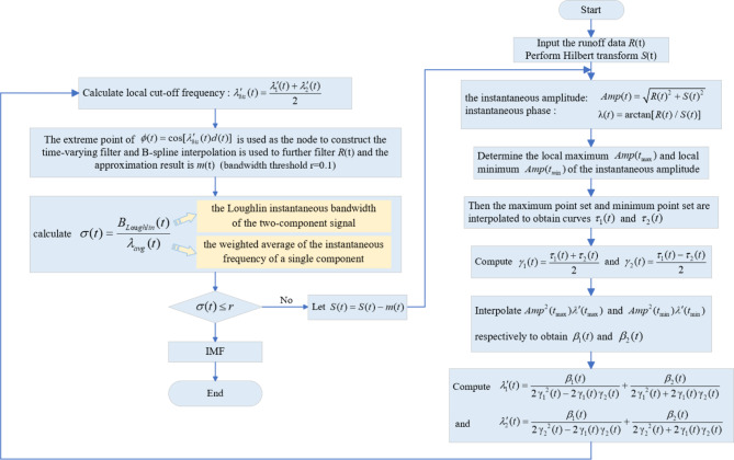
The TVFEMD employs a nonuniform B-spline approximation as a time-varying filter in the decomposition process. The local cutoff frequency of the TVFEMD is adaptively designed based on instantaneous amplitude and frequency information, and an approach to cutoff frequency rearrangement is introduced to address the intermittency problem. The calculation process of the TVFEMD method is illustrated in Fig. 1⁴³:

Fig. 1.

Implementation steps of the TVF-EMD.

Permutation entropy

The PE, proposed by Bandt & Pompe⁴⁴, is employed to characterize the complexity and self-similarity of a time series or a chaotic dynamical system. The method demonstrates remarkable ability to identify stochastic characteristics and fluctuations in non-linear time series. The methodology inherently has beneficial attributes for distinguishing signal randomness and isolating spurious elements. The process for calculating permutation entropy is as follows³⁷:

The phase space of the runoff series is first reconstructed to obtain the reconstruction matrix X:

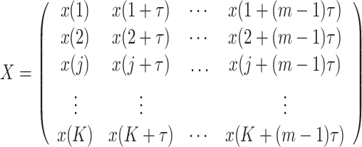2

where j = 1, 2, …, K; m represents the embedding dimension, τ signifies the delay time, and . Matrix X contains K rows of reconstructed components. Each reconstructed component is sequentially arranged in ascending order based on its values. As such, each row in the reconstructed matrix X can yield a sequence:

3

where g = 1, 2, …, k and k ≤ m!, because there are m! different mapping sequences within the m-dimensional phase space. Assuming the probability of occurrence for each mapping sequence is P₁, P₂, … P_k, the permutation entropy of a runoff sequence with k distinct mapping sequences can be defined as Eq. (4):

4

When , HP reaches its maximum value of ln(m! ). Normalize the value of HP as Eq. (5):

5

The magnitude of represents the complexity or randomness of the runoff sequence. A larger value of indicates increased randomness within the runoff sequence correlating with a higher potential for abrupt events, while sequence with reduced randomness suggest a lower likelihood of significant change.

Temporal convolutional network

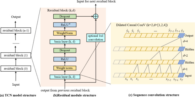
The fixed-length receptive field in CNN might not capture long-term dependencies in data sequences, thereby limiting accuracy in predictions. Responding to this, Bai et al.²⁴ introduced an advanced CNN model: TCN. TCN is a novel approach to processing time series data, comprising crucial components such as causal convolution, dilated convolution, and residual connections. An illustration of TCN’s fundamental building blocks is presented in Fig. 2.

Fig. 2.

Architectural elements in a TCN.

Causal convolution

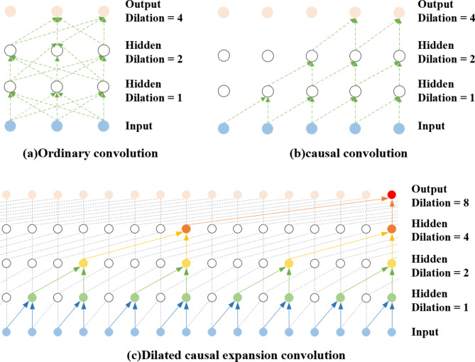
CNN is highly proficient in feature extraction but is rarely employed in time series prediction due to its structural defect - an inherent ‘information leakage’, as shown in Fig. 3-a, where the output of a current timestep is concatenated with elements from the future, which compromises predictive accuracy²³. TCN addresses this by employing a technique known as causal convolution. This technique circumvents the issue of information leakage, rendering it suitable for time series forecasting. Additionally, TCN employs a convolution stride of 1 and employs zero-padding that matches the kernel size minus one. This paradigm enables TCN to preserve the dimensionality of the input in the output as it processes temporal data through a fully convolutional network, thereby enhancing the model’s performance and precision. Figure 3-b illustrates the enhanced architecture of causal convolution⁴⁵.

Fig. 3.

Structures of three different convolution.

Dilation convolution

Observing Fig. 3b, it becomes evident that, while causal convolutions adhere to the principles of temporal continuity, they have a limited coverage of past input information, which can result in the loss of many historical data points. To mitigate this issue, TCN introduces a dilation rate d. This is achieved by inserting spaces or ‘gaps’ between the elements of the convolution kernel⁴⁶. Figure 3- illustrates the concept. The mathematical model for the dilated convolution, which is unfolded on a sequence element X of the one-dimensional sequence input and the filter , is presented as Eq. (6):

6

where s corresponds to the element of the one-dimensional input sequence, signifies the filter of size k, d represents the dilation rate, and is the index of the time step that has regressed⁴⁷.

Residual connections

During the integration of causal and dilated convolutions to extend the receptive field of TCN, there is an increase in the number of layers in the network. This can potentially lead to problems related to the vanishing or exploding of gradients. To address these challenges, residual connections are employed to maintain the stability and efficiency of the training. The fundamental concept of a residual connection is that it enables a certain layer within the network to directly access information from preceding layers. Through skip or shortcut connections, inputs can be transmitted to the next layer and reappear after skipping certain layers. This method effectively solves the problems of gradient disappearance and explosion during backpropagation by allowing gradients to be ‘short-circuited’ through these connections, thereby preserving gradient stability. The residual structure design is depicted in Fig. 2-c, featuring several residual units that directly map deep-level temporal sequence characteristics, thereby enhancing the learning capability of the TCN⁴⁷.

Proposed hybrid modeling

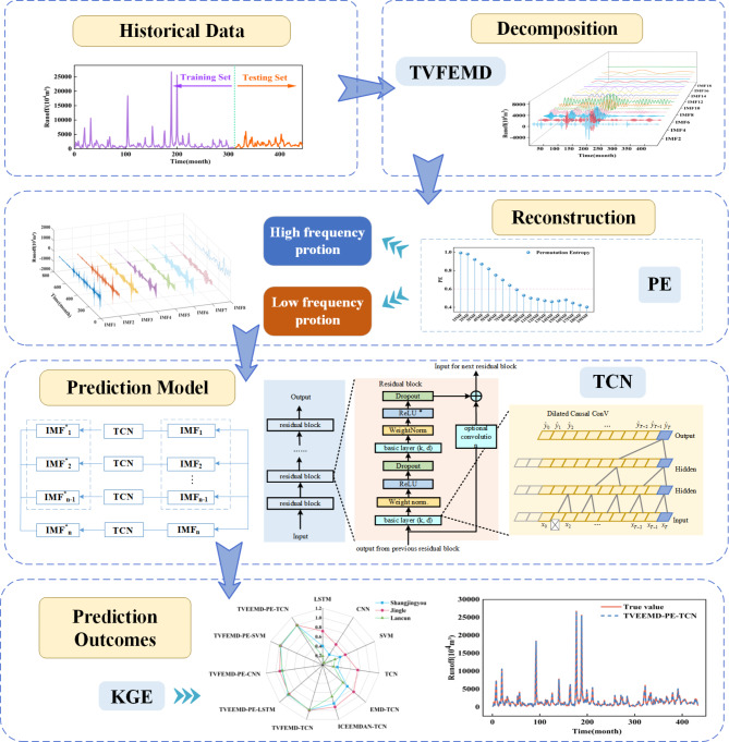
In this study, we initially applied the ERS unit root test to the monthly runoff sequence, revealing its non-stationary nature. Subsequently, we employed the TVFEMD technique to decompose the non-stationary runoff series into multiple IMFs. Next, the IMFs were classified into high-frequency and low-frequency components based on their permutation entropy values. This was followed by clustering the low-frequency components. We then utilized the TCN model to forecast the subsequences of the runoff sequence. The forecasts for both high-frequency and low-frequency components were combined to yield the definitive runoff prediction. The TVFEMD-PE-TCN composite model effectively combines the strengths of its constituents, providing a more reliable and accurate monthly runoff prediction. In the final assessment, the model’s applicability was evaluated using performance metrics, and the integrated TVFEMD-PE-TCN model is illustrated in Fig. 4.

Fig. 4.

Flow chart of the hybrid TVFEMD-PE-TCN model.

Evaluation indicators

To assess the effectiveness of the new runoff forecasting method and compare the proposed model with other benchmark models, five evaluation metrics were utilized. These include the root mean square error (RMSE), coefficient of determination (R²), mean absolute error (MAE), qualification rate (QR), Nash-Sutcliffe efficiency coefficient (NSE), and Kling-Gupta efficiency coefficient (KGE). MAE and RMSE assess the magnitude of errors between predicted and actual values, while NSE and R² gauge the fitting effect of hydrological forecast values against actual data. QR serves as an index for evaluating the predictive accuracy of hydrological models. KGE takes into account multiple aspects of model performance, including bias, variability, and correlation, offering a more comprehensive assessment than other measures. As KGE, NSE, and R² approach 1, and RMSE and MAE lower, QR approaches 100%, indicating a reduction in model prediction errors and an increase in predictive precision, thereby providing more reliable and accurate solutions for practical applications^48–50. The calculation formulas are presented in Eqs. (7)-(12) as follows:

7

8

9

10

11

12

where, represents the original runoff sequence, is the mean of the original runoff sequence, denotes the predicted runoff sequence values, is the mean of the predicted runoff sequence values, n is the count of runoff sequences, k represents the number of qualified predictions, and predictions are considered satisfactory if the absolute value of the relative prediction error is less than 20%. l is the length of the runoff sequence in the verification period. is variability bias,is the mean bias, r is the correlation coefficient, and σ and μ represents the standard deviation and the mean of the observed values, respectively.

Case study

Study areas

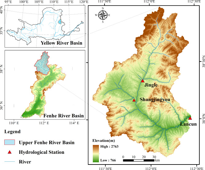
The Fenhe River spans a total length of 716 km(35°20′-38°56′N, 110°30′ − 113°32′ E), ranking as the second-largest tributary of the Yellow River. The Fenhe River basin, covering an area of approximately 3.9 × 10⁴ km². The topography diminishes from south to north, with a relatively large undulation and varied terrain. In recent years, a combination of natural factors and increased human water use has led to a significant reduction in the measured annual runoff of the Fenhe River basin⁵¹. This has severely impacted the economic and social development within the basin and exacerbated the degradation of the ecological environment. The upper reaches of the Fenhe River, as a crucial water source area of the river, also serve as an important surface water source for the capital city, Taiyuan, in Shanxi province⁴⁹. Against the backdrop of ecological construction, enhancing the accuracy of runoff forecasting is of critical importance for adaptive water resource management. To explore the model robustness to different runoff sizes at different hydrological stations, we selected three hydrological stations in the upper Fenhe River basin for our study: Shangjingyou, Lancun, and Jingle, as illustrated in Fig. 5. Three stations with significantly different catchment areas and runoff conditions were selected for model performance evaluation. Specifically, the Jingle station is located in the upper reaches of the Fenhe River basin, where the runoff variations are influenced by measures such as soil and water conservation. The Shangjingyou station is situated on a tributary of the Fenhe River basin, characterized by a relatively small runoff volume, which is subject to influences from various topographic and geomorphological features. In comparison, the Lanchun station has the largest drainage area under its control, with its runoff being significantly affected by large-scale human activities. Considering the uneven distribution of hydrological stations in the basin and the comprehensive coverage of the impact of human activities on runoff changes upstream, a further analysis of the model’s applicability under different flow and runoff conditions within the same basin is conducted⁵². By establishing an accurate runoff prediction model, scientific management strategies can be provided for local governments, which will have a profound impact on economic development and people’s production and life.

Fig. 5.

Geographical overview of the study area. The map was generated using ArcMap 10.8 (https://www.esri.com/en-us/arcgis/products/arcgis-desktop/overview).

Data source

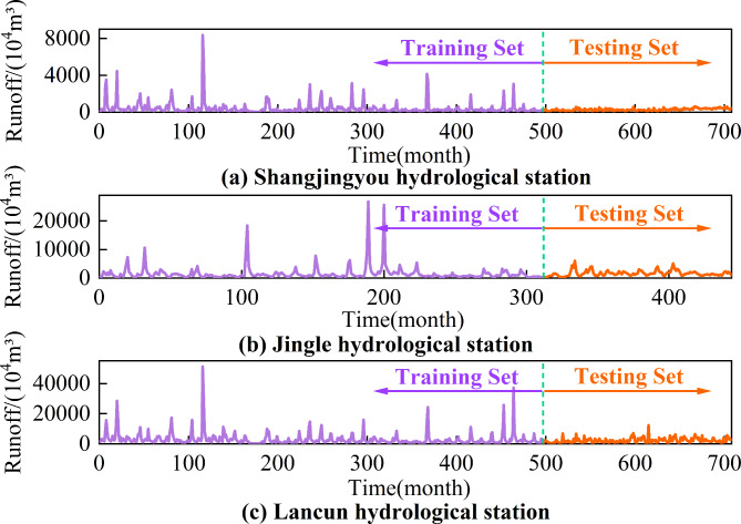
In this study, 70% of the data is set aside for training, while the remaining 30% is designated as the test set for each dataset. This allocation is intended to prevent any ‘leakage’ of calibration data during the validation phase. It is designed to guarantee that the performance of model on the test set is robust and not unduly influenced by random variations⁵³. This step is essential to overcome any biases in the model results that might arise from the use of future data. The original runoff sequence is illustrated in Fig. 6.

Fig. 6.

Hydrological station data set image.

To enhance the convergence speed of the model, normalization was applied to all the data, ensuring that the range of all values is scaled between 0 and 1. The description of this expression is as follows:

where and represent the normalized result and sample data, respectively; and are the maximum and minimum values in the sample, respectively.

Runoff characteristics analysis

Descriptive statistical analysis was conducted on the monthly runoff datasets from the three hydrological stations. The results of this analysis are presented in Table 1. As demonstrated in Table 1, the monthly runoff at the three hydrologic stations exhibited significant variation, with an uneven distribution throughout the year, substantial variation, and the presence of numerous extreme values.

Table 1.

Characteristics of monthly runoff data of three hydrological stations.

	Min (104 m3/s)	Max (104m3/s)	Mean (104m3/s)	Std (104m3/s)	Skewness	Kurtosis
Shangjingyou	28	8379	383.63	575.68	7.22	72.37
Jingle	148	26,728	1596.77	2243.67	7.42	71.56
Lancun	6	51,252	2782.06	3785.61	6.27	57.50

The monthly runoff datasets from the three hydrological stations were tested the stationarity, and the results of the ERS unit root test are shown in Table 2. It can be seen from Table 2 that the ERS unit root test statistics P for the three hydrological stations all exceeded the critical values at the 1% significance level. Therefore, we cannot reject the null hypothesis of the presence of a unit root, indicating that the runoff series for the three hydrological stations possess strong characteristics of non-stationarity.

Table 2.

ERS Unit Root Test results for three hydrological stations data set.

Data Set	P-Statistic	Stationary?
Shangjingyou	17.03	Nonstationary
Jingle	5.7	Nonstationary
Lancun	38.14	Nonstationary
5% Critical Value	4.22

Determining input variables and model parameters

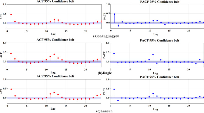
The autoregressive coefficient method to ascertain the lag time, which serves as an input variable for the model. The Autocorrelation Function (ACF) and Partial Autocorrelation Function (PACF) are utilized to select the optimal lag time, thereby defining the input step length of the model.

Figure 7 presents the ACF and PACF plots for the three stations. The plots indicate that the ACF estimates for each station peaked at the 12th delay time point, while the PACF estimates stabilizing within the 95% confidence interval beyond the 12th lag. Consequently, the input data for the runoff prediction model consist of historical runoff data covering the previous 12 months.

Fig. 7.

ACF and PACF diagrams of initial runoff series.

This research involved multiple experiments with different combinations of model parameters at the Shangjingyou hydrological station. By comparing the prediction loss functions and the predictive performance on the test set, the most optimal model construction strategy was identified. Table 3 presents the optimal sets of parameters for constructing each model.

Table 3.

Parameter settings of the models.

Model	Parameter	Value
TVFEMD	B-spline order n	50
	Bandwidth threshold ζ	0.25
TCN	Kernel size	8
	Residual block	2
	Filters	64
	Learning rate	0.001
	Batch size	128
	Epochs	500
	Activation function	ReLU
	Optimizer	Adam
	Loss function	RMSE
LSTM	Hidden layers	2
	Hidden size	256
	Learning rate	0.001
	Epochs	500
	Optimizer	Adam
	Loss function	RMSE
CNN	Convolutional layers	2
	Kernel size	3 × 1
	Batch size	128
	Epochs	500
	Activation function	ReLU
	Optimizer	Adam
	Loss function	RMSE
SVM	c	4.0
	Gamma	0.8
PE	Embedded dimension	5

Results

Decomposition and clustering results

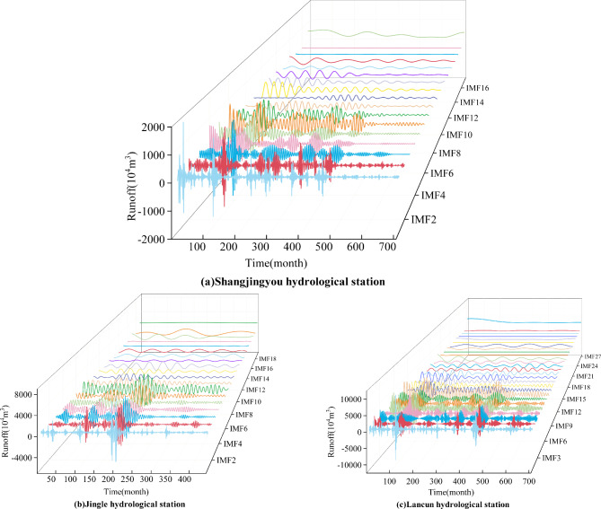
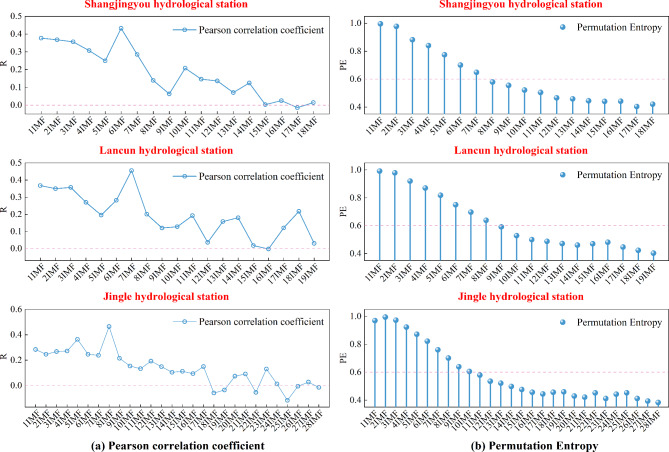
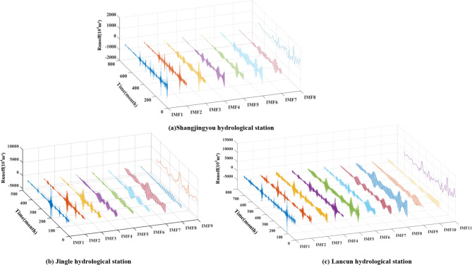
Figure 8 presents the results of the TVFEMD for the monthly runoff data sets measured at three hydrological stations. The original dataset is decomposed into IMFs with different frequencies, thereby enhancing the potential for increased prediction accuracy. However, the presence of a larger number of IMFs, such as the 27 contained in the Lancun station dataset, adds significant complexity and higher computational cost to the runoff forecasting model. Moreover, the low-frequency components often demonstrate a weaker correlation, and even negative correlation, with the original runoff sequences (as shown in Fig. 9a). Consequently, we introduced PE to ascertain the complexity of each IMF, with the results shown in Fig. 9b. The distinction between high-frequency and low-frequency components is made by defining the boundary according to the parts with bigger changes in each IMF. Specifically, the sub-sequence that immediately follows a pair of IMFs is identified as the concluding segment of the high-frequency component, while the commencement of the low-frequency component is derived from the subsequent sub-sequence. Our methodological approach enables a more precise bifurcation of signal into high-frequency and low-frequency components, which is a pivotal step in a multitude of signal processing applications⁵⁴. Resultant clustering of low-frequency IMFs, post the demarcation of high-frequency components as those exceeding 0.6 and low-frequency elements as those beneath 0.6¹⁷, are delineated in Fig. 10. The prediction accuracy is improved by clustering the low-frequency components, which in turn reduces the accumulation of prediction errors by the less correlated components.

Fig. 8.

TVFEMD results of monthly runoff at each hydrological station.

Fig. 9.

Pearson correlation coefficient and PE results of monthly runoff at each hydrological station.

Fig. 10.

Clustering results of monthly runoff for each hydrological station.

Model development and prediction results

The objective of this study is to validate the efficacy of our proposed TVFEMD-PE-TCN model from four perspectives. Firstly, the predictive prowess of TCN model is gauged against three single models: LSTM, CNN and SVM. This measures the individual competence of TCN. The second involves comparing the performance of EMD, ICEEMDAN, and TVFEMD, applied to non-stationary runoff data from three hydrological stations. This affirms the effectiveness of using the TVFEMD technique for decomposing the original runoff series into IMFs. The third step amalgamates the four base models with the TVFEMD and PE to create hybrid forecasting models. This procedure underscores the competitive edge of our proposed TVFEMD-PE-TCN model. Lastly, to highlight the superiority of our model, we contrasted the forecast accuracy and time consumption of the hybrid model before and after the introduction of PE to cluster the low-frequency sub models. This final analysis affirms the feasibility of applying PE for clustering in low-frequency sub-models. A comprehensive assessment of the forecasting outcomes, including four evaluation metrics, is consolidated and presented in Table 4.

Table 4.

Comparative evaluation of runoff prediction outcome metrics among different models.

Sites	Models	Training set				Testing set
		RMSE	MAE	NSE	R2	RMSE	MAE	NSE	R2
Shangjingyou	LSTM	546.87	229.18	0.30	0.56	114.85	93.76	0.11	0.52
	CNN	407.09	195.62	0.61	0.79	280.84	196.94	-4.34	0.34
	SVM	565.55	194.56	0.26	0.53	97.27	72.98	0.36	0.65
	TCN	566.91	252.97	0.25	0.50	116.69	98.52	0.08	0.59
	EMD-TCN	493.82	283.04	0.43	0.70	81.42	65.17	0.55	0.75
	ICEEMDAN-TCN	372.76	191.38	0.68	0.83	50.90	37.97	0.82	0.92
	TVFEMD-TCN	47.30	32.19	0.995	0.997	10.20	8.18	0.993	0.997
	TVEEMD-PE-LSTM	165.25	99.03	0.94	0.97	25.57	20.10	0.96	0.98
	TVFEMD-PE-CNN	54.28	40.07	0.993	0.997	51.29	42.11	0.82	0.96
	TVFEMD-PE-SVM	58.13	39.96	0.992	0.996	13.67	11.00	0.987	0.995
	TVEEMD-PE-TCN	47.25	32.13	0.995	0.997	9.20	7.42	0.994	0.997
Jinle	LSTM	1995.80	782.38	0.41	0.65	716.46	472.85	0.44	0.73
	CNN	977.30	536.02	0.86	0.93	902.91	609.34	0.11	0.55
	SVM	1975.71	625.65	0.43	0.75	713.10	443.55	0.44	0.75
	TCN	2150.55	885.02	0.32	0.57	696.50	453.51	0.47	0.70
	EMD-TCN	1983.56	1098.12	0.42	0.72	484.05	346.38	0.74	0.88
	ICEEMDAN-TCN	1602.21	840.07	0.62	0.82	348.23	234.16	0.87	0.93
	TVFEMD-TCN	125.83	93.04	0.998	0.999	52.68	41.74	0.997	0.998
	TVEEMD-PE-LSTM	586.53	360.73	0.95	0.98	220.57	173.73	0.95	0.98
	TVFEMD-PE-CNN	204.22	152.24	0.994	0.997	253.10	200.46	0.93	0.98
	TVFEMD-PE-SVM	167.38	120.00	0.996	0.998	83.31	66.96	0.992	0.997
	TVEEMD-PE-TCN	125.54	92.24	0.998	0.999	44.33	33.74	0.998	0.999
Lancun	LSTM	3456.37	1504.57	0.36	0.61	1659.05	1109.75	-0.03	0.28
	CNN	2553.23	1301.26	0.65	0.81	2671.06	1843.21	-1.68	0.29
	SVM	3422.30	1279.24	0.38	0.65	1602.96	991.72	0.04	0.37
	TCN	3578.32	1664.83	0.32	0.56	1572.67	1108.58	0.07	0.37
	EMD-TCN	1640.82	1159.39	0.86	0.93	1583.12	1198.15	0.06	0.64
	ICEEMDAN-TCN	1367.04	931.77	0.90	0.95	1128.44	853.01	0.52	0.77
	TVFEMD-TCN	167.71	119.05	1.00	1.00	127.61	105.75	0.994	0.997
	TVEEMD-PE-LSTM	834.02	535.54	0.96	0.98	368.99	284.39	0.95	0.98
	TVFEMD-PE-CNN	313.02	236.23	0.99	0.998	478.89	379.60	0.91	0.98
	TVFEMD-PE-SVM	260.27	187.49	0.996	0.998	138.42	108.10	0.993	0.996
	TVEEMD-PE-TCN	169.20	120.58	0.998	0.999	106.68	80.12	0.996	0.998

Discussion

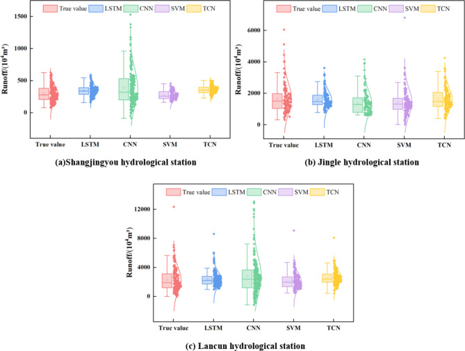
The box normal chart for each single model on each hydrological station testing set is shown in Fig. 11 for a direct assessment of model accuracy. Compared with other single models, the TCN model performs stably and superiorly in runoff prediction for test set at the three hydrological stations, especially at the Lancun hydrological station. LSTM encounters issues like gradient vanishing or exploding when dealing with long sequence data. SVMs over-adapt to the training data, prone to overfitting due to the influence of runoff peaks. CNNs also exhibit strong dependence on the training data, leading to poor generalization capabilities. This renders them less effective in modeling long-term dependencies, thereby limiting their predictive accuracy. In contrast, the TCN model architecture, constructed with causal dilated convolutions, combines skip connections and dilated convolutions to mitigate the problems of gradient vanishing and exploding, while aiding in the capture of long-term dependencies, thus achieving good long-term memory on sequential data. Furthermore, by reducing the number of parameters and the complexity of the model, it effectively alleviates overfitting and enhances generalization. This justifies that employing the TCN model for predicting runoff sequences is a pragmatic and feasible approach. Moreover, it is evident that prediction of these single models is markedly poor, in particular peak runoff. Hence, data preprocessing techniques are critical to enhance the predictive models.

Fig. 11.

Single model prediction results on the testing set for each hydrological station.

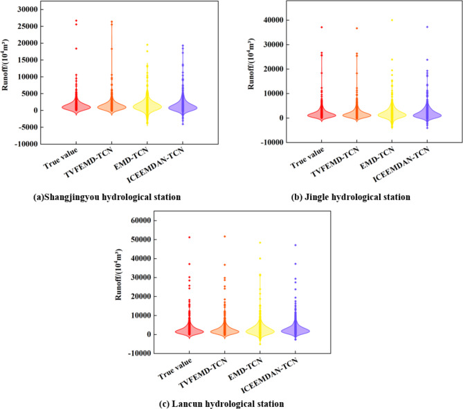
According to the evaluative metrics delineated in Table 4, the TCN ensemble model coupled with decomposition methods has demonstrated improved precision over the single TCN model in runoff forecasting. Out of the three signal decomposition preprocessing techniques, the TVFEMD-TCN has emerged with superior predictive performance, suggesting that the TVFEMD is more effective at mitigating spectral mode leakage and edge effects than EMD and ICEEMDAN. This is evidenced by some instances in the Shangjingyou hydrological station, where the TVFEMD-TCN model has achieved a reduction of 87.47% and 79.96% in RMSE respectively, compared with the corresponding EMD-TCN and ICEEMDAN-TCN models. The MAE has been reduced by 87.45% and 78.46%, the NSE has increased by 80.13% and 20.41%, and the R² has climbed by 32.60% and 8.87%. At the Jingle hydrological station, in comparison to the above signal decomposition techniques, the TVFEMD-TCN model has decreased RMSE by 89.12% and 84.87%. Furthermore, the MAE has been lowered by 87.95% and 82.18%. The NSE has seen an improvement of 34.03% and 14.93%, and the R² has climbed by 13.16% and 6.89%. At the Lancun hydrological station, compared to the combination models of the aforementioned decomposition methods, the TVFEMD-TCN model has reduced RMSE and MAE by 63.94-91.94% and 59.71-91.17% respectively. The NSE and R² have increased by 0.08–0.94 and 3.09-58.43%. The TVFEMD-TCN model has achieved NSE of up to 0.99 during both training and validation periods across the three hydrological stations. This is mainly due to the ability of TVFEMD to lessen the prediction difficulty of high-frequency components and effectively present the characteristics of the original runoff sequence. As shown in Fig. 11, which features violin plots of the runoff prediction results from different decomposition methods coupled with TCN at each hydrological station, the model based on TVFEMD decomposition achieves the best prediction performance out of all stations. This suggests that TVFEMD has an excellent decomposition capability for nonstationary runoff sequence data (Fig. 12).

Fig. 12.

Prediction results of different combination models on the testing set for each hydrological station.

Worth mentioning is that the models based on the ‘Decomposition-Prediction-Integration’ framework have shown significant improvements in terms of simulation fit compared to the single models, as evident in Fig. 13. At the Shangjingyou hydrological station, the coupled models of TVFEMD-PE-LSTM, TVFEMD-PE-CNN, TVFEMD-PE-SVM, and TVFEMD-PE-TCN have seen a reduction in RMSE of 77.73%, 81.74%, 85.94% and 92.11%, respectively during the testing set compared to their corresponding single models. For the Jingle hydrological station, the same coupled models have achieved a reduction in RMSE of 69.21%, 71.97%, 88.32% and 93.64% respectively during the testing set when compared to their respective single models. At the Lan Cun hydrological station, the coupled models have decreased RMSE by 77.76%, 82.07%, 91.36%, and 93.22% respectively during the testing set compared to their matching single models. The substantial enhancements can be credited to the signal decomposition technology and PE clustering, which splits the original runoff sequence into several relatively smooth sub-models that are more manageable and facilitate the extraction of features for more accurate runoff forecasting.

Fig. 13.

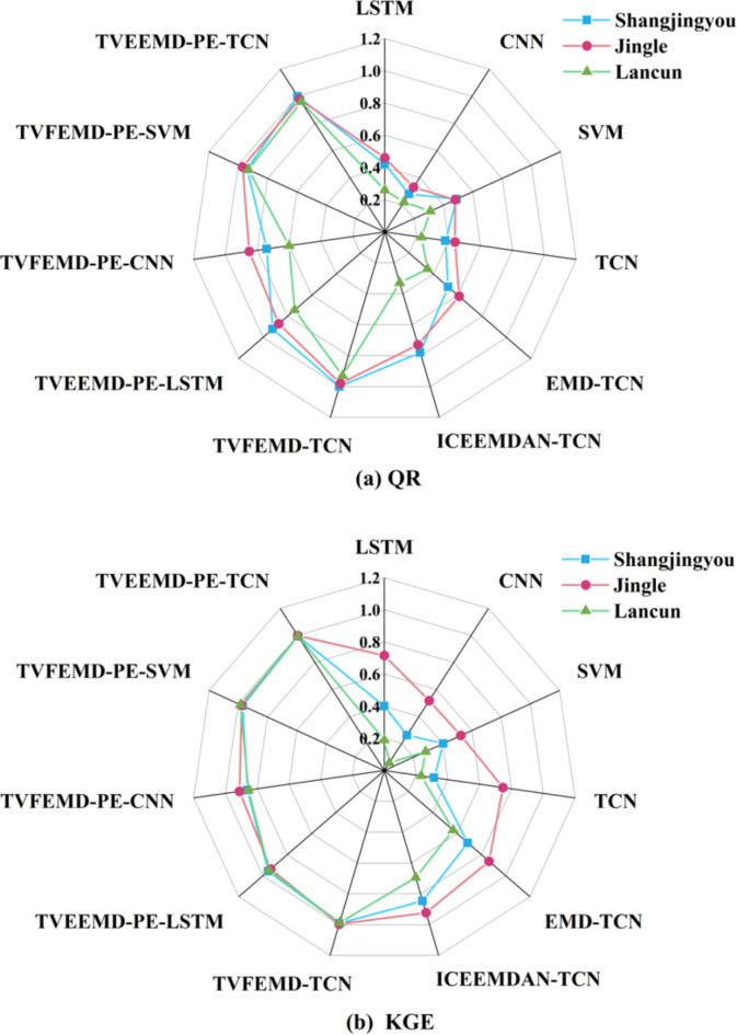
The QR and KEG of each model on the testing set of three hydrological stations.

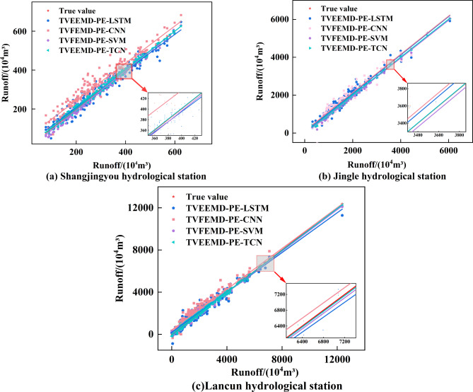
Figure 14 presents the regression images of each hybrid model on the testing set of the three hydrological stations. Figure 14 shows the TVFEMD-PE-TCN model has the highest R², which all achieve 0.99, indicating that TVFEMD-PE-TCN performs the best in terms of fitting accuracy among all hybrid models. Furthermore, at the Shangjingyou hydrological station, the TVFEMD-PE-TCN model has declined RMSE by 64.01%, 82.05% and 32.67% respectively during the testing set compared to the TVFEMD-PE-LSTM, TVFEMD-PE-CNN and TVFEMD-PE-SVM models. Regarding the Jingle hydrological station, the RMSE of the TVFEMD-PE-TCN model has been decreased by 79.90%, 82.48% and 46.79% respectively compared to the previously mentioned models. Taking the Lancun hydrological station as an example, the RMSE on the testing set for the TVFEMD-PE-TCN model is 71.09%, 77.72%, and 222.93% lower than other hybrid models. The exceptionally high predictive capability of the TVFEMD-PE-TCN model for runoff forecasting can be attributed to the ability of TCN to facilitate cross-layer information transfer through residual connections. This ensures that shallow-layer information is seamlessly relayed to deeper layers, enhancing the efficiency of the backpropagation process. Therefore, predicting with the TCN not only eliminates residual noise in the data that could not be removed by preliminary decomposition techniques but also further exploits the temporal characteristics of the subsequence data derived from TVFEMD decomposition and clustering, thereby offering a more accurate and stable fit for runoff.

Fig. 14.

The regression images of each combined model on the testing set of three hydrological stations.

In addition, Fig. 13 shows the QR and KGE values for each model.The closer the NSE and KGE values are to 1, this means that the model predictions are closer to the actual observations. As can be seen from the Fig. 13, the symbols indicating the TVFEMD-PE-TCN model are closer to 1, which means that its prediction ability is excellent. This result proves that the model proposed in this study significantly reduces the anomalous fluctuations in the prediction results with low uncertainty.

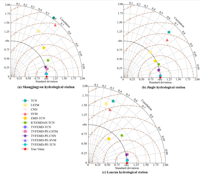
Figure 15 presents Taylor diagrams for the Shangjingyou, Jingle, and Lancun hydrological stations, providing a concise representation of multiple models’ statistical information and showcasing the results of three evaluation metrics in a single image. The Taylor diagram in this study employs three evaluation metrics: RMSE (normalized), NSE, and R². The horizontal and vertical axes represent NSE, R² is depicted by radial lines, and dashed lines signify RMSE. Different patterns signify different model behaviors, where the symbol representing a model is closer to the center of the plot if its predictions are closer to the actual values. From Fig. 14, it is evident that the TVFEMD-PE-TCN model is closer to the actual values compared to other predictive models, referencing the best forecast performance and the highest predictive accuracy.

Fig. 15.

Taylor diagrams for the testing set of 18 forecast models at various hydrological stations.

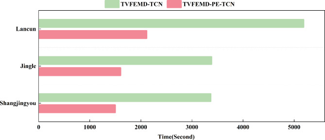
Figure 16 provides a comparative analysis of prediction durations for the TVFEMD-TCN and TVFEMD-PE-TCN composite models. Referring to Table 4, it is observed that the application of the TVFEMD-PE-TCN model has resulted in a notable decrease in RMSE by 9.75%, 15.85%, and 16.40% at the three hydrological stations compared to the TVFEMD-TCN model. This corroborates the efficacy of utilizing PE to assess the complexity of each constituent part of the IMF. Furthermore, when juxtaposed with the TVFEMD-TCN model, the prediction time and computational costs of the TVFEMD-PE-TCN model are significantly reduced across the three hydrological stations. These findings further substantiate the pragmatic utility of employing PE to evaluate the complexity of every component within the IMF. Consequently, it is deemed feasible to utilize PE in assessing the complexity of each variable IMF component, thereby clustering relatively smooth low-frequency sequences.

Fig. 16.

Modeling time of runoff sequences for different models at various hydrological stations.

Table 5 presents the prediction values and errors of runoff extremes at the three hydrological stations during the test set for each model. As Table 5 illustrates, the TVFEMD-PE-TCN model significantly reduced the prediction errors for extreme values compared to other models. Specifically, the extreme value errors at the three stations for the TVFEMD-PE-TCN model were reduced by 74.96%, 22.65%, and 20.81%, respectively, compared to the TVFEMD-TCN model. This indicates that, following clustering with the PE method, the predicted extreme values are closer to the actual values, and the performance of model in predicting extremes has been improved over the original model. Overall, the proposed model not only enhances the overall prediction accuracy but also shows a notable improvement in local extreme value prediction.

Table 5.

The error of the extreme values of the test set for three stations.

	Jinle (104m3)		Shangjingyou (104m3)		Lancun (104m3)
	Runoff	Error	Runoff	Error	Runoff	Error
Peak runoff	6049		625		12,362
TCN	2005	-4044	503	-122	1964	-10,398
LSTM	2089	-3960	536	-89	1720	-10,642
CNN	1292	-4757	1170	545	2174	-10,188
SVM	1973	-4076	387	-238	1530	-10,832
EMD-TCN	4989	-1060	553	-72	15,437	3075
ICEEMDAN-TCN	4917	-1132	624	-1	9019	-3343
TVFEMD-TCN	6010	-39	627	2	12,280	-82
TVEEMD-PE-LSTM	5910	-139	647	22	11,280	-1082
TVFEMD-PE-CNN	6074	25	682	57	12,136	-226
TVFEMD-PE-SVM	6022	-27	629	4	12,114	-248
TVEEMD-PE-TCN	6039	-10	626	1	12,297	-65

Tables 1 and 2 indicates that the P-values from the ERS test and the statistical characteristics of runoff at three hydrological stations are distinct. This indicates that the selected stations have significantly different runoff variability characteristics. The significant changes in the runoff pattern make these stations an effective case for evaluating the generalization and adaptability of the model. The statistical characteristics of the runoff unveil significant changes, which may be attributed to the combined effects of climate, topography, soil types, and anthropogenic interventions. Despite the challenges posed by the diversity and complexity, the developed model showed excellent adaptability to the different runoff characteristics at three stations and excellent predictive performance. This achievement is primarily attributed to the model’s ability to learn the characteristics of various input data, effectively representing the hydrological properties of each station.

Conclusion

Accurate runoff prediction is essential for various practical applications, including water resource planning and flood forecasting. This paper introduces a novel TVFEMD-PE-TCN hybrid model to forecast monthly runoff at three hydrological stations. A comparison of predictive accuracy among different models led to the following conclusions:

1. The TVFEMD technique significantly enhances runoff prediction. Single neural network models often struggle with non-stationary data due to their inherent limitations in runoff prediction. The integration of TVFEMD improves model reliability and suitability. Compared to other decomposition techniques such as ICEEMDAN, the TVFEMD method, combined with TCN, yields the best predictive results, especially with high-frequency IMF signals. TVFEMD aids in mapping non-stationary runoff sequences into IMFs that facilitate the capture and extraction of data features. This approach enhances the comprehensiveness and sufficiency of time-series decomposition, reducing the interference of stochastic elements on deterministic ones.

2. The application of PE on TVFEMD decomposed sub-models enables a complexity evaluation and distinction between high and low-frequency components. Clustering is performed on low-frequency components, thereby generating new sub-components for forecasting. This not only significantly enhances model predictive accuracy but also conserves computational cost by substantially reducing the redundancy of sub-model information, obtaining improved practicality and prediction efficiency.

3. Compared to other hybrid models, the TVFEMD-PE-TCN model has achieved NSE and KGE values of 0.99 at all three hydrological stations, with the QR exceeding 96%. Notably, at the Shangjingyou station, the QR is 100%. TCN demonstrates more effective extraction from the features of sub-segments decomposed by TVFEMD. Therefore, this model lays a dependable method for monthly runoff time-series forecasting.

4. This study presents a composite prediction method that combines TVFEMD signal processing techniques, PE, and TCN to form a runoff prediction model, demonstrating higher prediction accuracy. It is an efficient and practical forecasting method, offering valuable support for decision making in water resources management within drainage basins.

Future studies could focus on integrating basin climatic attributes such as rainfall, evaporation, temperature, among others, and anthropogenic factors like land-use changes, geological conditions, to further refine the model and elevate its interpretability.

Author contributions

All authors contributed to the study conception and design. H.W.: Conceptualization, Methodology, Model development, Manuscript writing, and Analysis of results. X.Z.: Validation, Project administration, Resources, Supervision, Funding acquisition. Q.G.: Interpretation. Model development, Data curation. X.W.: Model development, Data collection.

Funding

This research is financially supported by the National Natural Science Foundation of China (Nos. 5227902), Special Fund for Science and Technology Innovation Teams of Shanxi Province (No. 202204051002027).

Data availability

The data used in this study are confidential and not publicly available. For access to the data or any related materials, please contact the corresponding author.

Declarations

Competing interests

The authors declare no competing interests.

References

- 1.Min, X., Hao, B., Sheng, Y., Huang, Y. & Qin, J. Transfer performance of gated recurrent unit model for runoff prediction based on the comprehensive spatiotemporal similarity of catchments. J. Environ. Manage.330, 117182 (2023). [DOI] [PubMed] [Google Scholar]
- 2.Guo, T. L. et al. A novel time-varying stepwise decomposition ensemble framework for forecasting nonstationary and nonlinear streamflow. J. Hydrol.617, 128836 (2023). [Google Scholar]
- 3.Yu, Q., Jiang, L., Wang, Y. & Liu, J. Enhancing streamflow simulation using hybridized machine learning models in a semi-arid basin of the Chinese loess Plateau. J. Hydrol.617, 129115 (2023). [Google Scholar]
- 4.Xu, D. M. et al. A new hybrid model for monthly runoff prediction using ELMAN neural network based on decomposition-integration structure with local error correction method. Expert Syst. Appl.238, 121719 (2024). [Google Scholar]
- 5.Zhang, X., Liu, F., Yin, Q., Wang, X. & Qi, Y. Daily runoff prediction during flood seasons based on the VMD-HHO-KELM model. Water Sci. Technol.88 (2), 468–485 (2023). [DOI] [PubMed] [Google Scholar]
- 6.Abbasi, M., Farokhnia, A., Bahreinimotlagh, M. & Roozbahani, R. A hybrid of Random Forest and Deep Auto-Encoder with support vector regression methods for accuracy improvement and uncertainty reduction of long-term streamflow prediction. J. Hydrol.597, 125717 (2021). [Google Scholar]
- 7.Guo, S., Wen, Y., Zhang, X. & Chen, H. Monthly runoff prediction using the VMD-LSTM-Transformer hybrid model: a case study of the Miyun Reservoir in Beijing. J. Water Clim. Change. 14 (9), 3221–3236 (2023). [Google Scholar]
- 8.Ahmed, A. M. et al. Deep learning hybrid model with Boruta-Random Forest optimiser algorithm for streamflow forecasting with climate mode indices, rainfall, and periodicity. J. Hydrol.599, 126350 (2021). [Google Scholar]
- 9.Wu, J., Wang, Z., Hu, Y., Tao, S. & Dong, J. Runoff forecasting using convolutional neural networks and optimized bi-directional long short-term memory. Water Resour. Manage.37 (2), 937–953 (2023). [Google Scholar]
- 10.Yao, Z., Wang, Z., Wang, D., Wu, J. & Chen, L. An ensemble CNN-LSTM and GRU adaptive weighting model based improved sparrow search algorithm for predicting runoff using historical meteorological and runoff data as input. J. Hydrol.625, 129977 (2023). [Google Scholar]
- 11.Feng, Z. K. et al. Monthly runoff time series prediction by variational mode decomposition and support vector machine based on quantum-behaved particle swarm optimization. J. Hydrol.583, 124627 (2020). [Google Scholar]
- 12.Xu, D. M., Li, Z. & Wang, W. C. An ensemble model for monthly runoff prediction using least squares support vector machine based on variational modal decomposition with dung beetle optimization algorithm and error correction strategy. J. Hydrol.629, 130558 (2024). [Google Scholar]
- 13.AlDahoul, N. et al. Streamflow classification by employing various machine learning models for peninsular Malaysia. Sci. Rep.13 (1), 14574 (2023). [DOI] [PMC free article] [PubMed] [Google Scholar]
- 14.Meng, E. et al. A robust method for non-stationary streamflow prediction based on improved EMD-SVM model. J. Hydrol.568, 462–478 (2019). [Google Scholar]
- 15.Meng, E. et al. A hybrid VMD-SVM model for practical streamflow prediction using an innovative input selection framework. Water Resour. Manage.35, 1321–1337 (2021). [Google Scholar]
- 16.He, C., Chen, F., Long, A., Qian, Y. & Tang, H. Improving the precision of monthly runoff prediction using the combined non-stationary methods in an oasis irrigation area. Agric. Water Manag. 279, 108161 (2023). [Google Scholar]
- 17.Wu, J. et al. Robust runoff prediction with explainable artificial intelligence and meteorological variables from deep learning ensemble model. Water Resour. Res.59 (9), e2023WR035676 (2023). [Google Scholar]
- 18.Wunsch, A., Liesch, T. & Broda, S. Groundwater level forecasting with artificial neural networks: a comparison of long short-term memory (LSTM), convolutional neural networks (CNNs), and non-linear autoregressive networks with exogenous input (NARX). Hydrol. Earth Syst. Sci.25 (3), 1671–1687 (2021). [Google Scholar]
- 19.Swagatika, S., Paul, J. C., Sahoo, B. B., Gupta, S. K. & Singh, P. K. Improving the forecasting accuracy of monthly runoff time series of the Brahmani River in India using a hybrid deep learning model. Water Clim. Change. 15 (1), 139–156 (2024). [Google Scholar]
- 20.Xu, Y. et al. Improved convolutional neural network and its application in non-periodical runoff prediction. Water Resour. Manage.36 (15), 6149–6168 (2022). [Google Scholar]
- 21.Martinho, A. D., Hippert, H. S. & Goliatt, L. Short-term streamflow modeling using data-intelligence evolutionary machine learning models. Sci. Rep.13 (1), 13824 (2023). [DOI] [PMC free article] [PubMed] [Google Scholar]
- 22.Essam, Y. et al. Predicting streamflow in Peninsular Malaysia using support vector machine and deep learning algorithms. Sci. Rep.12 (1), 3883 (2022). [DOI] [PMC free article] [PubMed] [Google Scholar]
- 23.Dong, X., Sun, Y., Li, Y., Wang, X. & Pu, T. Spatio-temporal convolutional network based power forecasting of multiple wind farms. J. Mod. Power Syst. Clean. Energy. 10 (2), 388–398 (2021). [Google Scholar]
- 24.Bai, S., Kolter, J. Z. & Koltun, V. An empirical evaluation of generic convolutional and recurrent networks for sequence modeling. arXiv:1803.01271 (2018).
- 25.Zhang, C., Sheng, Z., Zhang, C. & Wen, S. Multi-lead-time short-term runoff forecasting based on ensemble attention temporal Convolutional Network. Expert Syst. Appl.243, 122935 (2024). [Google Scholar]
- 26.Xu, Y. et al. Application of temporal convolutional network for flood forecasting. Hydrol. Res.52 (6), 1455–1468 (2021). [Google Scholar]
- 27.Ng, K. W. et al. A review of hybrid deep learning applications for streamflow forecasting. J. Hydrol. 130141 (2023).
- 28.Wang, W. C. et al. Encoding and decoding monthly runoff prediction model based on deep temporal attention convolution and multimodal fusion. J. Hydrol. 643. DTTR, 131996 (2024). [Google Scholar]
- 29.Wang, W. C. et al. Evaluating the performance of several data preprocessing methods based on GRU in forecasting monthly runoff time series. Water Resour. Manage. 1–18 (2024).
- 30.Wang, T., Liu, T. & Lu, Y. A hybrid multi-step storm surge forecasting model using multiple feature selection, deep learning neural network and transfer learning. Soft Comput.27 (2), 935–952 (2023). [Google Scholar]
- 31.Yang, C., Jiang, Y., Liu, Y., Liu, S. & Liu, F. A novel model for runoff prediction based on the ICEEMDAN-NGO-LSTM coupling. Environ. Sci. Pollut Res.30 (34), 82179–82188 (2023). [DOI] [PubMed] [Google Scholar]
- 32.Yan, X., Chang, Y., Yang, Y. & Liu, X. Monthly runoff prediction using modified CEEMD-based weighted integrated model. Water Clim. Change. 12 (5), 1744–1760 (2021). [Google Scholar]
- 33.Song, C., Chen, X., Wu, P. & Jin, H. Combining time varying filtering based empirical mode decomposition and machine learning to predict precipitation from nonlinear series. J. Hydrol.603, 126914 (2021). [Google Scholar]
- 34.Zhang, C. et al. An evolutionary deep learning model based on TVFEMD, improved sine cosine algorithm, CNN and BiLSTM for wind speed prediction. Energy254, 124250 (2022). [Google Scholar]
- 35.Chen, S., Ren, M. & Sun, W. Combining two-stage decomposition based machine learning methods for annual runoff forecasting. J. Hydrol.603, 126945 (2021). [Google Scholar]
- 36.Wang, W. C. et al. An ensemble hybrid forecasting model for annual runoff based on sample entropy, secondary decomposition, and long short-term memory neural network. Water Resour. Manage.35, 4695–4726 (2021). [Google Scholar]
- 37.Zhang, X., Tuo, W. & Song, C. Application of MEEMD-ARIMA combining model for annual runoff prediction in the Lower Yellow River. Water Clim. Change. 11 (3), 865–876 (2020). [Google Scholar]
- 38.Zhang, Y., Yang, Z., Du, X. & Luo, X. A new method for denoising underwater acoustic signals based on EEMD, correlation coefficient, permutation entropy, and wavelet threshold denoising. J. Mar. Sci. Appl.23 (1), 222–237 (2024). [Google Scholar]
- 39.Ruiz, M. D. C., Guillamón, A. & Gabaldón, A. A new approach to measure volatility in energy markets. Entropy14 (1), 74–91 (2012). [Google Scholar]
- 40.Xu, D. M., Hong, Y. H., Wang, W. C., Li, Z. & Wang, J. A novel daily runoff forecasting model based on global features and enhanced local feature interpretation. J. Hydrol. 132227 (2024).
- 41.Elliott, G., Rothenberg, T. J. & Stock, J. H. Efficient tests for an autoregressive unit root. Econometrica64, 813–836 (1996). [Google Scholar]
- 42.Westerlund, J. A computationally convenient unit root test with covariates, conditional heteroskedasticity and efficient detrending. J. Time Ser. Anal.34 (4), 477–495 (2013). [Google Scholar]
- 43.Li, H., Li, Z. & Mo, W. A time varying filter approach for empirical mode decomposition. Signal. Process.138, 146–158 (2017). [Google Scholar]
- 44.Bandt, C. & Pompe, B. Permutation entropy: A natural complexity measure for time series. Phys. Rev. Lett.88 (17), 174102 (2002). [DOI] [PubMed] [Google Scholar]
- 45.Lin, K. et al. The exploration of a temporal convolutional network combined with encoder-decoder framework for runoff forecasting. Hydrol. Res.51 (5), 1136–1149 (2020). [Google Scholar]
- 46.Yu, L., Wang, Z., Dai, R. & Wang, W. Daily runoff prediction based on the adaptive Fourier decomposition method and multiscale temporal convolutional network. Environ. Sci. Pollut Res.30 (42), 95449–95463 (2023). [DOI] [PubMed] [Google Scholar]
- 47.Hewage, P. et al. Temporal convolutional neural (TCN) network for an effective weather forecasting using time-series data from the local weather station. Soft Comput.24, 16453–16482 (2020). [Google Scholar]
- 48.Fijani, E., Barzegar, R., Deo, R., Tziritis, E. & Skordas, K. Design and implementation of a hybrid model based on two-layer decomposition method coupled with extreme learning machines to support real-time environmental monitoring of water quality parameters. Sci. Total Environ.648, 839–853 (2019). [DOI] [PubMed] [Google Scholar]
- 49.Zhao, X. et al. Enhancing robustness of monthly streamflow forecasting model using gated recurrent unit based on improved grey wolf optimizer. J. Hydrol.601, 126607 (2021). [Google Scholar]
- 50.Wang, W. C. et al. SMGformer:integrating STL and multi-head self-attention in deep learning model for multi-step runoff forecasting. Sci. Rep.14 (1), 23550 (2024). [DOI] [PMC free article] [PubMed] [Google Scholar]
- 51.Yang, Y., Meng, Z. & Jiao, W. Hydrological and pollution processes in mining area of Fenhe River Basin in China. Environ. Pollut. 234, 743–750 (2018). [DOI] [PubMed] [Google Scholar]
- 52.Guo, Q. C. et al. Enhanced monthly streamflow prediction using an input–output bi-decomposition data driven model considering meteorological and climate information. Stoch. Environ. Res. Risk Assess. 1–19 (2024).
- 53.Yang, B., Chen, L., Yi, B. & Li, S. Evaluating the impact of improved filter-wrapper input variable selection on long-term runoff forecasting using local and global climate information. J. Hydrol.644, 132034 (2024). [Google Scholar]
- 54.Wang, J., Wang, X. & Khu, S. T. A decomposition-based multi-model and multi-parameter ensemble forecast framework for monthly streamflow forecasting. J. Hydrol.618, 129083 (2023). [Google Scholar]
Associated Data
This section collects any data citations, data availability statements, or supplementary materials included in this article.
Data Availability Statement