K_PRR: a novel machine learning approach for effectively capturing nonadditive effects in genomic prediction

Abstract

Nonadditive genetic effects pose significant challenges to traditional genomic selection methods for quantitative traits. Machine learning approaches, particularly kernel-based methods, offer promising solutions to overcome these limitations. In this study, we developed a novel machine learning method, K_PRR, which integrated a polynomial kernel into ridge regression to effectively capture nonadditive genetic effects. The predictive performance and computational efficiency of K_PRR were evaluated using six datasets from various species, encompassing a total of 18 traits. All the traits were known to be influenced by additive, dominance, or epistatic genetic effects. We compared the performance of K_PRR against six other genomic prediction methods: S_PVR, BayesB, GBLUP, GEBLUP, GDBLUP, and DeepGS. For datasets dominated by additive effects, K_PRR achieved superior prediction accuracies in the wheat dataset and comparable performance in the cattle dataset when compared to GBLUP. For datasets influenced by dominance effects, K_PRR matched GDBLUP in accuracies in the pig dataset and outperformed GDBLUP in the sheep dataset. For datasets exhibiting epistatic effects, K_PRR outperformed other methods in some traits, while BayesB showed superior performance in others. Incorporating nonadditive effects into a GBLUP model led to overall improvements in prediction accuracy. Regarding computational efficiency, K_PRR was consistently the fastest, while BayesB was the slowest. Our findings demonstrated that K_PRR provided significant advantages over traditional genomic prediction methods in capturing nonadditive effects.

Introduction

Genomic selection (GS) refers to a breeding strategy that selects candidates based on predicted breeding values (BVs) derived from molecular marker information across the entire genome [1]. Incorporating molecular markers, GS can accelerate genetic gain compared to traditional selection methods that rely solely on pedigree information. This advantage arises from the assumption that each quantitative trait locus (QTL) is in linkage disequilibrium with at least one available molecular marker or a combination of molecular markers, which can lead to more accurate predictions of BVs. Furthermore, using genomic data can help avoid issues related to pedigree errors, shorten the interval between breeding generations, and sometimes reduce costs [2]. With advancements in high-throughput sequencing and single nucleotide polymorphism (SNP) genotyping, GS has been successfully applied in both animal and plant breeding [3–5].

In quantitative genetics, genotypic effects can be portioned into additive and nonadditive effects [6, 7]. Additive effects refer to the direct contribution of individual alleles to the phenotypic variation of a trait, whereas nonadditive genetic effects arise from interactions between alleles that contribute in a nonlinear fashion. These interactions can include dominance, where the interaction occurs between alleles at the same locus, and epistasis, where the interaction is between alleles at different loci [7, 8]. In the early stages of GS, many methods only explicitly considered additive effects in the models [9, 10]. However, nonadditive genetic effects play a central role in the genomic regulatory networks underpinning complex traits, as well as in heterosis and microevolutionary changes [11]. Ignoring nonadditive genetic effects can lead to inaccurate predictions of BVs and biased estimates of genetic parameter [12]. Recent studies have shown that GS models integrating nonadditive effects can achieve better realized performance than those explicitly considering only additive effects [13–15]. Therefore, nonadditive effects should be considered in genomic prediction.

Machine learning (ML), a branch of artificial intelligence, extracts patterns in large-scale genomic and phenotypic data to predict genomic estimated breeding values (GEBVs) in GS. ML addresses some challenges faced by traditional GS methods, which often rely on distributional assumptions about selected variables [1]. In contrast, ML techniques can leverage all available labelled data to enhance the prediction accuracy. Furthermore, ML is capable of handling complex issues such as weak marker effects, high correlations among marker effects, and interactions between genetic effects during model fitting [16]. Another advantage is their ability to perform well with the default parameters and that they do not require extensive parameter tuning [16]. Kernel functions, which are central to many ML algorithms, map input data from the original space to a higher-dimensional feature space by computing the dot product in this transformed space. This transformation simplifies the process of identifying decision boundaries, making it easier to separate effects. Commonly used kernel functions include linear, cosine, Gaussian, sigmoid, and polynomial kernels [17].

Several studies have successfully applied ML algorithms and kernel functions in genomic prediction. An et al. reported that the K_CRR strategy, which combined the cosine kernel (K_C) with kernel ridge regression (RR), achieved high computational efficiency on both simulated and real datasets [18]. Additionally, the predictive performance of support vector machine (SVM) models with various kernels—Gaussian, polynomial, linear, or sigmoid—was assessed in pig and corn datasets, with the Gaussian kernel showing the best performance [19]. These findings underscored the potential of integrating kernel functions with ML algorithms to improve genomic prediction accuracy in animals and plants. Kernel ridge regression combines ridge regression with kernel functions to handle nonlinear problems by performing linear regression in a high-dimensional feature space. The polynomial kernel function, a global kernel, allows distant data points to influence the function’s value [16]. Its degree can be adjusted to better account for the complexity of the data, such as the interaction effects.

In traditional genomic prediction, nonadditive genetic effects are often neglected. In this study, we propose a novel ML strategy, K_PRR, which integrated polynomial kernel function with ridge regression to more effectively capture these effects. We evaluated the K_PRR method by comparing its prediction accuracy to those of traditional GS methods. Specifically, we applied several GS methods, including K_PRR, S_PVR, BayesB, GBLUP, GEBLUP, GDBLUP, and DeepGS, to datasets from wheat, cattle, rice, pig, sheep, and simulated populations, all of which were known to be controlled by additive and nonadditive genetic effects. Eighteen traits with varying heritabilities and diverse genetic architectures were analysed. To be more specific, K_PRR involved defining a polynomial matrix using biallelic genotype states (0, 1, and 2) at many loci in a high-dimensional feature space to represent similarity among individuals. This approach not only effectively captures complex nonlinear relationships in high-dimensional feature space but also retains the computational efficiency of kernel ridge regression.

Materials and methods

Kernel function

The kernel function K is a ‘similarity or distance’ function that corresponds to an inner product in some expanded feature space that for all x_i, x_j satisfies:

(1)

where φ is a mapping or transformation to a feature space. Kernel functions calculate the inner products in the high dimension rather than the coordinates in the original space, which is usually computationally more efficient. A general polynomial kernel is defined as:

(2)

where γ > 0, real scalar a > 0, and positive integer d > 0 are parameters. This kernel function makes it possible to easily control the enhanced representation size and degree of nonlinearity by adjusting the d parameter. Parameter a can be used to adjust the relative impact of higher- and lower-order terms in the resulting polynomial representation and can be adjusted by the choice of a.

Unlike linear kernels, a polynomial kernel can model interactions between multiple loci by mapping the input data to a higher-dimensional feature space. This transformation enables the model to detect intricate, nonlinear relationships that traditional linear models might neglect, and the flexibility in adjusting the degree of the polynomial allows it to fit the data’s complexity more effectively than many other kernels. The performance of K_PRR can be partly attributed to the kernel’s ability to enhance the feature space, allowing the model to better represent more complex underlying genetic architectures.

Genomic prediction models

K_PRR

Ridge regression is a variant of linear regression that often better handles the collinearity of the independent variables by adding a regularization term to the loss function and avoiding overfitting. The loss function of ridge regression is defined as:

(3)

where X is the data matrix; w is the weight vector; y is the targeted vector; and is the regularization parameter.

The polynomial kernel method uses kernel functions to map data into a high-dimensional feature space in order to apply a linear algorithm in this space to implicitly deal with nonlinear relations in the original space. Kernel ridge regression deals with nonlinear problems by combining ridge regression and kernel techniques. The goal of kernel ridge regression is to minimize the following loss functions:

(4)

where is the result of mapping the raw data X to a higher-dimensional space through a kernel function. The optimal solution to this equation can be obtained by solving the following linear equation:

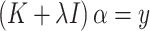(5)

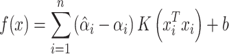
where K is a kernel matrix, whose elements represent kernel values between training samples; I is an identity matrix; and α is the vector of coefficients being estimated to predict new inputs. For a new input x, the predicted value can be calculated using the following formula:

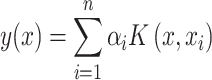(6)

where α_i is an element in the vector α obtained from the above solution, and is the ith individual in the training sample. The Python software package ‘Sklearn’ [20] was used to implement the prediction process of K_PRR, using a grid search method to find the best parameters of the polynomial kernel.

S_PVR

Support vector regression classifies samples by finding a hyperplane that best separates different categories in the sample space. The core idea is to minimize prediction error while maximizing the margin between the hyperplane and the data points. Some errors are tolerated in the process. Specifically, we assume that a deviation of between f(x) and y_i is acceptable, meaning that the loss is only calculated when the gap between f(x) and y_i exceeds . The SVR problem can be formalized as:

(7)

where c is a regularization constant and is the ε-insensitive loss function, the loss was calculated only if the absolute value of the difference between f(x_i) and y_i exceeds the threshold ε:

(8)

After adding slack variables and Lagrangian multipliers, the partial derivative of the loss function can be obtained:

(9)

After mapping the data:

(10)

(11)

where is the kernel function, and are positive weights given to each observation and estimated from the data and inner product kernel is an symmetric and positive definite matrix. The Python software package ‘Sklearn’ [20] was used to implement the prediction process of S_PVR.

BayesB

The statistical model can be written as:

(12)

where y is the vector of phenotypic values; μ is the overall mean; is the genotype of the j-th marker locus; is the effect of the j-th marker following and with probability π and (1-π), respectively; e is the vector of random residuals that are assumed to be normally distributed where I is an identity matrix and is the residual variance; p is the total number of markers. The R package ‘BGLR’ was used to implement BayesB.

GBLUP

The statistical model can be written as:

(13)

where is the vector of phenotypic values; b is a vector of fixed effects, X is a design matrix relating the fixed effects; is the vector of random additive genetic effects that are assumed to be normally distributed as where G is a marker-based genomic relationship matrix and is the additive genetic variance; Z is an incidence matrix of ; and e is the vector of random residuals that were assumed to be normally distributed as where I is an identity matrix and is the residual variance. In this context, the G matrix was constructed according to VanRaden [21] and the R package ‘sommer’ was used to implement GBLUP [22].

GDBLUP

This method included additive and dominance effects as random effects. The statistical model can be written as:

(14)

where is the vector of dominance effects that are assumed to be normally distributed as where D is the dominance genomic relationship matrix and is the dominant variance; is the incidence matrix of ; and other elements are the same as the GBLUP model. The R package ‘sommer’ was used to construct the D matrix and implement GDBLUP [22].

GEBLUP

This method included additive and epistatic effects as random effects. The statistical model can be written as:

(15)

where is the vector of the epistatic effects that are assumed to be normally distributed as where is the epistatic genomic relationship matrix and is the dominance genetic variance; is the incidence matrix of ; other elements are the same as the GBLUP model. It should be mentioned that is constructed using the equation where # denotes the Hadamard product operation and the R package ‘sommer’ was used to implement GEBLUP [22].

DeepGS

DeepGS was implemented using the graphics-processing-unit (GPU)-based deep learning framework mxnet (version 0.7.0; https://github.com/dmlc/mxnet); DeepGS is provided as an open-source R package available at https://github.com/cma2015/DeepGS. More details on this method were presented in Ma et al. [23].

Datasets

To evaluate performance of K_PRR in comparison to other methods, we analyzed six publicly available datasets. In brief, these datasets are as follows.

Wheat dataset

This dataset includes 599 wheat lines from a global wheat programme of the International Maize and Wheat Improvement Centre, which conducted trials across a wide range of wheat producing environments that were grouped into four basic target sets of environments [24]. They were genotyped using the 1447 Diversity Array Technology platform, which takes on two values to denote their presence (1) or absence (0). Markers with a minor allele frequency <0.05 were removed, and missing genotypes were imputed based on the marginal distribution of marker genotypes. There were 1279 markers retained after these quality controls. This dataset is accessible through the R package ‘BGLR’ [25], where W1, W2, W3, and W4 represent the four traits. All phenotypic values were standardized to a unit variance.

German Holstein cattle

The German Holstein cattle dataset comprised 5024 bulls genotyped with the Illumina Bovine SNP50 BeadChip. After quality control, 42 551 SNPs remained for further analysis [26]. Conventional estimated breeding values of milk yield (MY), milk fat percentage (MFP), and somatic cell score (SCS) were available for all bulls. Building on the well-established knowledge from previous studies [27, 28], these are complex traits representing three distinct genetics architectures. The MFP trait has high heritability, and the variation is dominated by one major gene (DGAT1, the diacylglycerol acyltransferase 1) in conjunction with a large number of other genes and genomic regulatory elements (GREs) with small effects. The MY trait has moderate heritability and is partly determined by DGAT1 and many genes and GREs with medium and small effects. The SCS trait is a low heritability trait and is influenced by a large number of genes and GREs with small effects [29]. The phenotypic values representing SCS were transformed to follow normal distributions. Additional details on this dataset are available in Zhang et al. [26].

Pig dataset

This comprised 3534 animals from a Pig Improvement Company (PIC) nucleus pig line encompassing a total of five traits. These animals had genotypes from Illumina PorcineSNP60 chips. SNPs with Hardy–Weinberg equilibrium test P-value <10⁻⁴, genotype call rate <95%, and minor allele frequency <0.05 were discarded. After quality control, 38 891 SNPs and 2314 animals with phenotypes remained. According to the reported heritabilities [30], we selected three representative traits of T2 (h² = 0.16), T3 (h² = 0.38), and T4 (h² = 0.58) to conduct analyses. The dominance variances of these traits had been reported to be 2%, 7%, and 1%, respectively [31]. The phenotypic values were pre-adjusted by fixed effects or were weighted progeny mean–corrected phenotypes.

Sheep dataset

This consisted of 752 Scottish Blackface sheep, bred over a 3-year period with both sire and dam recorded at birth for all animals, and a complete pedigree available back to the foundation of the flock in 1988. Additional information on the rearing and management procedures is provided by Riggio et al. [32]. The dataset includes three live weight traits: body weights at 16 weeks (BW16), at 20 weeks (BW20), and at 24 weeks (BW24). Phenotypic values were pre-adjusted for sex, year, age of dam, and group. After quality control, a total of 37 243 SNPs were retained for further analysis. The dominance variances accounted for 38%, 6%, and 30% of the total phenotypic variance for BW16, BW20, and BW24, respectively [33].

Simulation dataset

This dataset includes 600 individuals from a simulated backcross population with a single large chromosome covered by 121 evenly spaced markers [34]. Nine of the markers overlapped with QTLs affecting additive effects, while 13 out of the possible marker pairs exhibited interaction effects. Detailed information on the dataset and the true effects of the markers or marker pairs can be found in Xu [34]. The fixed effect accounted for the population mean, while the phenotypic variance was attributed to main, epistatic, and residual effects.

Rice dataset

This dataset comprises an F2 population, which were collected in the 1998 and 1999 rice growing seasons from replicated field trials on an experimental farm [11]. It includes four traits: yield (Yield), number of tillers per plant (Tiller), number of grains per panicle (Grain), and 1000 grain weight (KWG). After quality control, 278 of all cross combinations were characterised by a phenotype and 1619 bin genotypes. The phenotypic values were pre-adjusted by the fixed year effects. Xu et al. [35] reported that these traits were controlled by additive and epistasis variances rather than by dominance variance, and epistasis variances of Yield, Tiller, Grain, and KWG were 95%, 69%, 52%, and 23%, respectively.

These six datasets contained 18 traits. All of them were known to be controlled by additive, dominance, or epistasis genetic effects. The details of all datasets are presented in Table 1.

Table 1.

Summary of all datasets.

Genetic effects	Dataset	Trait	N a	Meanb	SDb	r 2/h2c
Additive	Wheat	W1	599	0	1
		W2	599	0	1
		W3	599	0	1
		W4	599	0	1
	Holstein cattle	MY	5024	370.79	641.60	0.95
		MFP	5024	−0.06	0.28	0.94
		SCS	5024	102.32	11.73	0.88
Additive + dominance	Pig	T2	2314	0.06	1.12	0.16
		T3	2314	0.66	0.99	0.38
		T4	2314	1.04	2.39	0.58
	Sheep	BW16	707	−6.10	46.72	0.39
		BW20	464	−6.10	46.72	0.35
		BW24	734	6.02	48.83	0.23
Additive + epistasis	Simulation	Simulation	600	5.33	10.33	0.62
	Rice	Yield	278	0	5.83	0.38
		Tiller	278	0	1.56	0.50
		Grain	278	0	16.94	0.67
		KWG	278	0	1.76	0.84

^aThe number of individuals with phenotypes.

^bMean and standard error (SD) of phenotypic values.

^cReliability (r²) for cattle traits or heritability (h²) for other traits.

Model evaluation

Five replicates of a 5-fold validation cross-validation procedure were used to determine the prediction accuracy. Each dataset was randomly divided into five folds. Four folds were used as a training set with the remaining fold used for validation. The prediction accuracy was calculated for each validation fold by Pearson correlation:

(16)

where y is the adjusted phenotypic value and GEBV is the genomic estimated breeding value (or predicted value). The prediction accuracies for one replicate are the average Pearson correlation coefficients from the five folds.

Computing time were used to evaluate the computing efficiency of each method. All calculations were performed on the same research server (Ubuntu 18.04.6, 72 CPUs @ 2.30GHz), using the same threads and memory.

Results

Comparson of prediction accuracies in traits with additive genetic effects

Figure 1 illustrates the prediction accuracies for the two datasets including seven traits that were not controlled by nonadditive effects. Five methods—K_PRR, S_PVR, GBLUP, BayesB, and DeepGS—were used to predict the GEBVs for seven traits, consisting of four from the wheat dataset and three from the dairy cattle dataset. In the wheat dataset, prediction accuracies across all traits ranged from 0.354 to 0.544. Specifically, the prediction accuracies for trait W1 ranged from 0.502 to 0.544, for W2 from 0.425 to 0.491, for W3 from 0.354 to 0.389, and for W4 from 0.440 to 0.483. The prediction accuracies for each trait varied by 0.042, 0.066, 0.035, and 0.043, respectively, indicating a relatively stable performance across traits. K_PRR consistently achieved the highest predictive accuracies across all traits. For the Holstein cattle dataset, the prediction accuracies for trait MY ranged from 0.721 to 0.791, for MFP from 0.758 to 0.870, and for SCS from 0.676 to 0.742. The results varied slightly across different methods for all three traits, with the exception of BayesB, which significantly outperformed other methods in predicting MFP. Overall, BayesB achieved the highest prediction accuracies for traits MY and MFP, while K_PRR and GBLUP showed similar and stable performances for traits MY and MKG. For SCS, the prediction accuracies were nearly identical across all methods except for DeepGS. The details of the 5-fold cross-validation Pearson correlation coefficients are provided in Table S1.

Figure 1.

The prediction accuracies for traits influenced primarily by additive genetic effects for the wheat (left) and cattle (right) datasets. For each plot, the horizontal line represents the median value, and the upper and lower ends of each box represent the maximum and minimum.

Comparison of prediction accuracies in traits with additive and dominance effects

Figure 2 shows the prediction accuracies for the pig and sheep datasets, focusing on traits influenced by additive and dominance effects. Six methods—K_PRR, S_PVR, BayesB, GBLUP, GDBLUP, and DeepGS—were used to predict the GEBVs of all six traits, consisting of three from the pig dataset and three from the sheep dataset. In the pig dataset, prediction accuracies for T2 ranged from 0.460 to 0.497, for T3 from 0.311 to 0.323, and for T4 from 0.416 to 0.450. The differences in prediction accuracies between GDBLUP and GBLUP, K_PRR and GBLUP, and K_PRR and GDBLUP were all within ±0.02, indicating that the differences in prediction accuracies among the methods for this dataset were minimal. For the sheep dataset, the prediction accuracies for BW16 ranged from 0.189 to 0.261, for BW20 from 0.297 to 0.360, and for BW24 from 0.133 to 0.212. Overall, K_PRR and S_PVR achieved the highest prediction accuracies, while GBLUP performed the worst. Compared with GBLUP, GDBLUP achieved higher prediction accuracies with these three traits increased by 8%, decreased by 1%, and increased by 59%, respectively, due to the incorporation of the dominance effect in the model. Additionally, when comparing K_PRR with GDBLUP, the prediction accuracies of K_PRR improved by 37%, 18%, and 59% across the three traits. Furthermore, comparing K_PRR with GDBLUP, it was found that the prediction accuracies of K_PRR were improved by 26%, 19%, and 23%, respectively. The details of the 5-fold cross-validation Pearson correlation coefficients are provided in Table S1.

Figure 2.

The prediction accuracies of datasets under the additive and dominance genetic background, including PIC pig and Scottish sheep datasets. For each box, the horizontal line represents the median value, and the upper and lower ends of each box represent the maximum and minimum.

Comparson of prediction accuracies in traits with additive and epistasis effects

Figure 3 shows the prediction accuracies for the simulated and rice datasets including five traits that are influenced by additive and epistatic effects. The methods of K_PRR, S_PVR, BayesB, GBLUP, GEBLUP, and DeepGS were employed to analyse all five traits, consisting of one from the simulated dataset and four from the rice dataset. The prediction accuracies for the simulated trait ranged from 0.501 to 0.768, with the methods ranked in the following order: K_PRR > GEBLUP > BayesB > GBLUP > S_PVR > DeepGS. In the rice dataset, prediction accuracies ranged from 0.363 to 0.417 for Yield, 0.373 to 0.509 for Tiller, 0.490 to 0.626 for Grain, and 0.759 to 0.748 for KGW. K_PRR outperformed other methods for the simulated traits, as well as Yield and Tiller. For Grain and KWG, BayesB yielded the highest prediction accuracy. Overall, S_PVR and DeepGS showed the lowest performance across the datasets.

Figure 3.

The prediction accuracies of datasets under the additive and epistasis genetic background, including simulated and rice datasets. For each box, the horizontal line represents the median value for the average correlation, and the upper and lower ends of each box represent replicates with the maximum and minimum average correlations.

Compared to GBLUP, GEBLUP showed that the improvement in prediction accuracies from including epistasis varied across different traits. Specifically, the prediction accuracies for the simulated trait, Yield and Grain, increased by 23%, 7%, and 2%, respectively. However, the prediction accuracies for Tiller decreased by 2%, and KWG remained unchanged. In comparison with GBLUP, the prediction accuracies of K_PRR increased by 24%, 12%, 2%, 3%, and 0% for these five traits, respectively. When compared with GEBLUP, K_PRR’s prediction accuracies were higher by 1%, 5%, 4%, 1%, and 0% for these traits, respectively. These results indicated that K_PRR can effectively account for epistatic effects and achieved improved prediction performance without relying on an explicit epistasis effect. The details of the 5-fold cross-validation Pearson correlation coefficients are provided in Table S1.

Comparison of computing time

The computing time for the wheat dataset ranged from 1 to 318 s, for the Holstein cattle dataset from 154 to 33 071 s, for the simulation dataset from 0 to 1081 s, and for the rice dataset from 0 to 1099 s. In the pig dataset, running times ranged from 149 to 227 856 s, while in the sheep dataset, they ranged from 8 to 31 985 s. Figure 4 illustrates the computing times for the different methods, with the values transformed to a log₁₀ scale. As expected, the computing time increased with the number of individuals or SNPs for all methods. Among all traits, K_PRR required the least computation time, while BayesB consistently took the most. For rice traits, K_PRR was ~2500 times faster than BayesB. In both the simulated and rice datasets, S_PVR required less computing time than GBLUP, whereas in the pig and sheep datasets, it took more. It is worth noting that computation time for deep learning method were not presented in this study, as DeepGS required more advanced hardware configuration (GPU). The details of the running time are provided in Table S2.

Figure 4.

Comparisons of computing time (in log₁₀-transformed seconds) for K_PRR, S_PVR, BayesB, GBLUP, GEBLUP, and GDBLUP for all datasets.

Discussion

The performance of genomic prediction methods varies according to the nature of the genetic architecture, the number of loci responsible, and the population structure [36]. We found that no single method consistently outperforms others across all traits, and each method has its own unique advantages. K_PRR outperformed the other methods in most of traits analyzed. BayesB showed the best performance for traits MY and MFP regulated by main gene DGAT1, which further validated that its strong capability in predicting traits controlled by large-effect genes or QTLs [37]. By incorporating nonadditive effects, the conventional best linear unbiased prediction (BLUP) model can achieve better predictive performance compared to models that considered only additive effects. When dominance and epistatic effects were integrated into the GBLUP model to create the GDBLUP and GEBLUP models, both models exhibited significantly higher prediction accuracies compared to GBLUP in datasets with the traits influenced by nonadditive effects. This phenomenon was also observed in cassava populations, where the predictive performance improved by 10% after fitting nonadditive effects into the model for seven traits [13]. In this study, the genomic prediction accuracies for four traits in the wheat dataset were 0.507, 0.487, 0.385, and 0.461, respectively, which were consistent with the values reported in the original paper (0.512, 0.483, 0.401, and 0.463) [24]. Similarly, the genomic prediction accuracies for three traits in the cattle dataset using GBLUP in our study were 0.772, 0.816, and 0.740, respectively, which were in agreement with those reported in original paper (0.774, 0.816, and 0.738) [26].

In this study, K_PRR ML strategy effectively captured both additive and nonadditive effects in some datasets, enhancing the accuracy of genomic prediction models. When analyzing the traits controlled solely by additive effects, K_PRR outperformed four other methods (S_PVR, BayesB, GBLUP, and DeepGS) for all four traits in the wheat dataset, whereas for the three traits in the cattle dataset, K_PRR achieved prediction accuracies similar to GBLUP. Although K_PRR showed some advantages in capturing nonadditive effects, it did not show better performance than traditional methods when the proportion of dominance variance were low, as observed for the three traits in the pig dataset (2%, 7%, and 1%). This limited contribution of dominance effects may explain why K_PRR did not significantly outperform other methods and why GDBLUP showed only minor improvements compared to GBLUP. In contrast, the sheep dataset exhibited higher dominance variances accounting for 38%, 6%, and 30% of the total phenotypic variation for the three traits. In this dataset, K_PRR consistently outperformed other methods, demonstrating that its advantage becomes more pronounced as the proportion of dominance effects increases. In the simulated dataset, 13 possible label pairs exhibited interactive effects, which contributed to a high proportion of epistatic variance. K_PRR performed the best, followed by GEBLUP, BayesB, GBLUP, and S_PVR. The relatively higher epistatic variance contributing to the four traits in the rice dataset may explain why K_PRR showed the greatest advantages. This suggested that the effectiveness of K_PRR may vary depending on different genetic backgrounds and traits analyzed. Meanwhile, the choice of kernel function needs to be based on prior experience or trial and error, which complicates model selection. However, kernel selection and parameter tuning can be facilitated by methods such as grid search or Bayesian optimization [38]. Furthermore, the generalization ability of K_PRR is worthy of further study. While K_PRR performed well on the datasets in this study, its ability to adapt to and predict new data still required validation.

Notable differences in computational efficiency were observed among the methods. BayesB required the longest computation time for all traits. Among Bayesian alphabet methods, we chose BayesB because it was the first method used in genomic prediction [1]. However, Bayesian alphabets rely on Markov chain Monte Carlo sampling algorithms, which are time consuming, especially for large models with extensive sample sizes. In contrast, K_PRR required the least computation time and is sometimes thousands of times faster than other methods. This speed advantage may be related to the characteristics of the K_PRR algorithm. First, kernel ridge regression can use closed solutions to estimate model parameters, which suggests that the model can directly obtain the optimal solution without iterative optimization [39]. Second, the regularization term in kernel ridge regression makes the model more inclined to use low-dimensional feature subspaces to reduce complex computational complexity. We also noted that the running time of S_PVR was always longer than K_PRR, despite both being kernel-based methods. This difference arises from their distinct optimization approaches. Based on the principle of support vector machine, S_PVR minimizes the prediction error by constructing an optimal hyperplane. The process of finding that hyperplane involves solving a convex quadratic programming problem, that is, a series of inequality constraints must be satisfied while optimizing the loss function [39]. Convex quadratic programming problems are often complex to solve, so the running time of S_PVR can be extensive with large datasets. In this study, we did not record the running time of the DeepGS method. That is because the DeepGS method requires high computer specifications, including a GPU. If using a single-machine version, it would take nearly a month, as the computation times are not on the same level, making it impossible to compare their durations directly. Nevertheless, in this study, DeepGS did not show any advantages among all methods. The reason might be that we used the default parameters in the DeepGS R package. Another possible reason is the limited sample sizes used in our study.

Future studies could explore the mechanisms underlying the nonadditive genetic effects and their impact on prediction method performances, which can pave the way for the development of customized algorithms optimized for specific traits. Additionally, exploring additional kernel functions, and fine-tuning model parameters could further improve the accuracy of genomic prediction. Beyond genomic data, multi-omics data, such as transcriptomics and metabolomics, can be added to the genomic prediction models, which holds great potential. Currently, some related studies have shown that ML has certain advantages for multi-omics integration [40, 41]. With the rapid development of high-throughput sequencing and various other molecular techniques, integrating these omics data to improve prediction accuracy has become an important scientific problem.

Conclusion

In this study, we proposed an ML strategy, K_PRR, based on kernel ridge regression with a polynomial kernel function. The performance of K_PRR was compared against six other genomic prediction methods on datasets with different genetic architectures. The results show that (i) for traits dominated by additive effects, the K_PRR exhibited similar predictive accuracy to the traditional genomic selection methods GBLUP and BayesB. However, when traits are controlled by large effect genes, the BayesB method outperformed the others in terms of prediction accuracy. (ii) For traits influenced by additive and non-additive effects, the inclusion of dominance or epistasis effects improved prediction accuracy for the GBLUP model. However, K_PRR maintained equal or higher prediction accuracy, which illustrates the advantages of ML in transforming high-dimensional feature spaces and capturing nonadditive effects. (iii) K_PRR required the shortest overall computing time, while the BayesB method was the most computationally intensive. In summary, this study demonstrated that ML strategies can improve genomic prediction across diverse plant and livestock datasets in complex genetic backgrounds. These findings provide valuable insights for optimizing breeding strategies across species and traits.

Key Points

• We introduced a novel machine learning strategy, K_PRR, which integrated a polynomial kernel with ridge regression to improve genomic prediction accuracy.

• K_PRR demonstrated certain improvements in capturing nonadditive genetic effects, including epistasis and dominance, over traditional genomic prediction methods.

• The effectiveness of K_PRR is validated empirically across multiple datasets, showing its robustness in both plant and animal genomic predictions.

• K_PRR not only improved prediction accuracy but also offers advantages in computational efficiency, consistently outperforming the other methods in terms of computational speed.

 

Conf lict of interest: The authors declare no conflict of interest.

Funding

This work was funded by National Natural Science Foundations of China (No. 32172702), State Key Laboratory of Animal Biotech Breeding (XQSWYZQZ-KFYX-4), the National Key Research and Development Program of China (2021YFD1301102, 2024YFF1000100) and Agricultural Science and Technology Innovation Program (ASTIP-IAS02). M.L. was supported by the China Scholarship Council for a 1-year study period at University College Dublin.

Data availability

Wheat dataset: https://rdrr.io/cran/BGLR/man/wheat.html, German Holstein cattle: https://academic.oup.com/g3journal/article/5/4/615/6025251?login=true#supplementary-data, Simulation dataset: http://www.tibs.org/biometrics, Rice dataset: https://www.pnas.org/doi/full/10.1073/pnas.1413750111#supplementary-materials, Pig dataset: https://academic.oup.com/g3journal/article/2/4/429/6026060#supplementary-data, Sheep dataset: https://datadryad.org/stash/dataset/doi:10.5061/dryad.8f191.

Author contributions

Conceptualization: F.Z., L.W.; Methodology: F.Z., M.L.; Data Analysis: M.L., L.C.; Writing—Original Draft Preparation: M.L., L.C.; Writing—Review & Editing: F.Z., T.H., D.E.M., D.G.; Supervision: F.Z., D.E.M.

References

- 1. Meuwissen TH, Hayes BJ, Goddard ME. Prediction of total genetic value using genome-wide dense marker maps. Genetics 2001;157:1819–29. 10.1093/genetics/157.4.1819. [DOI] [PMC free article] [PubMed] [Google Scholar]
- 2. Weller JI, Ezra E, Ron M. Invited review: A perspective on the future of genomic selection in dairy cattle. J Dairy Sci 2017;100:8633–44. 10.3168/jds.2017-12879. [DOI] [PubMed] [Google Scholar]
- 3. Alemu A, Astrand J, Montesinos-Lopez OA. et al. Genomic selection in plant breeding: Key factors shaping two decades of progress. Mol Plant 2024;17:552–78. 10.1016/j.molp.2024.03.007. [DOI] [PubMed] [Google Scholar]
- 4. Meuwissen TH, Hayes BJ, Goddard M. Genomic selection: A paradigm shift in animal breeding. Anim Front 2016;6:6–14. 10.2527/af.2016-0002. [DOI] [Google Scholar]
- 5. Garcia-Ruiz A, Cole JB, VanRaden PM. et al. Changes in genetic selection differentials and generation intervals in US Holstein dairy cattle as a result of genomic selection. Proc Natl Acad Sci USA 2016;113:E3995–4004. 10.1073/pnas.1519061113. [DOI] [PMC free article] [PubMed] [Google Scholar]
- 6. Falconer DS, Mackay TF. Introduction to Quantitative Genetics (4th ed.). Harlow, Essex, UK: Longmans Green, 1996. [Google Scholar]
- 7. Xu S. Quantitative Genetics. Switzerland: Springer Cham, 2022, 10.1007/978-3-030-83940-6. [DOI] [Google Scholar]
- 8. Mackay TFC, Anholt RRH. Pleiotropy, epistasis and the genetic architecture of quantitative traits. Nat Rev Genet 2024;25:639–57. 10.1038/s41576-024-00711-3. [DOI] [PMC free article] [PubMed] [Google Scholar]
- 9. Bernardo R, Yu J. Prospects for genomewide selection for quantitative traits in maize. Crop Sci 2007;47:1082–90. 10.2135/cropsci2006.11.0690. [DOI] [Google Scholar]
- 10. Calus MP, Meuwissen TH, Roos AP. et al. Accuracy of genomic selection using different methods to define haplotypes. Genetics 2008;178:553–61. 10.1534/genetics.107.080838. [DOI] [PMC free article] [PubMed] [Google Scholar]
- 11. Yu S, Li J, Xu C. et al. Importance of epistasis as the genetic basis of heterosis in an elite rice hybrid. Proc Natl Acad Sci USA 1997;94:9226–31. [DOI] [PMC free article] [PubMed] [Google Scholar]
- 12. Costa E, Silva J, Borralho NM. et al. Additive and non-additive genetic parameters from clonally replicated and seedling progenies of Eucalyptus globulus. Theor Appl Genet 2004;108:1113–9. 10.1007/s00122-003-1524-5. [DOI] [PubMed] [Google Scholar]
- 13. Wolfe MD, Kulakow P, Rabbi IY. et al. Marker-based estimates reveal significant nonadditive effects in clonally propagated cassava (Manihot esculenta): Implications for the prediction of total genetic value and the selection of varieties. G3-Genes Genom Genet 2016;6:3497–506. 10.1534/g3.116.033332. [DOI] [PMC free article] [PubMed] [Google Scholar]
- 14. Akdemir D, Jannink J-L, Isidro-Sánchez J. Locally epistatic models for genome-wide prediction and association by importance sampling. Genet Sel Evol 2017;49:1–14. 10.1186/s12711-017-0348-8. [DOI] [PMC free article] [PubMed] [Google Scholar]
- 15. Akdemir D, Jannink J-L. Locally epistatic genomic relationship matrices for genomic association and prediction. Genetics 2015;199:857–71. 10.1534/genetics.114.173658. [DOI] [PMC free article] [PubMed] [Google Scholar]
- 16. Lopez OAM, Lopez AM, Crossa J. Multivariate Statistical Machine Learning Methods for Genomic Prediction. Switzerland: Springer Cham, 2022, 10.1007/978-3-030-89010-0. [DOI] [PubMed] [Google Scholar]
- 17. Suzuki J. Kernel Methods for Machine Learning with Math and Python. Singapore: Springer nature, 2022, 10.1007/978-981-19-0401-1. [DOI] [Google Scholar]
- 18. An B, Liang M, Chang T. et al. KCRR: A nonlinear machine learning with a modified genomic similarity matrix improved the genomic prediction efficiency. Brief Bioinform 2021;22:bbab132. 10.1093/bib/bbab132. [DOI] [PubMed] [Google Scholar]
- 19. Zhao W, Lai X, Liu D. et al. Applications of support vector machine in genomic prediction in pig and maize populations. Front Genet 2020;11:598318. 10.3389/fgene.2020.598318. [DOI] [PMC free article] [PubMed] [Google Scholar]
- 20. Pedregosa F, Varoquaux G, Gramfort A. et al. Scikit-learn: Machine learning in python. J Mach Learn Res 2011;12:2825–30. 10.1093/bib/bbab132. [DOI] [Google Scholar]
- 21. VanRaden PM. Efficient methods to compute genomic predictions. J Dairy Sci 2008;91:4414–23. 10.3168/jds.2007-0980. [DOI] [PubMed] [Google Scholar]
- 22. Covarrubias-Pazaran G. Genome-assisted prediction of quantitative traits using the R package sommer. PLoS One 2016; 11:e0156744. 10.1371/journal.pone.0156744. [DOI] [PMC free article] [PubMed] [Google Scholar]
- 23. Ma W, Qiu Z, Song J. et al. A deep convolutional neural network approach for predicting phenotypes from genotypes. Planta 2018;248:1307–18. 10.1007/s00425-018-2976-9. [DOI] [PubMed] [Google Scholar]
- 24. Crossa J, Campos Gde L, Perez P. et al. Prediction of genetic values of quantitative traits in plant breeding using pedigree and molecular markers. Genetics 2010;186:713–24. 10.1534/genetics.110.118521. [DOI] [PMC free article] [PubMed] [Google Scholar]
- 25. P dlCGP. BLR: Bayesian linear regression. R-package version 1.2 . https://cran.r-project.org/web/packages/BLR/index.html.
- 26. Zhang Z, Erbe M, He J. et al. Accuracy of whole-genome prediction using a genetic architecture-enhanced variance-covariance matrix. G3-Genes Genom Genet 2015;5:615–27. 10.1534/g3.114.016261. [DOI] [PMC free article] [PubMed] [Google Scholar]
- 27. Hu ZL, Park CA, Wu XL. et al. Animal QTLdb: An improved database tool for livestock animal QTL/association data dissemination in the post-genome era. Nucleic Acids Res 2013;41:D871–9. 10.1093/nar/gks1150. [DOI] [PMC free article] [PubMed] [Google Scholar]
- 28. Zhang Z, Ober U, Erbe M. et al. Improving the accuracy of whole genome prediction for complex traits using the results of genome wide association studies. PLoS One 2014;9:e93017. 10.1371/journal.pone.0116056. [DOI] [PMC free article] [PubMed] [Google Scholar]
- 29. Yin L, Zhang H, Zhou X. et al. KAML: Improving genomic prediction accuracy of complex traits using machine learning determined parameters. Genome Biol 2020;21:1–22. 10.1186/s13059-020-02052-w. [DOI] [PMC free article] [PubMed] [Google Scholar]
- 30. Cleveland MA, Hickey JM, Forni S. A common dataset for genomic analysis of livestock populations. G3-Genes Genom Genet 2012;2:429–35. 10.1534/g3.111.001453. [DOI] [PMC free article] [PubMed] [Google Scholar]
- 31. Da Y, Wang C, Wang S. et al. Mixed model methods for genomic prediction and variance component estimation of additive and dominance effects using SNP markers. PLoS One 2014;9:e87666. 10.1371/journal.pone.0087666. [DOI] [PMC free article] [PubMed] [Google Scholar]
- 32. Riggio V, Matika O, Pong-Wong R. et al. Genome-wide association and regional heritability mapping to identify loci underlying variation in nematode resistance and body weight in Scottish blackface lambs. Heredity 2013;110:420–9. 10.1038/hdy.2012.90. [DOI] [PMC free article] [PubMed] [Google Scholar]
- 33. Alipanah M, Roudbari Z, Momen M. et al. Impact of inclusion non-additive effects on genome-wide association and variance’s components in Scottish black sheep. Anim Biotechnol 2023;34:3765–73. 10.1080/10495398.2023.2224845. [DOI] [PubMed] [Google Scholar]
- 34. Xu S. An empirical bayes method for estimating epistatic effects of quantitative trait loci. Biometrics 2007;63:513–21. 10.1111/j.1541-0420.2006.00711.x. [DOI] [PubMed] [Google Scholar]
- 35. Xu S, Zhu D, Zhang Q. Predicting hybrid performance in rice using genomic best linear unbiased prediction. Proc Natl Acad Sci USA 2014;111:12456–61. 10.1073/pnas.1413750111. [DOI] [PMC free article] [PubMed] [Google Scholar]
- 36. Guo X, Christensen OF, Ostersen T. et al. Improving genetic evaluation of litter size and piglet mortality for both genotyped and nongenotyped individuals using a single-step method. J Anim Sci 2015;93:503–12. 10.2527/jas.2014-8331. [DOI] [PubMed] [Google Scholar]
- 37. Meher PK, Rustgi S, Kumar A. Performance of Bayesian and BLUP alphabets for genomic prediction: Analysis, comparison and results. Heredity 2022;128:519–30. 10.1038/s41437-022-00539-9. [DOI] [PMC free article] [PubMed] [Google Scholar]
- 38. Yang L, Shami A. On hyperparameter optimization of machine learning algorithms: Theory and practice. Neurocomputing 2020;415:295–316. 10.1016/j.neucom.2020.07.061. [DOI] [Google Scholar]
- 39. Schölkopf B, Smola A. Learning with kernels: Support vector machines, regularization, optimization, and beyond. Edited by Dietterich T. Cambridge, MA: MIT press, 2001, 10.7551/mitpress/4175.001.0001. [DOI] [Google Scholar]
- 40. Ye S, Li J, Zhang Z. Multi-omics-data-assisted genomic feature markers preselection improves the accuracy of genomic prediction. J Anim Sci Biotechnol 2020;11:109. 10.1186/s40104-020-00515-5. [DOI] [PMC free article] [PubMed] [Google Scholar]
- 41. Lin E, Lane H-Y. Machine learning and systems genomics approaches for multi-omics data. Biomark Res 2017;5:2. 10.1186/s40364-017-0082-y. [DOI] [PMC free article] [PubMed] [Google Scholar]
Associated Data
This section collects any data citations, data availability statements, or supplementary materials included in this article.
Supplementary Materials
Data Availability Statement