Type 2 diabetes prediction method based on dual-teacher knowledge distillation and feature enhancement

Abstract

Diabetes prediction is an important topic in the field of medical health. Accurate prediction can help early intervention and reduce patients’ health risks and medical costs. This paper proposes a data preprocessing method, including removing outliers, filling missing values, and using sparse autoencoder (SAE) feature enhancement. This study proposes a new method for type 2 diabetes classification using a dual Convolutional Neural Network (CNN) teacher-student distillation model (DCTSD-Model), aiming to improve the accuracy and reliability of diabetes prediction. The variables of the original data are expanded by SAE to enhance the expressive power of the features. The proposed CNN and DCTSD-Model models are evaluated on the feature enhancement dataset using 10-fold cross validation. The experimental results show that after data preprocessing, DCTSD-Model adopts the dual teacher model knowledge distillation method to help the student model learn rich category information by generating soft labels, and uses weighted random samplers to learn samples of different categories, which solves the category imbalance problem and achieves excellent classification performance. The accuracy of DCTSD-Model on the classification task reached 98.57%, which is significantly higher than other models, showing higher classification ability and reliability. This method provides an effective solution for diabetes prediction and lays a solid foundation for further research and application.

Introduction

Diabetes is a chronic disease with persistent hyperglycemia¹. Diabetes is mainly divided into type 1 diabetes mellitus (T1DM)², type 2 diabetes mellitus (T2DM)³ and gestational diabetes mellitus (GDM)⁴. T2DM accounts for about 90%-95% of all diabetes cases⁵. It is a heterogeneous and progressive disease caused by the combined effects of genetic and environmental factors⁶. Studies have shown that “thrifty genes” that gave people a survival advantage in resource-scarce environments in the past may have adverse effects on health in modern high-sugar, high-fat environments⁷. The hyperglycemia in T2DM usually results from an absolute or relative deficiency of insulin, mainly due to the failure to effectively compensate for insulin resistance⁸. Although we have a deeper understanding of the pathogenic mechanism and risk factors of T2DM and some effective preventive measures have been proposed, the incidence and prevalence of T2DM continue to rise worldwide⁹. According to data from the Global Burden of Disease Study, the age-standardized prevalence of T2DM in the world in 2019 was 5282.9 per 100,000 population, and the mortality rate was 18.5 per 100,000 population, an increase of 49% and 10.8% respectively from 1990. At the same time, the disability-adjusted life years (DALYs) associated with T2DM also increased by 27.6% during the same period¹⁰. This shows that although we have made some progress in the prevention and control of diabetes, the challenges facing global public health remain enormous in the face of rising prevalence rates.

T2DM usually lurks in the body for many years and often has no obvious symptoms in the early stages, but as the disease progresses, patients may develop serious complications such as cardiovascular disease, renal failure, vision loss and neuropathy. Therefore, early recognition and intervention are crucial. Early screening can buy valuable time for timely diagnosis. Through lifestyle intervention, drug treatment and other means, it can effectively delay or even reverse the progression of the disease, thereby significantly improving the patient’s quality of life and reducing the occurrence of complications. At the same time, different patients with T2DM have differences in disease progression and response to treatment. Accurate classification prediction is of great significance for developing individualized treatment plans. Classification prediction helps doctors adjust treatment strategies according to the specific conditions of patients and choose the most appropriate treatment method, thereby optimizing treatment effects, reducing side effects, and avoiding unnecessary treatment, which is crucial to improving patients’ clinical outcomes.

In recent years, with the advancement of data science and machine learning(ML) technologies, the use of these technologies to improve the diagnosis and prediction of T2DM has shown significant effectiveness. In 2020, Hasan et al.¹¹ proposed a powerful diabetes prediction framework that combines outlier rejection, feature selection, and multiple ML classifiers. By combining different ML models and optimizing the prediction based on Area Under the Curve(AUC) weighting, the combined classifier achieved an AUC of 95% on the Pima Indians Diabetes(PID) database, significantly outperforming existing methods. Khanam et al.¹² used ML and Neural Networks(NN) methods to predict diabetes in 2021. Using the PID dataset, the combination of Logistic Regression(LR) and Support Vector Machine(SVM) models achieved the best results, and the accuracy of the NN model with two hidden layers reached 88.6%. In 2022, Olisah et al.¹³ used Spearman correlation and polynomial regression for selecting features and handling missing values. Their Two-Gradient Descent Neural Network(2GDNN) model attained a 97.25% accuracy on the PID dataset. In addition, ensemble learning and other ML techniques have also made significant progress in diabetes prediction. In 2022, Ahmed et al.¹⁴ proposed the FMDP model that integrates machine learning methods for diabetes prediction. By combining SVM and ANN to analyze the dataset, the prediction accuracy of the FMDP model reached 94.87%. In 2023, Zhou et al.¹⁵ proposed a diabetes prediction model based on Boruta feature selection and ensemble learning(DPMBFSEL), with an accuracy of 98% on the PID dataset, which is better than other models. Doğru et al.¹⁶ proposed a super learning model in 2023, which improved the accuracy of early diagnosis of diabetes by integrating multiple algorithms, reaching 92% on the PID dataset, which is better than traditional methods. Alghamdi et al.¹⁷ used the XGBoost classifier in 2023 and achieved excellent performance in processing high-dimensional feature data, with an accuracy rate of 89% in predicting diabetes.

While traditional ML approaches have shown effectiveness, they face several challenges, including difficulty in handling class imbalance, heavy reliance on feature engineering, and extensive data preprocessing. These limitations reduce adaptability to diverse clinical data and hinder generalization across different datasets. Thus, there is a need for more advanced techniques that can address these issues, improve model robustness, and enhance adaptability in clinical settings.

Deep learning technology also shows great potential in diabetes prediction. In 2021, García-Ordás et al.¹⁸ proposed a deep learning technology based on variational autoencoder (VAE), sparse autoencoder (SAE) and CNN for diabetes prediction, achieving an accuracy of 92.31%. Bukhari et al.¹⁹ developed an improved artificial neural network (ANN) model using the back-propagation scaled conjugate gradient algorithm to predict diabetes on the PID dataset, which achieved an accuracy of 93%, outperforming other ANN models. In 2023, Aslan et al. ? proposed a diabetes prediction method that converts numerical data into images, using ResNet and SVM, with an accuracy of 92.19% on the PID dataset. In 2024, Zhao et al.²⁰ proposed a robust T2DM prediction framework in 2024. Using the NHANES and PID datasets, they optimized data preprocessing through the Attention-Oriented Convolutional Neural Network(SECNN) model and channel attention mechanism, significantly improving the prediction performance, with accuracy rates reaching 89.47% and 94.12%, respectively.

DL models outperform traditional ML techniques in handling complex data and learning representations automatically. However, they struggle with data class imbalance, which can lead to poor performance on minority classes. DL models also face challenges in generalizing across different clinical environments, requiring further optimization to improve their robustness and adaptability in diverse settings.

The studies above highlight significant progress in machine learning and deep learning for diabetes prediction, particularly in improving accuracy and optimizing data processing. However, challenges remain, particularly in addressing class imbalanceandmodel stability. Many models still struggle with poor performance on minority classes, impacting overall accuracy, and show performance variations across different datasets. Future research should focus on addressing these issues to improve model robustness, stability, and applicability in real-world clinical settings.

Based on this analysis, the contributions of this study are as follows:

• This study significantly improved the accuracy and reliability of data analysis by preprocessing the data, including filling missing values and using the IQR method to identify and process outliers. By replacing outliers with medians, the data distribution is more concentrated, reducing the impact of extreme values and ensuring the stability of subsequent analysis. After preprocessing, the normal distribution of the data is improved, and the correlation between the attributes becomes more significant, providing a more reliable data basis for subsequent statistical analysis and model building.

• This study expands the PID dataset from 8 independent variables to 200 variables by designing a SAE. The feature-enhanced dataset significantly improves the various indicators of the classification model in the 10-fold cross-validation evaluation.

• This study proposes a new diabetes classification model DCTSD-Model, which optimizes the category prediction ability by defining two teacher models and using a weighted random sampler. The soft labels generated by the teacher model are used for distillation training of the student model, significantly improving its generalization ability and classification performance. In the experiment, the accuracy of DCTSD-Model reached 98.58%, significantly better than other models.

Methodology

Research process

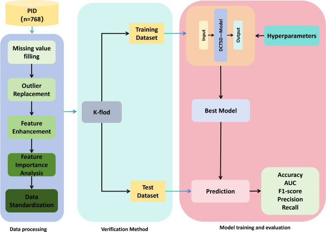
As shown in the Fig.  1, this study proposes a stable diabetes prediction workflow, which consists of three main components: data preprocessing, model validation, and evaluation. In the data preprocessing stage, we perform tasks such as missing value imputation, outlier handling, data augmentation, feature importance analysis, and data normalization to ensure the quality of the dataset and the effectiveness of model training. Next, for model validation, we employ five-fold cross-validation to ensure the model’s generalizability and stability. Finally, the model’s performance is comprehensively evaluated using five metrics: Accuracy, Recall, F1-score, Precision, and AUC. These metrics provide a well-rounded assessment of the model’s performance across different aspects, ensuring the accuracy and reliability of diabetes prediction.

Fig. 1.

Type 2 diabetes prediction flow chart.

Data

This study uses the publicly available Pima Indians Diabetes (PID) dataset. This dataset is widely used in diabetes prediction research. The dataset contains 8 independent variables and 1 dependent variable, covering a wide range, from clinical measurements to demographic information. These variables not only provide rich information for diabetes prediction, but also reflect various risk factors associated with diabetes. The target variable in the dataset is used to indicate whether each patient has diabetes, which serves as the basis for model training and evaluation.

Data preprocessing

Missing value filling

Missing values are a common problem in datasets²¹, which, if not handled properly, can lead to poor model performance or bias. Some samples in the PID dataset have missing values, especially features such as BMI, blood pressure, skinfold thickness, and insulin levels. To this end, we use the mean filling method to handle missing values. This helps reduce the interference of missing values on data distribution and maintain the uniformity of the dataset. For each feature, we first calculate the mean of the existing data and then use the mean to fill the corresponding missing values. The calculation formula is as follows

1

where is the non-missing value of the variable, and n represents the number of non-missing values of the variable.

Outlier identification and replacement

Outliers²² are data points that deviate significantly from the dataset. The reasons may be measurement errors, data entry errors, etc. Outliers can affect the training and prediction performance of the model, so it is very important to identify and replace outliers during the data preprocessing stage. In this study, we used the interquartile range (IQR) method to identify and handle these outliers. IQR is a statistic used to measure the degree of dispersion of data²³. IQR calculates the 25th percentile (Q1) and 75th percentile (Q3) of a dataset. The calculation formula for IQR is

2

Based on IQR, we can define the criteria for judging outliers. Generally, values outside the following range are considered outliers:

3

4

Data points outside the lower or upper bounds are considered outliers. For detected outliers, we replace them with the median of the feature. The median is the middle value of the data and is not affected by extreme values. It can effectively reduce the impact of outliers on the model. The processing steps are as follows:

• Calculate Q1 and Q3 for each feature.

• Calculate the IQR and determine the upper and lower bounds for outliers.

• Outliers outside the upper and lower bounds are replaced with the median of the feature.

Data standardization

Data normalization is an important step in ML²⁴, which aims to scale the feature data of the dataset to a certain range in order to improve the performance of the model. The standardization we used in this study is to subtract the mean of each feature value and divide it by its standard deviation, so that the processed data has a distribution with a mean of 0 and a standard deviation of 1. The standardization formula is as follows:

5

Among them, X is the original data, is the mean of the feature, and is the standard deviation of the feature.

Feature enhancement

Feature enhancement is an important method to improve the performance of ML models. By increasing the data dimension of the original features, the model can better capture the potential patterns and characteristics of the data. In this study, we perform feature augmentation on the PID dataset using sparse autoencoders (SAE) to generate new and more expressive features. SAE is a neural network model that uses unsupervised learning. Sparse autoencoder is an unsupervised learning neural network model²⁵ that learns the latent structure of data by encoding the input data into a low-dimensional representation and then decoding it back to the original data.Our sparse autoencoder consists of two parts: encoder and decoder. The specific structure is shown in Table 1. We also added sparsity constraints to the encoder part, so that the encoded representation can achieve feature selection and representation, reduce the risk of overfitting, and enhance data interpretability. This sparsity constraint is usually implemented by adding the Kullback-Leibler divergence (KL) as a regularization term, where the KL divergence can be expressed as

Table 1.

SAE structure description.

Part	Layer	Type	Input dimensions	Output dimensions	Activation function
Encoder	First	Linear layer	Number of features (input dimensions)	500	ReLU
Encoder	Second	Linear layer	500	Encoding dimension (100)	ReLU
Decoder	First	Linear layer	Encoding dimension (100)	500	ReLU
Decoder	Second	Linear layer	500	Number of features (input dimensions)	Sigmoid

6

where still represents the desired sparsity. represents the actual average activation value of the jth neuron. Mean square error (MSE) is used as the loss function, and it is combined with the sparsity regularization term for training, which can be expressed as

7

n is the number of training samples. is the weight of the sparsity regularization term, which controls the importance of the sparsity constraint. After training, new low-dimensional features are extracted and combined with the original features to form an enhanced feature set. This method improves the prediction performance and generalization ability of the model.

Feature importance analysis

In this study, we used one-way analysis of variance (ANOVA) to evaluate significant differences in extended features among different categories. Analysis of variance determines whether the mean difference of features between different categories is significant by calculating the p value. When the p value is less than 0.05, it means that the features are significantly different between different categories and may have a high contribution to the classification task. However, due to the large number of features, performing multiple comparisons may increase the risk of false positives. To control this problem, we used the Bonferroni correction method to adjust the p-value of each feature to ensure that the significance level of multiple comparisons remained within a reasonable range. Bonferroni correction reduces the occurrence of false positive results by dividing the significance level by the number of comparisons. It can be expressed as

8

where is the adjusted significance level (that is, the significance level of each individual test). is the original significance level. m is the number of comparisons made (i.e. the number of features). This correction method ensures that only those truly significant features are selected in multiple comparisons, further improving the reliability and interpretability of the model.

Model

Convolutional neural networks

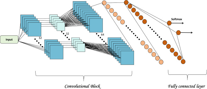
In this study, a convolutional neural network (CNN) was designed forT2DM classification. As shown in Fig.  2 , the network structure consists of two parts. The first part consists of two convolutional layers, each of which is followed by a ReLU activation function and a maximum pooling layer. The first convolutional layer has 32 output channels, while the second convolutional layer has 64 output channels. Both layers use 3x1 kernels and 1 edge padding to keep the data dimension unchanged. Through ReLU activation and max pooling layers, the network gradually extracts and compresses the features of the input data. The output of the convolutional layer is flattened and converted into a one-dimensional vector before being sent to the next stage. The first fully connected layer in this part is used for further feature learning, and the last fully connected layer outputs two nodes for classification. The output is converted to probability through the Softmax function to provide clear classification decisions. This network structure accurately learns key features through hierarchical processing and is suitable for scenarios that require fast and accurate classification.

Fig. 2.

CNN architecture.

Dual-CNN teacher–student distillation model (DCTSD-Model)

Knowledge distillation is a model compression technique that extracts knowledge from the teacher model and transfers it to the student model to improve the performance of the small model²⁶. It aims to utilize the high accuracy of the teacher model to guide the student model to learn more efficiently²⁷. The core idea of knowledge distillation is to use the soft labels generated by the teacher model as training data to assist the student model in learning. Soft labels not only contain the probability distribution information of the categories, but also reflect the similarity and uncertainty between categories. Compared with hard labels, soft labels provide richer training signals.

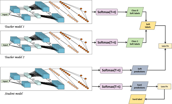
In response to the impact of the current data category imbalance problem on model performance and stability, this study proposed a new Dual-CNN Teacher-Student Distillation Model (DCTSD-Model). First, two CNNs are used as teacher models and trained for category 1 (diabetic patients) and category 0 (non-diabetic patients) respectively. This method has several advantages. First, training two teacher models separately can effectively reduce the impact of class imbalance on model training. Class 1 and class 0 are sampled independently by a weighted random sampler, so that each model focuses on its specific class of data, ensuring that the model can fully learn the characteristics of each class. Second, this approach improves model performance because each teacher model is able to better capture the data characteristics of that category, thereby generating more accurate soft labels to guide the learning of the student model. In addition, the two teacher models are trained for different categories separately, which helps to extract the features of their respective categories more finely, ensuring that each model can better understand the patterns and variability of its specific category when processing complex data. This training method also enhances the stability of the model. Since each model only needs to process a part of the data, it can reduce fluctuations during the training process and improve the stability and robustness of the model. Finally, training on a single category of data can simplify the optimization process and make it more focused and efficient. The specific training process includes initializing the optimizer. For each teacher model, the Adam optimizer is used for optimization, and the learning rate is set to 0.01. During the training process, the data of category 1 and category 0 were sampled, the loss was calculated, and the gradient was back-propagated to update the model parameters. The training process of the teacher model was carried out for a total of 1000 cycles to ensure that the model could fully learn the data characteristics of each category.

During distillation training, the student model uses the soft labels obtained from the teacher model as guidance. First, the teacher model is switched to evaluation mode and used to generate soft labels for the training data.Specifically, teacher model 1 generates soft labels for category 1 (diabetics) and teacher model 0 generates soft labels for category 0 (non-diabetics). These soft labels are obtained by forward propagating the training data through the teacher model. To train the student model, a new dataset is created, which includes the original input data and the corresponding soft labels. During the training process, the category 1 soft labels generated by teacher model 1 and the category 0 soft labels generated by teacher model 0 are taken separately and combined to construct a complete soft label set containing all the training data.

This method combines the soft labels generated by the two teacher models. The soft labels are calculated by the softmax function through the output logits of the teacher model. It can be expressed as

9

where is the soft label probability of category i; is the output logits of the teacher model on category i; T is the temperature parameter.The student model can learn the rich features of the two types of data and enhance the generalization ability of the model. Teacher Model 1 and Teacher Model 0 focus on the data of their respective categories, which enables the student model to better learn the specific information of each category. This method helps balance the class imbalance problem, allowing the student model to learn the characteristics of the two types of data more evenly and improve the overall model performance. By creating a complete training dataset, the training efficiency is also improved. In each training cycle, the input of the student model is the original training data, and the target is the soft label generated by the teacher model. By creating a complete training dataset, the training efficiency is also improved. In each training cycle, the input of the student model is the original training data, and the target is the soft label generated by the teacher model. By minimizing the KL divergence between the student model output and the soft label, the student model can effectively learn the rich feature information contained in the teacher model. During the distillation training of the student model, the loss function consists of two parts: KL divergence loss and cross entropy loss. The final total loss function L combines KL divergence and cross entropy loss.

10

where is the cross entropy loss, which measures the difference between the student model prediction and the true label y;e structure of the model is shown in Fig.  3.

Fig. 3.

DCTSD-model architecture.

Cross-validation

K-fold cross validation²⁸ is a widely used model validation method for evaluating the performance and generalization ability of machine learning models. This method divides the dataset into K non-overlapping subsets (called “folds”) and then performs K training and testing cycles. In each iteration, K-1 subsets are used for model training, and the remaining subset is used for testing. In this way, each subset is ensured to be used as a test set once, so as to obtain the performance of the model under different data distributions. This method effectively utilizes data, reduces model bias and variance, and is suitable for small data sets and unbalanced data. In this study, we used a 10-fold cross-validation method, which divides the dataset into 10 subsets and performs 10 training and testing cycles to ensure that each subset is used as a test set once, thereby obtaining more robust and reliable model evaluation results.

Evaluation indicators

This study uses Precision, Recall, F1-Score, Accuracy and AUC (area under the ROC curve) to evaluate model performance. Precision is the ratio of correctly predicted positive classes to the total number of predicted positive classes; Recall is the ratio of correctly predicted positive classes to the total number of actual positive classes; F1-Score is the harmonic mean of Precision and Recall, which is used to measure the balance between the two; Accuracy is the ratio of all correctly predicted samples to the total number of samples. These indicators jointly evaluate the performance of the model and provide us with a comprehensive evaluation standard. They are respectively represented as

11

12

13

14

where TP, TN, FP, and FN represent the number of true positives, true negatives, false positives, and false negatives, respectively. The AUC value, spanning 0 to 1, assesses binary classification model performance. The closer the AUC value of a model is to 1, the better its performance²⁹. In addition, the AUC value effectively evaluates a model’s overall predictive ability across different thresholds and is especially useful for imbalanced datasets.

Result

Data preprocessing results

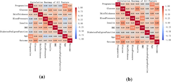
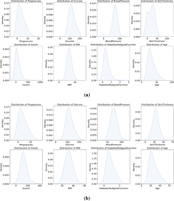
In this experiment, we preprocessed the data, including missing value filling and outlier processing, to improve the accuracy and reliability of data analysis. We used the IQR method to identify and process outliers in the data. As shown in Fig.  4a, it can be clearly seen that some data points deviate from the main data concentration area, and these points are identified as outliers. In order to reduce the impact of these outliers on the analysis results, we replace these outliers with the median of the data. After using the median to fill the outliers, as shown in Fig.  4b, after the median replacement, the data distribution is more concentrated and the impact of extreme values is significantly reduced. This processing step ensures the stability and accuracy of subsequent data analysis and improves the reliability of the results. As shown in Fig. 5 , we can see that after data preprocessing, the correlation between the attributes becomes more significant, and the Pearson correlation coefficient between the independent variables and the dependent variable increases significantly. Through this preprocessing method, we can more accurately reflect the true characteristics of the data, providing a more reliable foundation for subsequent data analysis and model building. Before data preprocessing, as shown in Fig. 6a, some variables have obvious skewness and outliers, especially Glucose, BloodPressure, SkinThickness, BMI and other variables. These skewness and outliers may have an adverse impact on the data analysis results. Therefore, in order to improve the influence of data normality distribution, we need to preprocess the PID dataset. Figure  6b shows the distribution of each variable after data preprocessing. By filling missing values and processing outliers, the distribution of data is closer to normal distribution, and the skewness of features is significantly reduced. For example, the distribution of insulin and skin thickness is smoother, and the impact of outliers on the overall distribution is significantly reduced. Overall, the preprocessed data is more in line with the assumption of normal distribution, which provides a more reliable data basis for subsequent statistical analysis and modeling.

Fig. 4.

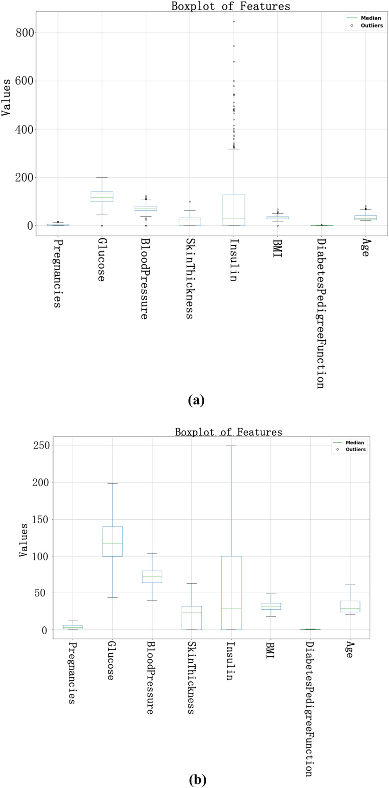
Box plots before and after outlier processing. (a) is the outlier identification result before data preprocessing, and (b) is the outlier identification result after outlier processing.

Fig. 5.

Correlation matrix. (a) is the correlation matrix of variables before data preprocessing. (b) is the correlation matrix of variables after data preprocessing.

Fig. 6.

Data distribution before and after data preprocessing. (a) The number distribution before the calculation, (b) The distribution after the calculation.

Performance evaluation

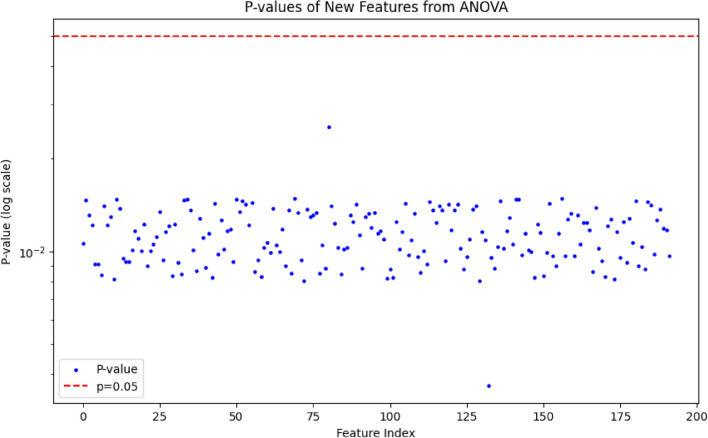
In this experiment, we used the PID dataset for analysis, where each sample contains 8 independent variables. Due to the limited number of features, it was not possible to train an effective model, so we designed an SAE to expand the 8 independent variables in the dataset to 200 variables. Furthermore, we use ANOVA to evaluate the importance of extended features in different categories. As shown in Fig.  7, we ensured that each p-value was less than 0.05 by calculating the p-value of each feature and visualizing it to confirm that the feature significantly contributed to the classification task.

Fig. 7.

Generate feature ANOVA for feature importance of generated features.

The DCTSD-Model proposed in this study uses the Adam optimizer during training, and the learning rate is finally determined to be 0.001 through multiple experiments. The loss function uses the cross-entropy loss. In order to effectively evaluate the performance of the model, 10-fold cross validation is used during training, and weighted sampling is used to deal with the imbalanced category problem to ensure the balance of category distribution. In addition, in order to improve the generalization ability of the student model, KL divergence loss is used for knowledge distillation, and the student model is trained and soft labels are obtained from the teacher model for learning. Similarly, the CNN model also uses a learning rate of 0.001 and a cross-entropy loss function, and performs 10-fold cross validation. All experiments are compared and analyzed on the basis of ensuring the same data preprocessing method.

The proposed CNN and DCTSD-Model are evaluated on the feature-enhanced dataset using 10-fold cross validation. As shown in Table 2, the indicators of the CNN model are significantly improved after using the SAE feature enhancement method. In the DCTSD-Model, we define two teacher models and use a weighted random sampler to give high weights to samples of category 1 and category 0. First, the teacher models are trained for 500 epochs. The teacher models continuously optimize their parameters by minimizing the cross entropy loss function to improve the prediction ability of their respective categories. After the teacher models are trained, we use them to generate soft labels for the training set: the first teacher model is used for category 1 and the second teacher model is used for category 0. These soft labels help the student model learn rich category information. Next, the student model is distilled by minimizing the KL divergence between its output and the soft label, and this process lasts for 500 epochs. In this way, the student model can learn useful knowledge from the teacher model, thereby improving its generalization ability. After distillation training, we fine-tune the student model for 50 epochs using the original labels to ensure that the student model has good prediction ability for the actual labels. In terms of performance improvement, after using the SAE feature enhancement method, the accuracy, recall rate, F1 score and precision of CNN increased by 3.48%, 3.45%, 3.47% and 3.45% respectively compared with before feature enhancement. The accuracy of DCTSD-Model reached 98.58%, and as shown in Fig.  8, DCTSD-Model has a significant improvement in AUC compared to CNN. Compared with CNN, the precision, recall, F1 score, accuracy and AUC increased by 3.48%, 3.45%, 3.47%, 3.45% and 5.47% respectively.

Table 2.

Model performance for prediction.

Model	Precision (%)	Recall (%)	F1-Score (%)	Accuracy (%)	AUC (%)
CNN	94.15	94.18	94.16	94.18	93.36
SAE+CNN	95.11	95.13	95.12	95.13	93.65
SAE+DCTSD-Model	98.59	98.58	98.59	98.58	99.12

Fig. 8.

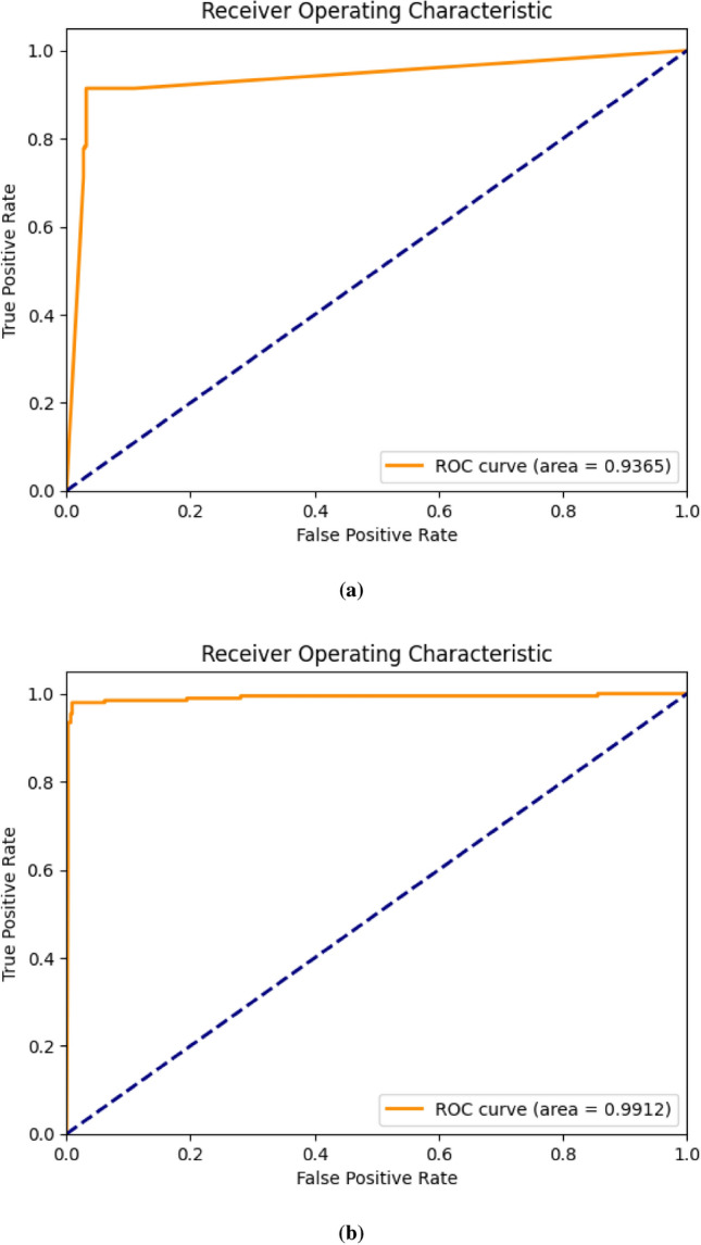
ROC curve diagram. (a) is the ROC curve of CNN, and (b) is the ROC curve of DCTSD-Model.

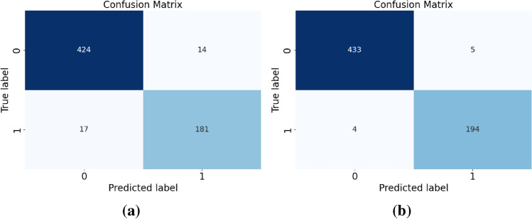
Figure 9a and b show the confusion matrix results. CNN has 14 and 17 misclassifications when predicting category 0 and category 1, respectively, while DCTSD-Model has only 5 and 4 misclassifications. Specifically, CNN correctly predicted 424 samples and incorrectly predicted 14 samples when predicting category 0; correctly predicted 181 samples and incorrectly predicted 17 samples when predicting category 1. However, DCTSD-Model correctly predicted 433 samples and incorrectly predicted 5 samples when predicting category 0; correctly predicted 194 samples and incorrectly predicted 4 samples when predicting category 1. It is obvious that the enhanced model performs better in reducing the number of misclassifications.

Fig. 9.

Confusion matrix. (a) is the confusion matrix of CNN, and (b) is the confusion matrix of DCTSD-Model.

Overall, the SAE and DCTSD-Model feature enhancement methods significantly improved the classification performance of the model, making it show higher accuracy and reliability in various evaluation indicators. These experimental results show that the performance of the DCTSD-Model proposed in this study in classification tasks has been significantly improved. The accuracy shows the proportion of correct classifications of the model, the ROC curve and AUC value show the classification ability of the model at different thresholds, and the confusion matrix shows the prediction of each category in detail. Overall, the new knowledge distillation process proposed in this study effectively improves the classification performance and generalization ability of the student model. The effectiveness and superiority of this method in practical applications provide a solid foundation for further research and application.

Discussion

Diabetes prediction is an important research topic in healthcare. Accurate prediction helps early intervention and reduces patient risks and medical costs. In this study, we proposed a new method for feature enhancement using SAE and classification using DCTSD-Model for PID dataset, aiming to improve the accuracy and reliability of diabetes prediction.CNN as the base model in this model has advantages in diabetes classification, but due to the low feature dimension of the PID dataset, it is not enough to train an efficient model. Therefore, we use SAE to expand the variables of the original data and enhance the feature expression ability. Experimental results show that after SAE feature enhancement, the indicators of the CNN model are significantly improved. DCTSD-Model adopts a dual teacher model and knowledge distillation method to help the student model learn rich category information by generating soft labels, and uses a weighted random sampler to deal with the category imbalance problem.

In this study, the DCTSD-Model we proposed showed significant advantages in classification performance. Table 3 shows the research results of relevant literature in this field in the past three years. The accuracy of different models in diabetes prediction varies, ranging from 89% to 98%. Compared with other methods, DCTSD-Model has significant advantages. First, DCTSD-Model has an accuracy of 98.57%, which is significantly higher than other methods. This means that the model has a higher classification accuracy in the diabetes prediction task and can more accurately identify individuals with diabetes.

Table 3.

Literature comparison.

Model	Accuracy (%)	Related literature	Date
ANN	93.00	Bukhari et al.15	2021
2GDNN	97.25	Olisah et al.13	2022
FMDP	94.87	Ahmed et al.17	2022
DPMBFSEL	98.00	Zhou et al.19	2023
Super Learner Model (LR, DT, RF, GB)	92.00	Doğru et al.16	2023
XGBoost	89.00	Alghamdi et al.20	2023
SECNN	89.47	Zhao et al.16	2024
XGBoost	95.40	Modak et al.30	2024
XGBoost algorithm with SMOTE	97.40	El-Sofany et al.31	2024
DCTSD-Model	98.57	This study	–

Among them, the PID dataset uses SAE to expand the 8 independent variables of the original data to 200 variables, which greatly enhances the expressiveness of the features and captures more potential information. In addition, DCTSD-Model uses a dual teacher model and knowledge distillation method to train the data of category 0 and category 1 through two teacher models respectively, and generate soft labels to help the student model learn rich category information, further improving the generalization ability of the model.This method also effectively handles the problem of category imbalance by assigning different weights to data of different categories, so that the model can better learn the characteristics of each category during training.

In future studies, we can explore more efficient feature enhancement methods and distillation strategies to further improve the performance and applicability of the diabetes classification model. In addition, we can also consider testing the model on more diverse datasets to verify its wide application potential.

Conclusion

This study proposed a diabetes prediction model DCTSD-Model based on a new knowledge distillation. The PID dataset was preprocessed and a SAE method for feature enhancement was established. This method significantly improved the classification performance of the model. Feature enhancement through SAE greatly enhanced the expressive power of the features. DCTSD-Model uses a dual teacher model and knowledge distillation method to help the student model learn rich category information by generating soft labels and effectively handle the category imbalance problem. Experimental results show that the accuracy of DCTSD-Model reaches 98.57%, showing excellent performance in processing diabetes prediction tasks.

The results of this study provide an effective solution for diabetes prediction and lay a solid foundation for future research and application. Further research can explore more diverse data sets and application scenarios, verify the wide applicability of the model, and continue to optimize feature enhancement and knowledge distillation methods to further improve the performance and efficiency of the model.

Author contributions

H.G. and J.Z. conceived the experimental methods, L.S., H.W., and Z.D. collected and processed the experimental data, H.G. conducted the experiments, H.G. and Z.K. analyzed and visualized the results. H.G. wrote the manuscript. All authors reviewed the manuscript. All authors gave their permission for the publication of the final version of the manuscript.

Data availability

This study analyzed an openly available dataset. The dataset can be downloaded at https://www.kaggle.com/.

Declarations

Competing interests

The authors declare no competing interests.

References

- 1.Mealey, B. L. & Oates, T. W. Diabetes mellitus and periodontal diseases. J. Periodontol.77, 1289–1303 (2006). [DOI] [PubMed] [Google Scholar]
- 2.Katsarou, A. et al. Type 1 diabetes mellitus. Nat. Rev. Dis. Primers3, 1–17 (2017). [DOI] [PubMed] [Google Scholar]
- 3.DeFronzo, R. A. et al. Type 2 diabetes mellitus. Nat. Rev. Dis. Primers1, 1–22 (2015). [DOI] [PubMed] [Google Scholar]
- 4.Dabelea, D. et al. Increasing prevalence of gestational diabetes mellitus (gdm) over time and by birth cohort: Kaiser permanente of colorado gdm screening program. Diabet. care28, 579–584 (2005). [DOI] [PubMed] [Google Scholar]
- 5.Kaur, R., Kaur, M. & Singh, J. Endothelial dysfunction and platelet hyperactivity in type 2 diabetes mellitus: Molecular insights and therapeutic strategies. Cardiovasc. Diabetol.17, 1–17 (2018). [DOI] [PMC free article] [PubMed] [Google Scholar]
- 6.Bailey, C. J. & Day, C. Treatment of type 2 diabetes: Future approaches. Br. Med. Bull.126, 123–137 (2018). [DOI] [PubMed] [Google Scholar]
- 7.Lebovitz, H. E. Type 2 diabetes: An overview. Clin. Chem.45, 1339–1345 (1999). [PubMed] [Google Scholar]
- 8.Stumvoll, M., Goldstein, B. J. & Van Haeften, T. W. Type 2 diabetes: Principles of pathogenesis and therapy. The Lancet365, 1333–1346 (2005). [DOI] [PubMed] [Google Scholar]
- 9.Chatterjee, S., Khunti, K. & Davies, M. J. Type 2 diabetes. The Lancet389, 2239–2251 (2017). [DOI] [PubMed] [Google Scholar]
- 10.Safiri, S. et al. Prevalence, deaths and disability-adjusted-life-years (dalys) due to type 2 diabetes and its attributable risk factors in 204 countries and territories, 1990–2019: results from the global burden of disease study 2019. Front. Endocrinol.13, 838027 (2022). [DOI] [PMC free article] [PubMed] [Google Scholar]
- 11.Hasan, M. K., Alam, M. A., Das, D., Hossain, E. & Hasan, M. Diabetes prediction using ensembling of different machine learning classifiers. IEEE Access8, 76516–76531 (2020). [Google Scholar]
- 12.Khanam, J. J. & Foo, S. Y. A comparison of machine learning algorithms for diabetes prediction. Ict Express7, 432–439 (2021). [Google Scholar]
- 13.Olisah, C. C., Smith, L. & Smith, M. Diabetes mellitus prediction and diagnosis from a data preprocessing and machine learning perspective. Comput. Methods Progr. Biomed.220, 106773 (2022). [DOI] [PubMed] [Google Scholar]
- 14.Ahmed, U. et al. Prediction of diabetes empowered with fused machine learning. IEEE Access10, 8529–8538 (2022). [Google Scholar]
- 15.Zhou, H., Xin, Y. & Li, S. A diabetes prediction model based on Boruta feature selection and ensemble learning. BMC Bioinform.24, 224 (2023). [DOI] [PMC free article] [PubMed] [Google Scholar]
- 16.Doğru, A., Buyrukoğlu, S. & Arı, M. A hybrid super ensemble learning model for the early-stage prediction of diabetes risk. Med. Biol. Eng. Comput.61, 785–797 (2023). [DOI] [PubMed] [Google Scholar]
- 17.Alghamdi, T. Prediction of diabetes complications using computational intelligence techniques. Appl. Sci.13, 3030 (2023). [Google Scholar]
- 18.García-Ordás, M. T., Benavides, C., Benítez-Andrades, J. A., Alaiz-Moretón, H. & García-Rodríguez, I. Diabetes detection using deep learning techniques with oversampling and feature augmentation. Comput. Methods Progr. Biomed.202, 105968 (2021). [DOI] [PubMed] [Google Scholar]
- 19.Bukhari, M. M. et al. An improved artificial neural network model for effective diabetes prediction. Complexity2021, 5525271 (2021). [Google Scholar]
- 20.Zhao, J. et al. Attention-oriented cnn method for type 2 diabetes prediction. Appl. Sci.14, 3989 (2024). [Google Scholar]
- 21.Kaiser, J. Dealing with missing values in data. J. Syst. Integr. (1804-2724)5 (2014).
- 22.Dixon, W. Processing data for outliers. Biometrics9, 74–89 (1953). [Google Scholar]
- 23.Vinutha, H., Poornima, B. & Sagar, B. Detection of outliers using interquartile range technique from intrusion dataset. In Information and decision sciences: Proceedings of the 6th international conference on ficta, 511–518 (Springer, 2018).
- 24.Shanker, M., Hu, M. Y. & Hung, M. S. Effect of data standardization on neural network training. Omega24, 385–397 (1996). [Google Scholar]
- 25.Ng, A. et al. Sparse autoencoder. CS294A Lecture notes72, 1–19 (2011).
- 26.Gou, J., Yu, B., Maybank, S. J. & Tao, D. Knowledge distillation: A survey. Int. J. Comput. Vis.129, 1789–1819 (2021). [Google Scholar]
- 27.Hinton, G., Vinyals, O. & Dean, J. Distilling the knowledge in a neural network. arXiv preprint arXiv:1503.02531 (2015).
- 28.Wong, T.-T. & Yeh, P.-Y. Reliable accuracy estimates from k-fold cross validation. IEEE Trans. Knowl. Data Eng.32, 1586–1594 (2019). [Google Scholar]
- 29.Lobo, J. M., Jiménez-Valverde, A. & Real, R. Auc: A misleading measure of the performance of predictive distribution models. Glob. Ecol. Biogeogr.17, 145–151 (2008). [Google Scholar]
- 30.Modak, S. K. S. & Jha, V. K. Diabetes prediction model using machine learning techniques. Multim. Tools Appl.83, 38523–38549 (2024). [Google Scholar]
- 31.El-Sofany, H., El-Seoud, S. A., Karam, O. H., Abd El-Latif, Y. M. & Taj-Eddin, I. A. A proposed technique using machine learning for the prediction of diabetes disease through a mobile app. Int. J. Intell. Syst.2024, 6688934 (2024). [Google Scholar]
Associated Data
This section collects any data citations, data availability statements, or supplementary materials included in this article.
Data Availability Statement