Abstract
Precise estimation of rock petrophysical parameters are seriously important for the reliable computation of hydrocarbon in place in the underground formations. Therefore, accurately estimation rock saturation exponent is necessary in this regard. In this communication, we aim to develop intelligent data-driven models of decision tree, random forest, ensemble learning, adaptive boosting, support vector machine and multilayer perceptron artificial neural network to predict rock saturation exponent parameter in terms of rock absolute permeability, porosity, resistivity index, true resistivity, and water saturation based on acquired 1041 field data. A well-known outlier detection algorithm is applied on the gathered data to assess the data reliability before model development. Additionally, relevancy factor is estimated for each input parameter to assess the relative effects of input parameters on the saturation exponent. The sensitivity analysis indicates that resistivity index and true resistivity have direct correlation with the saturation exponent while porosity, absolute permeability and water saturation is inversely related with saturation exponent. In addition, the graphical-based and statistical-based evaluations illustrate that AdaBoost and ensemble learning models outperforms all other developed data-driven intelligent models as these two models are associated with lowest values of mean square error (adaptive boosting: 0.017 and ensemble learning: 0.021 based on unseen test data) and largest values of coefficient of determination (adaptive boosting: 0.986 and ensemble learning: 0.983 based on unseen test data).
Keywords: Saturation exponent, Data-driven intelligent modeling, Sensitivity analysis, Outlier detection
Subject terms: Carbon capture and storage, Fossil fuels, Energy infrastructure, Solid Earth sciences
Introduction
The primary goal of an engineered petrophysical program within the realm of petroleum industry is to evaluate the quantity of hydrocarbons1. Although Archie’s parameters of m, a and n are generally assumed constant in standard formations, the saturation exponent (n) can vary significantly, ranging often from 20 to 2 in formations that are strongly oil-wet to water-wet under specific conditions. Numerous study outcomes contend that the parameter of saturation exponent is highly influenced by wettability, displacement history, and pore size distribution, with values potentially ranging from 2 to 102,3. Traditionally, the cementation exponent (m) in Archie’s equation has been the focus of extensive studies and research. With the advent of the Pickett Plot method for estimating m using wireline measurements method of porosity and resistivity, it can now be computed through crossplotting. In contrast, the saturation exponent (n) and tortuosity factor (a) are generally left unaltered, except in cases where core measurements suggest a deviation from the typical value, such as n = 24,5. In the world of petrophysics, it is essential to acquire accurate Archie’s parameters’ values to specify the exact water saturation of underground reservoir formations3,6–8. Assuming a constant saturation exponent, particularly in formations with diverse rock types, should be considered a last resort. The conventional approach to calculating the saturation exponent involves obtaining experimental data through special core analysis, which straightly yields Archie’s parameters. However, the primary drawback of such methods is the associated cost and time required for the pertinent experiments3,9,10.
The literature presents numerous studies over the specification of the saturation exponent. Al-Hilali4 proposed a straightforward petrophysics-based workflow for rigorously estimating the water saturation exponent. Godarzi et al.11 introduced two innovative techniques of MGA (Modified Genetic Algorithm) and HDP (Homogeneous Distribution of Parameters) for simultaneously determining the parameters of Archie’s equation, and associated these methods with traditionally-existing approaches. Hamada12 developed a novel practice for calculating Archie’s equation factors, utilizing a 3D plot that incorporates formation porosity, water saturation, and formation water resistivity. A comparative analysis of the accuracy of each separate method was also illustrated. Mardi et al.13 proposed an artificial neural network based method to determine the cementation factor, saturation exponent, and water saturation.
Recently, innovative methods based on soft computing have been successfully introduced and extensively applied in the fields of chemical, earth sciences, mining engineering and petroleum engineering14–16. These methods are significantly more robust than classical regression and traditional statistical techniques in deriving input/output data relationships17. For example, a primary scheme is the application of artificial neural networks (ANNs) for classification and highly non-linear regression problems, which is well-regarded for its rapid estimation and strong generalization capabilities following effective network training15. Another soft computing approach involves the recent development of a robust technique known as Support Vector Machine (SVM), which incorporates its associated learning algorithm for data analysis and pattern recognition18. SVM has garnered significant consideration for its exceptional functioning in addressing complex regression problems and classification19. SVM has been extensively applied across engineering and scientific disciplines, including the prediction of permeability and porosity based on well log data and lithology, as well as in speech and text recognition, and pattern identification in medical science20–23.
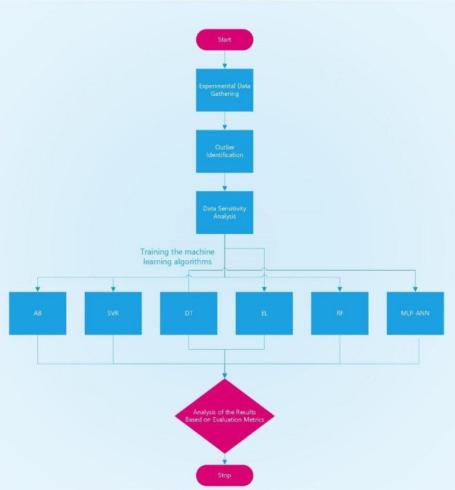
In this study, an initial sensitivity analysis is conducted to identify the sensitive parameters using the relevancy factor, followed by outlier detection to learn about the reliability of the data required for the data-driven modeling process based upon 1041 gathered field data. Then, robust machine learning methods of Decision Tree (DT), AdaBoost (AB), Random Forest (RF), Ensemble Learning (EL), Convolutional Neural Network (CNN), Support Vector Machine (SVM) and Multilayer Perceptron Artificial Neural Network (MLP-ANN) are used to create highly robust, accurate and intelligent data-driven models to predict saturation exponent of underground petroleum reservoir formations in terms of absolute permeability, porosity, true resistivity, water saturation, and resistivity index in an easy and user-friendly way based on acquired field data. The constructed models are evaluated and assessed using several statistical indices and graphical approaches. The step-by-step workflow as a flowchart is given in Fig. 1. Notice that Each algorithm brings unique strengths to the workflow: for instance, Decision Trees and Random Forests are well-suited for interpretability and handle categorical variables effectively, while CNNs and MLP-ANNs are powerful in capturing complex, nonlinear patterns. By using an ensemble approach, we can enhance predictive accuracy and robustness, as it allows us to leverage the combined strengths of individual models. However, there are limitations to each method. For instance, Decision Trees can overfit without proper pruning and while neural networks such as CNNs and MLP-ANNs can uncover intricate relationships, they are computationally intensive and can be challenging to interpret. Additionally, some algorithms like SVM are sensitive to parameter tuning, which can affect their performance24.
Fig. 1.
Step-by-step workflow followed in this paper for the intelligent modeling of rock saturation exponent.
Modeling background and methodology
Modeling background
In this part, the description of each machine learning algorithm utilized in the current study is put forward.
Decision tree
Decision Trees represent a powerful suite of machine learning algorithms designed for classification and regression tasks25. Developed to categorize and make predictions on previously unseen data, the Decision Tree algorithm works by building a tree-like structure that recursively splits the dataset, driven by the feature that yields the highest information gain or reduction in impurity, until a pre-defined stopping criterion is met. This process culminates in a tree with leaf nodes representing the majority class or prediction for new samples. More technical descriptions along with the pertaining equations may be found in26.
AdaBoost
AdaBoost27 (Adaptive Boosting) is a widely-used ensemble technique that combines multiple weak learners, referred to as base estimators, to form a more powerful and accurate regressor for prediction tasks. The AdaBoost algorithm commences by fitting a base estimator to the raw data, after which it proceeds to fit additional copies of the same estimator to the data with adjusted instance weights that depend on the current prediction errors. This iterative process ultimately yields a weighted combination of the base estimators, which together constitute the boosted regressor, resulting in improved predictive accuracy28.
Random Forest
The Random Forest regressor is a robust ensemble learning methodology that leverages multiple decision trees to enhance the accuracy and generalizability of the resulting model. By combining the predictions of numerous individual trees, each trained on a random subset of the data and features, the Random Forest algorithm effectively reduces overfitting and captures the underlying patterns within the data. This powerful approach to regression tasks not only yields accurate predictions but also enables the assessment of feature importance, providing valuable insights into the factors that contribute most significantly to the observed outcomes29. The Random Forest algorithm has garnered substantial popularity within the machine learning domain due to its ability to deliver strong performance without requiring extensive hyperparameter tuning. Furthermore, its capacity to handle large-scale datasets makes it an attractive choice for real-world applications where data abundance can be overwhelming for other algorithms. This combination of robustness, ease of use, and scalability contributes to the widespread adoption of Random Forests as a go-to method for various classification and regression tasks across diverse domains30.
Ensemble learning
Ensemble learning techniques generate a collective decision-making process by amalgamating the powers of individual learning models to achieve improved reliability. These methodologies can be characterized into non-generative and generative approaches, depending on their prediction generation strategy. Non-generative ensemble learning techniques focus on producing new predictions by integrating the outputs of independently trained models, without intervening in their learning stages. Conversely, generative ensemble learning techniques have the capability to construct the underlying learners, while also optimizing learning algorithms and datasets within the ensemble. Among non-generative ensemble learning methods, the voting ensemble and stacking ensemble techniques are the most prominent. The voting ensemble regression method calculates a final prediction by averaging the predictive outcomes of combined independent learning algorithms, thus leveraging the strengths of multiple models for enhanced predictive performance31.
Support vector machine
The kernel function within the support vector machine (SVM) is responsible for mapping sample data into high-dimensional space enabling the solution of nonlinear regression problems32. To ensure SVM predictive model is associated with generalization capability and prediction accuracy, parameter optimization selection, kernel function and sample data processing are the key components that needs to be delicately taken into account. In this regard, the mapping relationship between the output variable and input variables is expressed as:
 |
1 |
In which y is the output variable and x being the input variable and n represents the number of input variables. Kernel function determines the predictive performance of SVM model. The most commonly used kernel function is called radial basis function (RBF), the details of which can be found in33.
Multilayer perceptron artificial neural network
Artificial Neural Networks (ANNs) are powerful mathematical tools that draw inspiration from the structure and function of the human nervous system. As noted previously, the foundation of ANNs lies in mimicking the human brain’s parallel processing capabilities for uncovering intricate nonlinear relationships between independent and dependent variables. By employing interconnected layers of artificial neurons, ANNs can learn from data, adapt to new inputs, and generate accurate predictions in complex problem domains34. ANNs represent sophisticated statistical tools that emulate the human nervous system’s interconnected neurons within a computational network. ANNs encompass various types and architectures, each tailored to specific tasks and problem domains. These models excel at pattern recognition and decision-making, with applications spanning numerous scientific fields. The extensive adoption of ANNs across diverse disciplines highlights their versatility and efficacy in addressing complex challenges, positioning them as a prominent tool in contemporary scientific research35,36. The remarkable precision of ANNs positions them as highly effective nonlinear analysis tools, capable of replacing time-consuming and costly experimental procedures. ANNs have demonstrated their ability to address intricate modeling tasks, including prediction, pattern recognition, and classification, establishing their prominence in scientific research37.
Methodology
Gathered data statistics
The dataset employed in this research comprises field data with 1041 datapoints of routine and special core analysis (RCAL and SCAL) as functions of absolute permeability, porosity, true resistivity, water saturation and resistivity index. The statistical properties of these data are outlined in Table 1. It is well-established within the field of petrophysics which involves geological formation properties, the rock saturation exponent is linked to above-mentioned specifications, albeit with varying degrees of correlation and directionality. Given these relationships, the input parameters used for the data-driven model development encompass absolute permeability, porosity, true resistivity, water saturation, and resistivity index as the required input factors. The output label is the saturation exponent.
Table 1.
Statistical values of the gathered field dataset for the data-driven model development in this study.
| Parameter | Minimum | Maximum | Mean |
|---|---|---|---|
| Porosity, % | 1.26 | 32.13 | 14.73 |
| Absolute permeability, mD | 0.03 | 4479.56 | 190.72 |
| Water saturation, dimensionless | 0.06 | 1.01 | 0.63 |
| True resistivity, ohm.m | 0.37 | 2495.05 | 53.25 |
| Resistivity index, ohm.m | 0.39 | 360 | 8.28 |
| Saturation exponent, dimensionless | 0.00 | 7.80 | 1.60 |
Sensitivity analysis
In this part, we seek to find out the relative effect of each input variable including absolute permeability, porosity, true resistivity, water saturation and resistivity index on the output factor which is saturation exponent. This is carried out here with the consideration of relevancy factor in which it is calculated for each separate input variable. The equation of relevancy factor is defined as38:
 |
2 |
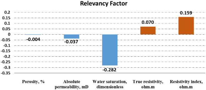
In which j denotes the specific input variable. Note that the probable range of relevancy factor lies within -1 and + 1. Also, the higher the magnitude of the calculated relevancy factor, the stronger the relationship of the specific input variable with the output variable. In addition, a negative and positive relevancy index indicate indirect and direct relationship of the so-called input variable with pertinent output variable. In this way, the estimated relevancy factor for all the considered input factors is given in Fig. 2. As can be seen, resistivity index and true resistivity are directly correlated with saturation exponent while porosity, absolute permeability and water saturation is inversely related with saturation exponent. Additionally, water saturation has the strongest relationship with output variable.
Fig. 2.
Exploring the relative impact of each variable on the saturation exponent using relevancy factor.
Outlier detection
The reliability of any data-driven intelligent model is significantly influenced by the quality of the dataset employed during the development process. To ensure the credibility of the data in this study, we apply the widely recognized Leverage technique, which involves the utilization of the Hat matrix. This matrix is defined as follows38:
 |
3 |
In the aforementioned equation, the design matrix X is denoted as an m*n matrix, where n signifies the number of input variables and m represents the total number of data points. To identify potential outliers using the Leverage technique, we employ the Williams’ plot, which visualizes the relationship between the Hat values and their normalized counterparts. Within this graphical representation, the warning leverage is determined through the following calculation38:
 |
4 |
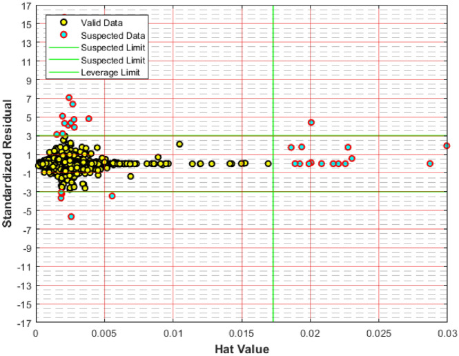
It is important to note that standardized residuals typically fall within the range of -3 to + 3. The Williams’ plot, presented in Fig. 3, facilitates the identification of outlier and suspect data points. The plot features two horizontal lines representing standardized residual values, and a vertical line indicating the warning leverage value. Data points located within these boundaries are deemed reliable and validated. As illustrated in Fig. 3, only 26 out of 1401 datapoints are classified as outliers. Despite this, all datapoints are taken into account during model development to ensure the construction of generalized models.
Fig. 3.
Identification of suspected data before intelligent data-driven modeling via Leverage methodology.
Model evaluation indices
In order to comprehend the robustness, reliability and accuracy of the developed models, the following statistical indices are estimated for each model39–41:
 |
5 |
 |
6 |
 |
7 |
 |
8 |
Wherein exp and pre are known as field and estimated values, i denotes index number and the number of datapoints are depicted via N.
The input variables for the data-driven modeling include absolute permeability, porosity, true resistivity, water saturation and resistivity index for the modeling process of saturation exponent. Moreover, 80%, 10% and 10% of all datapoints are randomly selected for training, validation and testing phases, respectively. As widely known, the validation is used to avoid overfitting while testing is implemented using the unseen data during the model training (development) phase. To minimize the impact of data fluctuations during the modeling process, both input and output variables are normalized using the following relationship:
 |
9 |
Where the real value is denoted by n, subscripts max and min signify maximum and minimum value of the dataset and subscript norm is known as the normalized value.
Results and discussion
Determination of optimum parameters
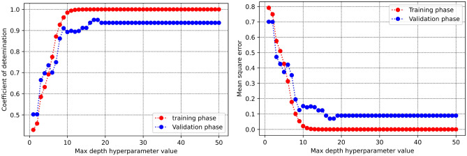
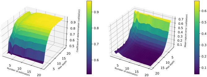
In this part, the process of obtaining the hyperparameters are discussed. Figure 4 displays coefficient of determination and mean square error versus maximum depth hyperparameter within the decision tree approach. As can be seen, the optimum value is calculated to be 17. The same value (that is, 17) is estimated as the optimum value of number of estimators as the hyperparameter within the AdaBoost machine learning method as demonstrated in Fig. 5. Figure 6 represents two 3D plots of mean square error and determination coefficient of the validation phase in random forest approach. As seen, the optimum values of maximum depth and number estimators are 14 and 16 respectively. Additionally, the optimized value of SVM hyperparameter (c) is estimated to be 461 as can be observed in Fig. 7. The process of MLP-ANN in terms of mean square error versus iteration for training and validation phases is indicated in Fig. 8. Notice that the tuned specifications of all the trained machine learning algorithms in this study are tabulated in Table 2.
Fig. 4.
Determination of max depth hyperparameter optimum value in Decision Tree method.
Fig. 5.
Determination of number of estimators’ hyperparameter optimum value in AdaBoost method.
Fig. 6.
Determination of optimum parameters (number of estimators and max depth) in Random Forest approach.
Fig. 7.
Determination of optimum hyperparameter (c) in the SVM approach.
Fig. 8.
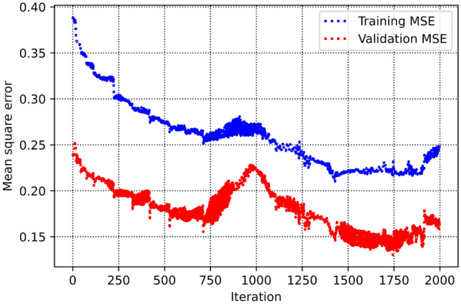
MSE versus iteration in the process of implementation of MLP-ANN approach.
Table 2.
Key tuned specifications for all the trained machine learning algorithms in this study.
| Utilized machine learning algorithm | Key tuned specifications |
|---|---|
| Decision Tree | • Max depth: 17 |
| Random Forest |
• Max depth: 14 • Number of estimators: 16 |
| Adaptive Boosting |
• Number of estimators: 17 • Learning Rate = 1.0 |
| Ensemble Learning | • Base estimators: Decision Tree, Random Forest, and Adaptive Boosting (all with their tuned specifications) |
| Support Vector Machine |
• Kernel function: Radial Basis Function (RBF) • Gamma type: Scaled • C hyperparameter: 461 |
| Multilayer Perceptron Artificial Neural Network |
• Activation function: ReLU (Rectified Linear Unit) • Learning rate = 0.001 • Number of hidden layers: 8 • Number of neurons within in hidden layer: 13 |
Models’ evaluation
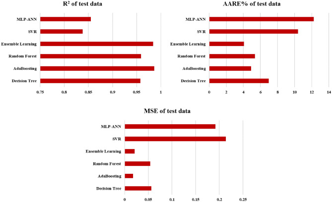
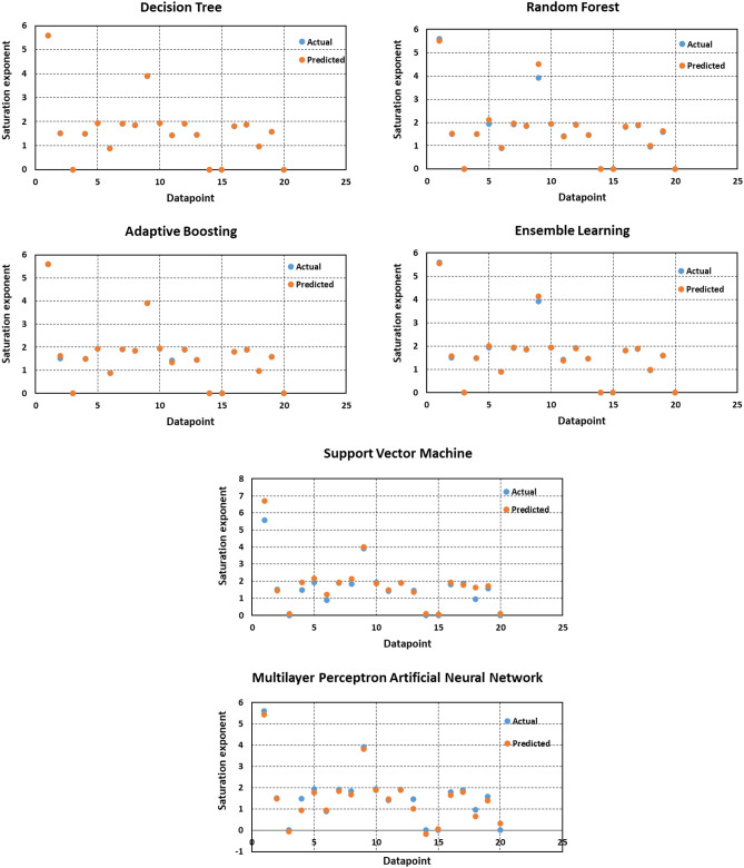
Table 2 tabulates the evaluation indices of coefficient determination, mean square error and average absolute relative error (AARE%) for the developed data-driven intelligent models of decision tree, AdaBoost, random forest, ensemble learning, support vector machine and multilayer perceptron artificial neural network. In addition, for better doing the evaluation task, these parameters for the testing phase are depicted in Fig. 9. Moreover, Table 3 tabulates predicted values for 20 random data via the trained algorithms.
Fig. 9.
Mean square error, coefficient of determination and average absolute relative error percent for the test phase for all the approaches.
Table 3.
Obtained evaluation statistical indices for all the developed data-driven methods for training, validation and test phases as well as total data.
| Model | R2 | MSE | AARE% | |||||||||
|---|---|---|---|---|---|---|---|---|---|---|---|---|
| Training | Validation | Test | Total | Training | Validation | Test | Total | Training | Validation | Test | Total | |
| DT | 0.999999 | 0.9503637 | 0.957304 | 0.990473 | 9.81E-07 | 0.069887 | 0.056359 | 0.013272 | 0.005422 | 8.6386931 | 6.9581152 | 2.003791 |
| AB | 0.999591 | 0.9747454 | 0.986566 | 0.995646 | 0.000567 | 0.0355581 | 0.017733 | 0.006097 | 0.552514 | 6.698052 | 4.9120449 | 2.022674 |
| RF | 0.984169 | 0.9641713 | 0.958918 | 0.980752 | 0.021959 | 0.0504462 | 0.054228 | 0.028306 | 4.95995 | 17.991411 | 5.3604011 | 7.815577 |
| EL | 0.99821 | 0.974859 | 0.983977 | 0.99454 | 0.002483 | 0.035398 | 0.021151 | 0.007939 | 1.882193 | 10.162351 | 4.07001 | 3.65743 |
| SVR | 0.749724 | 0.8293293 | 0.838151 | 0.771682 | 0.347161 | 0.2403014 | 0.213641 | 0.322094 | 15.58514 | 14.346958 | 10.395688 | 15.18521 |
| MLP-ANN | 0.820927 | 0.8829975 | 0.854825 | 0.843533 | 0.248395 | 0.1647375 | 0.191631 | 0.233589 | 18.28915 | 25.900553 | 12.227834 | 19.5458 |
As can be seen, the AdaBoost and ensemble learning methods have the lowest mean square error and AARE%, which means they have the best performance in predicting saturation exponent. In addition, these methods have accordingly the highest values of determination coefficient. For the prediction of saturation exponent in this paper, it appears that MLP-ANN and SVR are less accurate as they have the highest values of MSE and AARE% while they have the lowest values of determination coefficient.
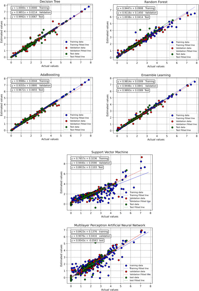
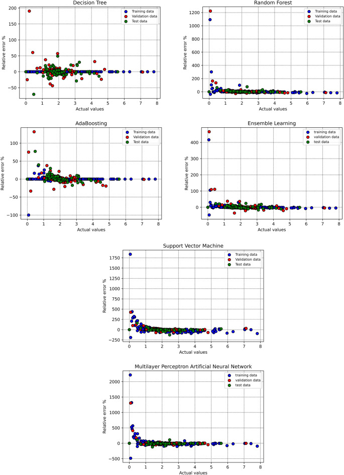
To assess the performance of the trained algorithms and analyze their estimation accuracy, several visual plots are employed in this study. First, cross plots are generated for all proposed models, as shown in Fig. 10. For both AdaBoost and ensemble learning models, the clustering of points around the unit slope line indicates a high degree of accuracy. Furthermore, the equations obtained from fitting lines on these points are remarkably close to the bisector line. Also, the distribution of relative deviation for each estimator is illustrated in Fig. 11. A closer proximity of the data to the y = 0 line corresponds to higher estimator accuracy. According to this plot, the AdaBoost and ensemble learning models emerge as the most effective predictive tools. Figure 12 also depicts the crossplots of estimated versus actual datapoints tabulated in Table 4 which includes 20 random datapoints taken from all the dataset.
Fig. 10.
Crossplots of estimated versus real values for all the developed intelligent models per training, validation and test phases in this study.
Fig. 11.
Distribution of relative error based on training, validation and test phases for all the developed data-driven models in this study.
Fig. 12.
Crossplots of estimated versus actual points for the 20 random datapoints tabulated in Table 4.
Table 4.
Comparison of modeling results with the target values for 20 random data.
| Input Parameter | Target Parameter | Target Parameter Predicted by the Trained Algorithm | |||||||||
|---|---|---|---|---|---|---|---|---|---|---|---|
| Porosity (%) | Absolute permeability (md) | Water saturation (fraction) | True resistivity (ohm.m) | Resistivity index (ohm.m) | Saturation exponent (dimensionless) | DT | AB | RF | EL | SVR | MLP-ANN |
| 17.05 | 0.30 | 0.67 | 16.49 | 9.77 | 5.59 | 5.59 | 5.59 | 5.50 | 5.55 | 6.70 | 5.43 |
| 13.60 | 3.30 | 0.56 | 6.09 | 2.40 | 1.51 | 1.51 | 1.62 | 1.53 | 1.56 | 1.44 | 1.49 |
| 15.00 | 5.50 | 1.00 | 1.87 | 1.00 | 0.00 | 0.00 | 0.00 | 0.00 | 0.00 | 0.10 | -0.06 |
| 11.29 | 0.72 | 0.81 | 2.36 | 1.37 | 1.49 | 1.49 | 1.49 | 1.49 | 1.49 | 1.93 | 0.93 |
| 15.90 | 1.56 | 0.85 | 2.91 | 1.38 | 1.94 | 1.94 | 1.94 | 2.12 | 2.01 | 2.18 | 1.78 |
| 15.02 | 1.32 | 0.94 | 3.02 | 1.05 | 0.89 | 0.89 | 0.89 | 0.92 | 0.90 | 1.23 | 0.93 |
| 14.90 | 5.70 | 0.38 | 12.65 | 6.53 | 1.91 | 1.91 | 1.91 | 1.95 | 1.93 | 1.94 | 1.83 |
| 16.50 | 7.00 | 0.78 | 3.70 | 1.57 | 1.85 | 1.85 | 1.85 | 1.85 | 1.85 | 2.13 | 1.68 |
| 7.52 | 12.65 | 0.55 | 127.14 | 10.37 | 3.91 | 3.91 | 3.91 | 4.50 | 4.14 | 4.01 | 3.82 |
| 20.10 | 8.50 | 0.61 | 3.54 | 2.62 | 1.93 | 1.93 | 1.95 | 1.93 | 1.93 | 1.86 | 1.88 |
| 32.13 | 3311.25 | 0.11 | 229.06 | 23.00 | 1.42 | 1.42 | 1.34 | 1.39 | 1.37 | 1.49 | 1.46 |
| 15.64 | 10.12 | 0.69 | 4.26 | 2.05 | 1.91 | 1.91 | 1.89 | 1.90 | 1.90 | 1.89 | 1.90 |
| 3.09 | 0.52 | 0.33 | 2495.05 | 4.97 | 1.46 | 1.46 | 1.46 | 1.46 | 1.46 | 1.36 | 1.00 |
| 10.01 | 2.78 | 1.00 | 22.98 | 1.00 | 0.00 | 0.00 | 0.00 | 0.00 | 0.00 | 0.10 | -0.17 |
| 22.40 | 112.00 | 1.00 | 0.95 | 1.00 | 0.00 | 0.00 | 0.00 | 0.00 | 0.00 | 0.06 | 0.05 |
| 8.43 | 8.86 | 0.37 | 14.10 | 5.96 | 1.80 | 1.80 | 1.80 | 1.83 | 1.81 | 1.92 | 1.66 |
| 7.90 | 0.05 | 0.58 | 33.65 | 2.78 | 1.88 | 1.88 | 1.88 | 1.90 | 1.89 | 1.78 | 1.80 |
| 16.89 | 16.70 | 0.76 | 2.86 | 1.30 | 0.96 | 0.96 | 0.96 | 0.99 | 0.97 | 1.64 | 0.65 |
| 13.40 | 2.20 | 0.72 | 3.75 | 1.70 | 1.58 | 1.58 | 1.58 | 1.62 | 1.60 | 1.72 | 1.38 |
| 3.09 | 0.52 | 1.00 | 502.43 | 1.00 | 0.00 | 0.00 | 0.00 | 0.00 | 0.00 | 0.10 | 0.31 |
Field implications
The predicted saturation exponent has significant practical implications for reservoir management and field operations, particularly in refining estimates of hydrocarbon volumes and improving water saturation calculations. Accurate saturation exponent predictions directly enhance the application of Archie’s equation, a fundamental tool for determining water saturation in reservoir rocks from resistivity data. By providing reliable estimates of the saturation exponent, the models allow reservoir engineers to more accurately quantify hydrocarbon reserves and develop precise water saturation profiles. This information is crucial for optimizing reservoir management strategies, especially in complex reservoirs where rock properties vary significantly. For instance, these predictions can help segment the reservoir into zones with similar rock properties, enabling tailored production strategies to maximize recovery and minimize water production. As a result, operators can make informed decisions regarding well placements, production rates, and operational adjustments based on data-driven insights.
In addition to optimizing production strategies, saturation exponent predictions play a pivotal role in field development planning and enhanced recovery operations. The models can support the placement of new wells by providing predictions in areas with limited core data, which reduces the need for extensive coring programs and lowers operational costs. During secondary recovery processes, such as waterflooding, accurate saturation exponent values improve the fidelity of reservoir simulation models. By predicting fluid distributions and understanding how these vary with rock properties, engineers can design and monitor water injection strategies that maximize sweep efficiency and overall recovery. Ultimately, the enhanced understanding provided by these models empowers reservoir engineers and field personnel to make data-informed decisions, improving field productivity and efficiency, while optimizing resource management.
Conclusions
The predicted saturation exponent has significant practical implications for reservoir management and field operations, particularly in refining estimates of hydrocarbon volumes and improving water saturation calculations. Accurate saturation exponent predictions directly enhance the application of Archie’s equation, a fundamental tool for determining water saturation in reservoir rocks from resistivity data. In the current communication, we developed robust data-driven based intelligent models based upon decision tree, adaptive boosting, random forest, ensemble learning, support vector machine and multilayer perceptron artificial neural network to accurately model rock saturation exponent in terms of effective input parameters of absolute permeability, porosity, true resistivity, water saturation and resistivity index based upon 1041 field data. The results implied that almost all the data within the field dataset is reliable for the model development. In addition, the sensitivity analysis through relevancy factor indicated the input parameters of resistivity index and true resistivity are directly correlated with the output variable while porosity, absolute permeability and water saturation is inversely related with saturation exponent. The model evaluation illustrated that AdaBoost and ensemble learning are the most accurate and robust developed intelligent models for the task of saturation exponent prediction based on the in-depth analysis of the evaluation metrics obtained for each model. The aforementioned developed models can be implemented to predict rock saturation exponent of underground petroleum reservoirs without needing field data which are extremely costly, time consuming and often requiring heavy manpower both on-field and within laboratory schemes.
Acknowledgements
The authors extend their appreciation to the Deanship of Scientific Research at King Khalid University for funding this work through large group Research Project under grant number RGP2/403/45.
Abbreviations
- x
Input variable
- y
Output variable
- r
Relevancy index
- X
Design matrix
- H
Hat matrix
- H*
Warning leverage
- n
Number of input variables
- m
Number of datapoints
- N
Number of total datapoints
- R2
Coefficient of determination
- MSE
Mean square error
- RE%
Relative error percent
- AARE%
Average absolute relative error percent
Author contributions
Formal analysis: Abhinav Kumar, A. K. Kareem; Manuscript writing: Paul Rodrigues, Tingneyuc sekac; investigation: Sherzod Abdullaev, Jasgurpreet Singh Chohan; Validation: Manjunatha R., Kumar Rethik; Manuscript writing editing: Shivakrishna Dasi, Mahmood Kiani.
Data availability
The data that supports the finding of the current study will be made available upon reasonable request from the corresponding author.
Declarations
Competing interests
The authors declare no competing interests.
Footnotes
Publisher’s note
Springer Nature remains neutral with regard to jurisdictional claims in published maps and institutional affiliations.
References
- 1.Dong, Z. et al. Analysis of pore types in lower cretaceous qingshankou shale influenced by electric heating. Energy Fuels10.1021/acs.energyfuels.4c03783 (2024).38774063 [Google Scholar]
- 2.Dai, Z., Wolfsberg, A., Lu, Z. & Ritzi, R. Jr. Representing aquifer architecture in macrodispersivity models with an analytical solution of the transition probability matrix. Geophys. Res. Lett.10.1029/2007GL031608 (2007). [Google Scholar]
- 3.Hamada, G., Al-Awad, M. & Alsughayer, A. Variable saturation exponent effect on the determination of hydrocarbon saturation. In SPE Asia Pacific Oil and Gas Conference and Exhibition (SPE, 2002).
- 4.Al-Hilali, M. M., Zein Al-Abideen, M. J., Adegbola, F., Li, W. & Avedisian, A. M. A petrophysical technique to estimate archie saturation exponent (n); Case Studies In Carbonate and Shaly-Sand Reservoirs–IRAQI Oil Fields. In SPE Annual Caspian Technical Conference (SPE, 2015).
- 5.Hu, M. et al. Evolution characteristic and mechanism of microstructure, hydraulic and mechanical behaviors of sandstone treated by acid-rock reaction: Application of in-situ leaching of uranium deposits. J. Hydrol.643, 131948 (2024). [Google Scholar]
- 6.Dernaika, M., Efnik, M., Koronful, M., Al Mansoori, M., Hafez, H. & Kalam, M. Case study for representative water saturation from laboratory to logs and the effect of pore geometry on capillarity. In Paper SCA2007-38 presented at the International Symposium of the Society of Core Analysts (Calgary, 2007).
- 7.Li, Z.-Q., Nie, L., Xue, Y., Li, Y. & Tao, Y. Experimental investigation of progressive failure characteristics and permeability evolution of limestone: Implications for water inrush. Rock Mech. Rock Eng.57(7), 1–18 (2024). [Google Scholar]
- 8.Yang, L., Yang, D., Li, Y., Cai, J. & Jiang, X. Nanoindentation study on microscopic mineral mechanics and bedding characteristics of continental shales. Energy312, 133614 (2024). [Google Scholar]
- 9.Worthington, P. F. & Pallatt, N. Effect of variable saturation exponent on the evaluation of hydrocarbon saturation. SPE Form. Eval.7(04), 331–336 (1992). [Google Scholar]
- 10.Zhang, D. et al. A novel hybrid PD-FEM-FVM approach for simulating hydraulic fracture propagation in saturated porous media. Com. Geotech.177, 106821 (2025). [Google Scholar]
- 11.Najafi, I. & Goodarzi, A. A. Simultaneous Determination of Archie’s Parameters by Application of Modified Genetic Algorithm and HDP Methods. In 73rd EAGE Conference and Exhibition incorporating SPE EUROPEC 2011 (European Association of Geoscientists & Engineers, 2011).
- 12.Hamada, G. Analysis of Archie’s parameters determination techniques. Petrol. Sci. Technol.28(1), 79–92 (2010). [Google Scholar]
- 13.Mardi, M., Nurozi, H. & Edalatkhah, S. A water saturation prediction using artificial neural networks and an investigation on cementation factors and saturation exponent variations in an Iranian oil well. Petrol. Sci.Technol30(4), 425–434 (2012). [Google Scholar]
- 14.Aminian, K., Bilgesu, H., Ameri, S. & Gil, E. Improving the simulation of waterflood performance with the use of neural networks. In SPE Eastern Regional Meeting (SPE, 2000).
- 15.Gharbi, R. Estimating the isothermal compressibility coefficient of undersaturated Middle East crudes using neural networks. Energy Fuels11(2), 372–378 (1997). [Google Scholar]
- 16.Hajihosseinlou, M., Maghsoudi, A. & Ghezelbash, R. Regularization in machine learning models for MVT Pb-Zn prospectivity mapping: applying lasso and elastic-net algorithms. Earth Sci. Inform.17(5), 4859–4873 (2024). [Google Scholar]
- 17.Mohebbi, A. & Kaydani, H. Permeability estimation in petroleum reservoir by meta-heuristics: An overview. In Artificial Intelligent Approaches in Petroleum Geosciences 269–285 (2015).
- 18.Schölkopf, B., Burges, C. J. & Smola, A. J. Advances in kernel methods: support vector learning (MIT Press, 1999). [Google Scholar]
- 19.Kamari, A. et al. Modeling the permeability of heterogeneous oil reservoirs using a robust method. Geosci. J.20, 259–271 (2016). [Google Scholar]
- 20.Chamkalani, A., Amani, M., Kiani, M. A. & Chamkalani, R. Assessment of asphaltene deposition due to titration technique. Fluid Phase Equilib.339, 72–80 (2013). [Google Scholar]
- 21.Choisy, C. & Belaid, A.. Handwriting recognition using local methods for normalization and global methods for recognition. In Proceedings of Sixth International Conference on Document Analysis and Recognition (IEEE, 2001).
- 22.El-Sebakhy, E. A. Forecasting PVT properties of crude oil systems based on support vector machines modeling scheme. J. Petrol. Sci. Eng.64(1–4), 25–34 (2009). [Google Scholar]
- 23.Gao, D., Zhou, J. & Xin, L. SVM-based detection of moving vehicles for automatic traffic monitoring. In ITSC 2001. 2001 IEEE Intelligent Transportation Systems. Proceedings (Cat. No. 01TH8585) (IEEE, 2001).
- 24.Miroslav, K. An introduction to machine learning. (2024).
- 25.Ghorbani, H. et al. Prediction of Heart Disease Based on Robust Artificial Intelligence Techniques (IEEE).
- 26.Naveen, S., Upamanyu, M., Chakki, K., Chandan, M. & Hariprasad, P. Air Quality Prediction Based on Decision Tree Using Machine Learning. In 2023 International Conference on Smart Systems for applications in Electrical Sciences (ICSSES) (IEEE, 2023).
- 27.Freund, Y. & Schapire, R. E. A decision-theoretic generalization of on-line learning and an application to boosting. J. Comput. Syst. Sci.55(1), 119–139 (1997). [Google Scholar]
- 28.Yin, G. et al. Multiple machine learning models for prediction of CO2 solubility in potassium and sodium based amino acid salt solutions. Arab. J. Chem.15(3), 103608 (2022). [Google Scholar]
- 29.Sehrawat, N. et al. A power prediction approach for a solar-powered aerial vehicle enhanced by stacked machine learning technique. Comput. Electr. Eng.115, 109128 (2024). [Google Scholar]
- 30.de Lima Nogueira, S. C. et al. Prediction of the NOx and CO2 emissions from an experimental dual fuel engine using optimized random forest combined with feature engineering. Energy280, 128066 (2023). [Google Scholar]
- 31.An, K. & Meng, J. Voting-averaged combination method for regressor ensemble. In International Conference on Intelligent Computing (Springer, 2010).
- 32.Chen, S., Gu, C., Lin, C., Zhang, K. & Zhu, Y. Multi-kernel optimized relevance vector machine for probabilistic prediction of concrete dam displacement. Eng. Comput.37(3), 1943–1959 (2021). [Google Scholar]
- 33.Flah, M., Nunez, I., Ben Chaabene, W. & Nehdi, M. L. Machine learning algorithms in civil structural health monitoring: A systematic review. Arch. Comput. Method. Eng.28(4), 2621–2643 (2021). [Google Scholar]
- 34.Esfe, M. H., Eftekhari, S. A., Hekmatifar, M. & Toghraie, D. A well-trained artificial neural network for predicting the rheological behavior of MWCNT–Al2O3 (30–70%)/oil SAE40 hybrid nanofluid. Sci. Report.11(1), 17696 (2021). [DOI] [PMC free article] [PubMed] [Google Scholar]
- 35.Durairaj, M. & Thamilselvan, P. Applications of artificial neural network for IVF data analysis and prediction. J. Eng. Comput. Appl. Sci.2(9), 11–15 (2013). [Google Scholar]
- 36.Hasan, M. S., Kordijazi, A., Rohatgi, P. K. & Nosonovsky, M. Machine learning models of the transition from solid to liquid lubricated friction and wear in aluminum-graphite composites. Tribol. Int.165, 107326 (2022). [Google Scholar]
- 37.Aghaei, A., Khorasanizadeh, H. & Sheikhzadeh, G. A. Measurement of the dynamic viscosity of hybrid engine oil-Cuo-MWCNT nanofluid, development of a practical viscosity correlation and utilizing the artificial neural network. Heat Mass Transf.54, 151–161 (2018). [Google Scholar]
- 38.Madani, M., Moraveji, M. K. & Sharifi, M. Modeling apparent viscosity of waxy crude oils doped with polymeric wax inhibitors. J. Petrol. Sci. Eng.196, 108076 (2021). [Google Scholar]
- 39.Bemani, A., Madani, M. & Kazemi, A. Machine learning-based estimation of nano-lubricants viscosity in different operating conditions. Fuel352, 129102 (2023). [Google Scholar]
- 40.Soltanian, M. R. et al. Data driven simulations for accurately predicting thermodynamic properties of H2 during geological storage. Fuel362, 130768 (2024). [Google Scholar]
- 41.Yousefzadeh, R., Bemani, A., Kazemi, A. & Ahmadi, M. An insight into the prediction of scale precipitation in harsh conditions using different machine learning algorithms. SPE Prod. Oper.38(02), 286–304 (2023). [Google Scholar]
Associated Data
This section collects any data citations, data availability statements, or supplementary materials included in this article.
Data Availability Statement
The data that supports the finding of the current study will be made available upon reasonable request from the corresponding author.


