Assessment of soil classification based on cone penetration test data for Kaifeng area using optimized support vector machine

Abstract

Soil classification and analysis are essential for understanding soil properties and serve as a foundation for various engineering projects. Traditional methods of soil classification rely heavily on costly and time-consuming laboratory and in-situ tests. In this study, Support Vector Machine (SVM) models were trained for soil classification using 649 Cone Penetration Test (CPT) datasets, specifically utilizing cone tip resistance () and sleeve friction () as input variables. Pearson correlation and sensitivity analysis confirmed that these variables are highly correlated with the classification results. To enhance classification performance, 25 optimization algorithms were applied, and the models were validated against an independent dataset of 208 CPT records. The results revealed that 23 of the algorithms successfully improved the SVM classification accuracy. Among these, 18 algorithms achieved higher accuracy than the current engineering standard, the “Code for in-situ Measurement of Railway Engineering Geology.” Notably, the Thermal Exchange Optimization (TEO) algorithm resulted in the most significant improvement, increasing the accuracy of the original SVM model by 10% and exceeding the standard by 4.3%. Moreover, the models were thoroughly evaluated using Monte Carlo simulations, confusion matrices, ROC curves, and 10 key performance metrics. In conclusion, integrating evolutionary algorithms with SVM for soil classification offers a promising approach to enhancing the efficiency and accuracy of soil analysis in engineering applications.

Introduction

Soil classification involves organizing soils into groups based on similar engineering properties, it has great influence on foundational engineering decisions. The diversity in soil components, structures, and properties necessitates this classification to assess engineering characteristics and suitability for construction purposes effectively. Techniques such as the Cone Penetration Test (CPT) and cone piezocone penetration test (CPTU) are favored in geotechnical surveys for their efficiency and minimal disturbance^1,2.

Kaifeng, located in the central North China Plain, in the mid-eastern part of Henan Province, lies southeast of the Taihang Mountains and south of the middle and lower reaches of the Yellow River. The region is characterized by thick silt layers, where sampling silt presents significant challenges due to the high disturbance caused by conventional field sampling methods, leading to substantial discrepancies between laboratory test results and the actual in-situ condition. Furthermore, Kaifeng, known as the “Ancient Capital of Seven Dynasties,” is a city of great historical and cultural significance in China, with a history spanning over 2700 years³. The area is rich in archaeological relics, necessitating minimal disturbance to the soil layers during exploratory activities. Consequently, the in-situ CPT technology, which minimizes soil disturbance, finds extensive application in geological survey activities in the Kaifeng region.

Conventional in-situ CPT techniques determine soil types based on the positioning of cone tip resistance () and sleeve friction ()values within classification charts. However, these charts are developed from long-standing experience without standardized norms and often lack a solid scientific foundation. Machine learning (ML), with its capability to process vast amounts of data. In civil engineering, ML It has been increasingly applied in geotechnical engineering for predicting soil properties^4,5, estimating rock strength^6–9, forecasting pile foundation bearing capacity¹⁰, assessing liquefaction potential¹¹, and evaluating construction costs^12–14. Therefore, this paper aims to leverage ML to develop new reference criteria for soil layer classification using in-situ CPT technology.

ML significantly reduces costs and time in geotechnical engineering on-site investigations. Researchers have utilized various ML models, including neural networks, Bayesian learning, and random forests, for soil classification. Kurup and Griffin¹⁵ distinguished between coarse-grained and fine-grained soils using a general regression neural network (GRNN), achieving an 86% success rate. Cai et al.¹⁶ extended GRNN with a momentum method for soil layer identification using CPTU data. Reale et al.¹⁷ predicted fine-grained soil content, along with liquid and plastic limits, using two neural networks based on CPT data. Das and Basudhar¹⁸ demonstrated the superiority of Self-Organizing Maps (SOMs) and fuzzy clustering over traditional stratified clustering for soil classification. Georg et al.¹⁹ introduced a supervised ML method for setting soil type classification boundaries, showing significant improvements. Stefan and Franz²⁰ found Random Forests to outperform SVM and Artificial Neural Networks in soil classification accuracy with data from Austria and the Netherlands. Cao et al.²¹ developed a Bayesian framework for probabilistic soil classification, offering precise predictions for soil layer number and thickness while addressing recognition uncertainty. Wang et al.²² proposed a hidden Markov random field (HMRF) model for soil classification with lower computational costs and faster convergence. Despite ML’s contributions to cost and time efficiency²⁰, the regional specificity of training data presents significant challenges, emphasizing the necessity for localized training to achieve global applicability. After preliminary assessments using the classification learner of Matlab2023a, it has been observed that among common ML classification methods, SVM perform well with soil layer data from the Kaifeng area. However, there is substantial room for improvement. Consequently, it is proposed to enhance the classification performance by integrating optimization algorithms

Based on a comparison conducted using the training dataset through the ’Classification Learner’ app in Matlab R2023a, it was found that SVM demonstrated higher accuracy than other models. Therefore, this study employs SVM as the core model for soil classification in the Kaifeng region. To enhance classification accuracy, the performance improvements of 25 optimization algorithms were compared based on 12 key indicators. Data were collected from five test sites, with four sites used for model training and one for validation. Using these data, an SVM-based soil classification model was developed. The model aims to improve the objectivity of soil layer classification and deepen the understanding of subsurface structures, thereby supporting urban planning and conservation efforts. Furthermore, the insights gained from this study may be applicable to similar research in other regions.

Experimental setup and sampling sites

Experimental setup

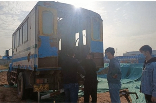
The procedure was executed using an LT-20A static probing engineering vehicle, which employed a helical ground anchor for counterforce and featured an automatic balance adjustment device. The investigation utilized double-bridge static probing equipment, developed domestically in China. The equipment’s probe had a tip cross-sectional area of 15 , while the side friction sleeve covered an area of 600 . Data collection was conducted through an LMC-310 automatic data acquisition system, complemented by a data processing microcomputer system. The probe advanced at a rate of 2 cm/s, recording data at every 10 cm of penetration, thereby ensuring continuous measurements of and . The specifications of the probe is shown in Table 1.

Table 1.

The specifications of the probe.

Probe types	Cone base		Cone tip	Friction sleeve
	Cross-sectional area ()	Diameter (mm)	Angle (°)	Length (cm)	Surface area (cm2 )	Effective area ratio
CPT probe	10	35.7	60	13.37	150	–

Sampling sites

CPT experiments at five sites in the Kaifeng area were executed in this study, incorporating geological and geotechnical investigation reports along with laboratory soil test data. The CPT field tests are shown in Fig. 1. These sites are part of the Yellow River alluvial plain, characterized by a relatively flat topography. Data from the first four sites were utilized for training and testing the model, while data from site 5 were used to validate the model.

Figure 1.

CPT field test image.

Dataset

Physical indicators of site soils

Frequent historical floods of the Yellow River have led to the formation of sediment layers along its banks. The investigation methods employed included drilling for samples, conducting geotechnical laboratory tests, CPT, and standard penetration tests. The groundwater level at the test site ranged from 0.8 to 10.1 meters, with the depth of the cone penetration tests extending from 10 to 35 meters. Drilling for samples and geotechnical laboratory tests were conducted near each CPT borehole to ascertain the groundwater level. By comparing and validating the data from CPT tests, drilling, and laboratory experiments, the relationship between CPT test data and soil types was explored. Based on the data from CPT tests, drilling, and laboratory experiments, the survey area, approximately 80 meters thick, predominantly contains four types of soils: silty clay, silt, fine sand, and medium sand, each exhibiting distinct physical and mechanical properties as outlined in Table 2. The study in this paper is based on the range of variation in physical indicators of this soil type. For soils exhibiting physical property indicators significantly beyond this range, validation against actual test data is recommended.

Table 2.

The physical and mechanical property indicators of each soil type.

No.	Soil type	Water content (%)	Density (g/cm3)	Porosity	Liquid limit (%)	Plastic limit (%)	Internal friction angle (°)
1	Silty clay	23.6–32.9	1.78–1.95	0.760–0.977	28.9–38.2	16.7–24.8	17–20
2	Silt	22.6–29.6	1.68–2.00	0.656–0.972	25.6–38.2	16.7–22.4	23–25
3	Fine sand	23.1–25.6	1.82–1.98	0.730–0.983	–	–	24–28
4	Medium sand	21.3–24.2	1.81–2.00	0.721–0.984	–	–	30–34

Test result

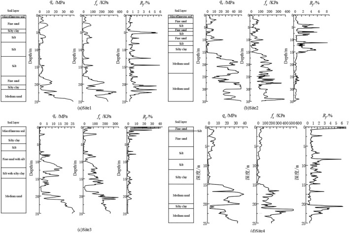
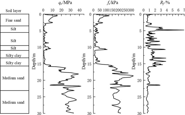
Figure 2 illustrates the typical CPT test hole profiles and soil layer distributions at the experimental sites. Sequentially, the diagrams depict drilling soil layers, , and , The formula for is as follows:

1

In Kaifeng area, the predominant soil layers consist of silty clay, silt, fine sand, and medium sand. The analysis of graphical data demonstrates significant fluctuations in , and with depth. Notably, fs is significantly greater than , yet their trends of variation are nearly identical. Silty clay layers are characterized by lower and higher values, in contrast to medium sand layers, which exhibit an inverse relationship with higher and lower . Furthermore, the graphs highlight considerable variability in these parameters across mixed silty clay and medium sand layers.

Figure 2.

Typical CPT test borehole profile at test sites.

Data analysis

Analysis of soil sampling data from four locations within the CPT detection depth range reveals four soil types: silty clay, silt, fine sand, and medium sand. The surface layers at these sites, predominantly composed of disturbed soil, exhibiting complex physical and mechanical properties that do not accurately represent the intrinsic characteristics of the underlying soil strata. Consequently, mixed layers containing various soil types fail to provide a precise representation of individual soil properties. To objectively evaluate the efficacy of different soil classification methods, CPT test data from surface and mixed layers were omitted from analysis.

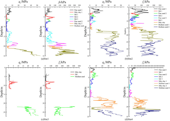
In this research, eight representative CPT test holes from the sites were selected for analysis, examining the correlation between qc and fs with depth across various soil strata. Figure 3 illustrates distinct correlations between CPT test parameters and depth. At Site 1, qc exhibits a negative correlation with depth in the silt layer and a positive correlation in the medium sand layer, whereas fs correlates positively with depth in the silty clay layer. At Site 2, both qc and fs display a negative correlation with depth in the fine sand layer and a positive correlation in the silty clay layer. Site 3’s qc shows a positive correlation with depth in the medium sand layer, with fs negatively correlated in the silty clay layer. For Site 4, qc correlates positively with depth in the medium sand layers and negatively in the silt layer, while fs correlates positively with depth in the silty clay layer and negatively in the fine sand and medium sand layers.

Figure 3.

The curves depicting the variations of CPT test parameters with depth(The solid line and dashed line represent one CPT test hole each).

Validation set data

To further validate the trained model’s applicability in the local area, data were gathered from Site 5. The physical and mechanical property indicators of various soil types at Site 5 correspond to those of the four previously mentioned experimental sites. Figure 4 illustrates the typical CPT test profile and soil layer distribution in the boreholes.

Figure 4.

Typical CPT test borehole profile at validation site.

Data pre-processing

The CPT generates a substantial volume of data, which may include anomalies not pertinent to the overall study’s scope.Thus, prior to analysis, it is imperative to filter out these anomalies to ensure data reliability³. Current methodologies for outlier detection encompass the Dixon, Chauvenet’s, t-test, Monte Carlo, Grubbs’, scatter plot, and the three standard deviations () methods.In this study, 133 test holes were drilled across five experimental sites, yielding extensive data. The method, applied in both positive and negative directions, was prioritized for preliminary data screening to expedite the process.

The method dictates the exclusion of data points when the absolute difference between a sample and the mean exceeds three times the standard deviation.

2

where , is the standard deviation.

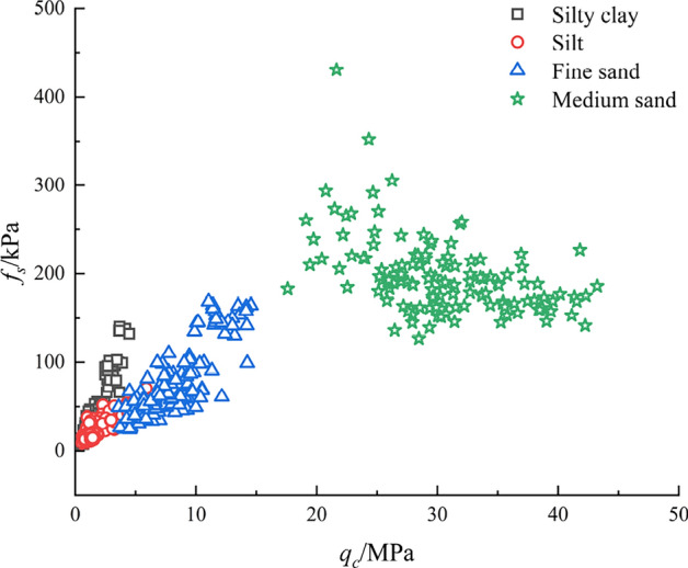
Following the method, the processed CPT test data were reassessed. Table 3 details the distribution of processed test holes and soil sample counts by type. Figure 5 illustrates the distribution of these data.

Table 3.

The distribution of CPT test holes and the number of soil samples for each soil type.

Site	Number of CPT holes	Silty clay	Silt	Fine sand	Medium sand
1	27	49	79	52	22
2	26	26	77	74	36
3	20	20	20	0	20
4	28	49	48	24	53
5	32	46	65	53	44
Total	133	190	289	203	175

Figure 5.

Data distribution.

Pearson’s correlation coefficient

The correlation coefficient (CC) measures the strength of the linear relationship between independent and dependent variables. Several methods can be used to determine correlation, including linear or curvilinear correlation, the scatter diagram method, Pearson’s product-moment correlation coefficient, and Spearman’s rank correlation coefficient. The classification of relationships based on the range of correlation coefficients is presented in Table 4²³.

Table 4.

Relationship level.

Correlation coefficient	Relationship level
–	Very strong
–	Strong
–	Moderate
–	Weak
–	No relationship

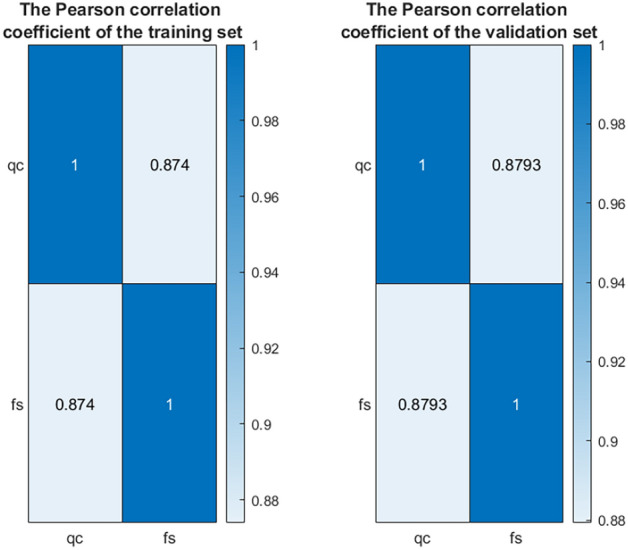
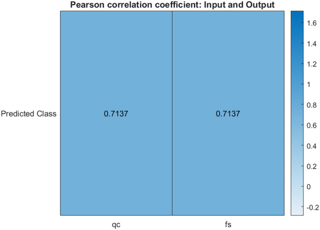
The Pearson correlation coefficients between the variables qc and fs in the two datasets are shown in Fig. 6. In both datasets, the correlation between and is notably high (close to 1), indicating a strong linear relationship between these two variables. Figure 7 presents the Pearson correlation coefficients between the input variables ( and ) and the model’s predicted classes. The correlation remains strong (approximately 0.7137), suggesting that not only is there a strong relationship between the input variables themselves, but also a significant correlation between these inputs and the model’s outputs.

Figure 6.

Pearson correlation coefficient:input.

Figure 7.

Pearson correlation coefficient: input and output.

Sensitivity analysis

The cosine amplitude method is used to determine the sensitivity of the input parameters and . The following equation illustrates the cosine amplitude method^24–27:

3

where, represents sensitivity of the input variable ; represents value of the input variable at the k-th experiment;represents output value at the k-th experiment;N represents total number of experiments.

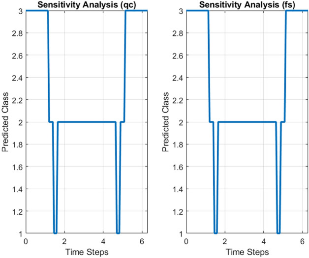
Figure 8 illustrates the time steps on the x-axis, which are 100 evenly spaced points ranging from 0 to 2, used to simulate the temporal variation of the input variables ( and ). The y-axis represents the predicted classes output by the SVM classifier. It can be observed that the predicted class changes at certain time steps when either qc or fs varies, indicating the model’s sensitivity to these input variables. The two subplots show similar patterns, reflecting the comparable impact of both input variables ( and ) on the model’s predictions. Since qc and fs both vary with the same amplitude and frequency, the similarity in their effects on the model results in similar patterns across the two plots.

Figure 8.

Sensitivity analysis.

Model

Previous studies have shown that the SVM with a linear kernel function, based on Kaifeng CPT data, outperformed other classifiers in soil layer classification but did not meet the accuracy standards required by engineering specifications. To address this issue, we considered using optimization algorithms. A comparative analysis of 25 commonly used algorithms was conducted to evaluate their respective optimization effects.

SVM

SVM, from a classification perspective, is a linear classifier designed to maximize the margin within the feature space. Its core principle involves identifying a hyperplane that maximizes the margin between two classes of sample data, thereby enhancing the model’s generalization capacity. Originally developed for binary classification, SVM uses a kernel function to map linearly inseparable samples from a low-dimensional space to a higher-dimensional one, converting linear inseparability into linear separability²⁸. The aim is to find the optimal hyperplane that minimizes classification errors^29,30. Samples within the maximized margin, known as “support vectors,” constitute the SVM model’s optimal solution.

Algorithm

The 25 selected algorithms are categorized into three main groups³¹. The first group consists of evolutionary algorithms, which are inspired by Darwin’s theory of natural selection, where the fittest individuals are selected and reproduced based on their fitness value. These algorithms include Genetic Algorithm (GA)³², Differential Evolution (DE)³³, Genetic Programming (GP)³⁴, and Biogeography-Based Optimizer (BBO)³⁵. The second group involves physics-based algorithms, which leverage concepts such as gravity, electromagnetic force, and equilibrium to develop metaheuristic approaches. Examples from this category include Simulated Annealing (SA)³⁶, Gravitational Search Algorithm (GSA)³⁷, Optics-Inspired Optimization (OIO)³⁸, Thermal Exchange Optimization (TEO)³⁹, Atom Search Optimization (ASO)⁴⁰, and Quantum-Based Avian Navigation Optimizer Algorithm (QANA)⁴¹. Lastly, the study explored swarm intelligence (SI) algorithms, which model the collective behavior of animals or insects working together and interacting with their environment. Algorithms in this group include Ant Colony Optimization (ACO)⁴², Particle Swarm Optimization (PSO)⁴³, Artificial Bee Colony (ABC)⁴⁴, Cuckoo Optimization Algorithm (COA)⁴⁵, Krill Herd (KH)⁴⁶, Bat Algorithm (BA)⁴⁷, Firefly Optimization Algorithm (FFA)⁴⁸, Grey Wolf Optimization (GWO)⁴⁹, Crow Search Algorithm (CSA)⁵⁰, Whale Optimization Algorithm (WOA)⁵¹, Sailfish Optimizer (SFO)⁵², Horse Herd Optimization Algorithm (HOA)⁵³, Starling Murmuration Optimizer (SMO)⁵⁴, Gorilla Troops Optimizer (GTO)⁵⁵ and Mountain Gazelle Optimizer (MGO)⁵⁶.Each of the aforementioned algorithms has its own advantages and is supported by well-established theoretical foundations. They have already been widely applied across various fields.

The optimization algorithm can be used to optimize the hyperparameters of the Support Vector Machine (SVM). SVM has several hyperparameters that need to be tuned, including the kernel function type (Kernel Function), kernel scale (Kernel Scale), penalty factor (Box Constraint), and the degree of the polynomial kernel (Polynomial Order).The initial parameters required by different algorithms vary, making manual tuning both time-consuming and difficult to standardize across algorithms. To address this, grid search-a hyperparameter optimization technique that systematically explores predefined parameter combinations using exhaustive search-was introduced before each algorithm⁵⁷. By utilizing grid search to find the optimal parameter settings, the process across algorithms becomes more consistent, thereby improving the comparability of results.

Monte Carlo simulation

Monte Carlo simulation is a statistical method that employs random sampling to perform numerical computations, simulating system behavior to estimate its overall performance. It is particularly effective for solving high-dimensional problems that cannot be addressed analytically. The advantages of Monte Carlo simulation include its broad applicability and flexibility, making it capable of handling complex, multidimensional problems. Additionally, the method easily accommodates various distributions and stochastic processes, offering high scalability⁵⁸. Performing Monte Carlo simulations on the training dataset helps enhance the model’s robustness and generalization ability. When cross-validated with the validation set, it provides a more comprehensive and objective assessment of the model’s performance.

Evaluation indicators

The analysis of the ML model results includes the confusion matrix, receiver operating characteristic (ROC) curve, and ten key performance metrics: overall accuracy (OA), precision (P), recall (R), score, Matthews correlation coefficient (MCC), average class accuracy (ACA), false omission rate (FOR), false discovery rate (FDR), false negative rate (FNR), and false positive rate (FPR).The six metrics—OA, P, R, score, MCC, and ACA—are considered better when higher, while the four metrics—FOR, FDR, FNR, and FPR—are preferred to be lower^11,59.

Considering that the focus of this study is multi-class classification and varying sample sizes, the average metrics for each model are calculated using weighted coefficients based on the proportions of samples from silty clay, silt, fine sand, and medium sand. For example, the calculation formulas for average precision (AP) and average recall (AR) are as follows:

4

5

where, , , , and correspond to the precision for silty clay, silt, fine sand, and medium sand samples, respectively; , , , and to the recall for each soil type; , , , and to the sample proportions of each soil type, respectively.

Result

This section focuses on the model’s stability and the evaluation of the trained model’s performance on the validation dataset. The assessment covers various aspects, including key performance metrics, the confusion matrix, and the ROC curve, providing detailed insights into the model’s effectiveness and optimization.

Monte Carlo simulation

This section presents three significant results obtained through Monte Carlo simulation, including the SVM model without algorithm optimization, the model optimized with OIO, and the model optimized with TEO.This section presents three significant results obtained from the Monte Carlo simulation are shown in Fig. 9: the SVM model without algorithm optimization, the model optimized with OIO, and the model optimized with TEO. The results show that the optimized models exhibit a tighter data distribution, improved classification stability, and higher accuracy within the concentrated distribution range compared to the unoptimized SVM model. Notably, the upper bound of accuracy for the optimized models follows the order: TEO> OIO > SVM.

Figure 9.

Accuracy distribution of the Monte Carlo simulation.

Key performance metrics

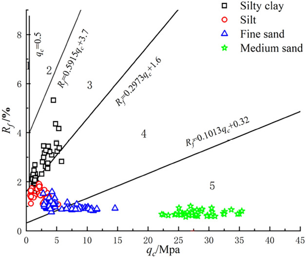
To evaluate the effectiveness of the model, we compared it with the traditional soil classification standard, the ’Code for in-situ measurement of railway engineering geology,’⁶⁰ which utilizes and for classification, using data from the validation set (Site 5). Figure 10 illustrates the distribution of CPT test data according to the ’code’ classification standard,with Table 5 detailing the classification accuracy.

Figure 10.

The soil classification results based on ’code’ soil classification chart.

Table 5.

The distribution of CPT test holes and the number of soil samples for each soil type.

Engineering classification of soils	The soil classification zones in the diagram	Accuracy
Silty clay	Zone 3	0.717
Silt	Zone 4	1.0
Fine sand	Zone 5	0.528
Medium sand	Zone 5	1.0
Overall(mean value)	from Zone 3 to 5	0.817

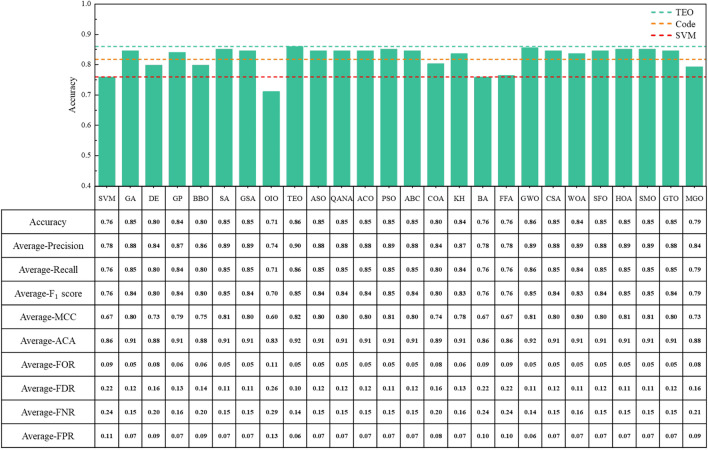
Based on Fig. 10 and Table 5, it can be observed that the ’Code for in-situ measurement of railway engineering geology’ achieved an overall classification accuracy of 0.817 for this experimental dataset.Overall accuracy refers to the proportion of correctly classified data points relative to the total number of data points.The classification of silt and medium sand was accurate, but there were significant misclassifications for silty clay and fine sand. Figure 11 shows four key performance metrics for the original SVM model and the models optimized by various algorithms. Among the 25 algorithms, 23 improved the classification accuracy of SVM, with 18 achieving an accuracy higher than that specified by the ’Code,’ indicating potential value for practical application. Notably, the SVM model optimized by TEO achieved a classification accuracy of 0.86, which represents a 10% improvement over the original SVM model (0.76) and a 4.3% improvement over the ’Code’ (0.817). Furthermore, the model optimized using TEO achieved the highest values across six performance metrics: OA, P, R, score, MCC, and ACA. Among these, OA, P, and MCC are the only metrics with the maximum values. Similarly, FOR, FDR, FNR, and FPR reached their minimum values, with FDR being the only metric showing the lowest value.

Figure 11.

Key performance metrics of the SVM after algorithm optimization.

Interestingly, it is also noteworthy that while the OIO-optimized model outperforms the initial SVM model in terms of accuracy during the Monte Carlo simulation, it performs the worst across all 10 evaluation metrics and shows poor performance on a completely new validation dataset. This suggests that the applicability of the OIO model is limited. In contrast, the TEO-optimized model demonstrates significantly better adaptability, maintaining stable performance on the validation set.

Confusion matrix

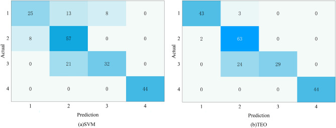
Figure 12 only presents the confusion matrices for the unoptimized SVM model and the TEO-optimized model on the validation set. The changes observed with other optimization algorithms follow a similar pattern to those of TEO.These matrices illustrate model performance, with rows representing predicted values and columns representing actual values. Correct classifications are displayed in the diagonal elements, while misclassifications appear in the off-diagonal elements. In the matrices, ‘1’ represents silty clay, ‘2’ represents silt, ‘3’ represents fine sand, and ‘4’ represents medium sand.

Figure 12.

The confusion matrix of the validation set.

Analysis of the confusion matrices in Fig. 12 reveals that the optimized model significantly improved the accuracy in identifying silty clay, with a marked reduction in misclassifications of silty clay as silt or fine sand. The accuracy in identifying silt also increased. Furthermore, the optimized model achieved nearly 100% accuracy in recognizing medium sand, which can be attributed to the distinct differences in and values between medium sand and other soil types, resulting in minimal overlap with other categories. However, both before and after optimization, the models tended to misclassify nearly half of the fine sand samples as silt, regardless of the kernel function used. The overlapping data points among silty clay, silt, and fine sand present a challenge for SVM models in achieving accurate classification.

ROC curve

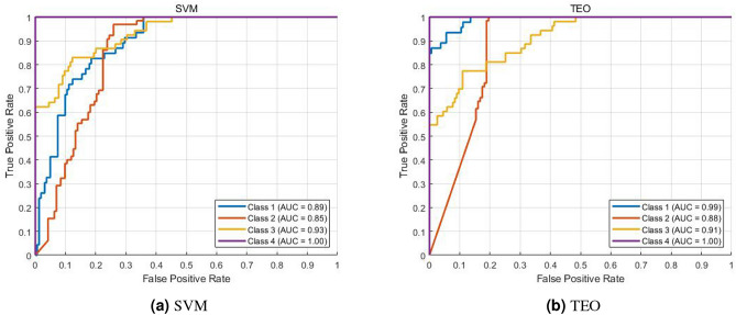
The ROC curve was a critical statistical method, which evaluates the quality of classification and detection by plotting the false positive rate (FPR) against the true positive rate (TPR). Model performance is assessed by the AUC,measuring classification quality. The two most important formulas for it are as follows:

6

7

AUC, ranging from 0 to 1, reflects classification accuracy: values closer to 1 indicate better performance. Specifically, AUC values>0.5 suggest acceptable accuracy, with values between 0.5 and 0.7 indicating low accuracy and those from 0.7 to 0.9 denoting moderate accuracy. The model under consideration has an AUC of 0.89, indicating moderate accuracy.

Based on the analysis of Fig. 13a,b, it is evident that the AUC of silty clay significantly increased after algorithm optimization, while silt showed a moderate increase, and fine sand experienced a slight decrease. Medium sand consistently achieved high AUC, indicating 100% classification accuracy for medium sand. These patterns and characteristics are consistent with the confusion matrix results.

Figure 13.

The ROC curve.

In conclusion, most algorithms contributed to improving the classification accuracy of SVM for soil types, outperforming the traditional engineering standard, ’Code for in-situ measurement of railway engineering geology.’ These models not only help reduce the classification workload and enhance efficiency but also provide superior results, making them a practical alternative to traditional classification methods and demonstrating their suitability for engineering applications.

Conclusions

This study utilized a SVM model based on CPT data, which was optimized using 25 different algorithms. The model was validated through Monte Carlo simulations and independent site data, followed by a comprehensive evaluation using confusion matrices, ROC curves, and ten key performance indicators. The results indicate that 23 of the algorithms improved the classification performance of the SVM model, with 18 algorithms achieving classification accuracies exceeding the standards outlined in the “Specification for In-situ Testing of Railway Engineering Geology.” This achievement not only highlights the low-interference advantage of CPT technology but also introduces a novel soil classification method through machine learning, independent of traditional empirical knowledge. The SVM model trained with CPT data has been experimentally validated for effective soil classification in specific regions, offering new perspectives for the field.

Due to the minimal particle size variation in fine-grained soils, the associated resistance values are very similar, resulting in blurred boundaries between soil types. This presents a challenge in accurately distinguishing between clay and silt.

The optimized model has now surpassed industry standards in classification accuracy and is capable of effectively minimizing subjective errors caused by varying levels of expertise among operators. This advancement provides valuable objective support for engineering decisions and soil management practices under complex site conditions.

Furthermore, to assess the model’s generalizability in different geological contexts, future work should focus on collecting a broader range of high-quality test data and developing more precise models to enhance the automation and accuracy of soil classification. Adapting algorithms to different soil conditions will be a crucial area of future research.

Author contributions

H.B., Z.S., J.B., and J.Z. conceptualized the study. H.B., Z.S., J.B., and X.X. developed the methodology. Z.S., J.B., and Z.Q. contributed to data curation. Z.S., and J.B. Wrote the original draft of the report and authored the code. Z.S.,J.B.,and Z.Q. were involved in the investigation, formal analysis, validation, and visualization. H.B., J.Z. and X.X. contributed to review and editing of the report. H.B., Z.Q., J.Z. and X.X. contributed to supervision of the study. H.B. and J.Z. were responsible for funding, resources and project administration. H.B., Z.S., J.Z., and X.X. had final responsibility for the decision to submit for publication. All authors had access to all data. H.B.,J.B. and Z.Q. verifed the data. All authors reviewed the manuscript.

Data availability

The data that support the findings of this study are available from the corresponding author upon reasonable request.

Declarations

Competing interests

The author(s) declare no competing interests.

References

- 1.L., S. & W., Y. On the current situation and development of static penetration technology (cpt) in china. Chin. J. Geotech. Eng. 553–556. http://www.cgejournal.com/article/id/11468 (2004).
- 2.Robertson, & K, P. Interpretation of cone penetration tests: A unified approach. Can. Geotech. J.46, 1337–1355. 10.1139/T09-065 (2009). [Google Scholar]
- 3.Z., M. Kaifeng city and the yellow river. J. Beijing Union Univ. 133–138, 10.16255/j.cnki.ldxbz.2002.01.033 (2002).
- 4.Khatti, J. & Grover, K. S. Assessment of hydraulic conductivity of compacted clayey soil using artificial neural network: An investigation on structural and database multicollinearity. Earth Sci. Inform.[SPACE]10.1007/s12145-024-01336-0 (2024). [Google Scholar]
- 5.Khatti, J. & Grover, K. S. Determination of suitable hyperparameters of artificial neural network for the best prediction of geotechnical properties of soil. Int. J. Res. Appl. Sci. Eng. Technol.10, 4934–4961 (2022). [Google Scholar]
- 6.Khatti, J. & Grover, K. S. Assessment of the uniaxial compressive strength of intact rocks: An extended comparison between machine and advanced machine learning models. Multisc. Multidiscip. Model. Exp. Des.[SPACE]10.1007/s41939-024-00408-4 (2024). [Google Scholar]
- 7.Khatti, J. & Grover, K. S. Assessment of uniaxial strength of rocks: A critical comparison between evolutionary and swarm optimized relevance vector machine models. Transp. Infrastruct. Geotechnol.[SPACE]10.1007/s40515-024-00433-3 (2024). [Google Scholar]
- 8.Khatti, J. & Grover, K. S. Estimation of intact rock uniaxial compressive strength using advanced machine learning. Transp. Infrastruct. Geotechnol.11, 1989–2022. 10.1007/s40515-023-00357-4 (2024). [Google Scholar]
- 9.Khatti, J. & Grover, K. S. Prediction of uniaxial strength of rocks using relevance vector machine improved with dual kernels and metaheuristic algorithms. Rock Mech. Rock Eng.[SPACE]10.1007/s00603-024-03849-y (2024). [DOI] [PMC free article] [PubMed] [Google Scholar]
- 10.Kumar, M., Kumar, D. R., Khatti, J., Samui, P. & Grover, K. S. Prediction of bearing capacity of pile foundation using deep learning approaches. Front. Struct. Civil Eng.[SPACE]10.1007/s11709-024-1085-z (2024). [Google Scholar]
- 11.Khatti, J. et al. Cone penetration test-based assessment of liquefaction potential using machine and hybrid learning approaches. Multisc. Multidiscip. Model. Exp. Des.[SPACE]10.1007/s41939-024-00447-x (2024). [Google Scholar]
- 12.Hossein, R. M. & Hojjat, A. Novel machine-learning model for estimating construction costs considering economic variables and indexes. J. Constr. Eng. Manag.144, 04018106. 10.1061/(ASCE)CO.1943-7862.0001570 (2018). [Google Scholar]
- 13.C, P. & TA, M. Dams, dam costs and damnable cost overruns. J. Hydrol. X3, 100026. 10.1016/j.Hydra.2019.100026 (2019). [Google Scholar]
- 14.Arsalan, M., Reza, N. H. & Mokhtar, M. Optimized machine learning modelling for predicting the construction cost and duration of tunnelling projects. Autom. Constr.139, 104305. 10.1016/j.autcon.2022.104305 (2022). [Google Scholar]
- 15.U, K. P. & P, G. E. Prediction of soil composition from cpt data using general regression neural network. J. Comput. Civ. Eng.20, 281–289. 10.1061/(ASCE)0887-3801(2006)20:4(281) (2006). [Google Scholar]
- 16.Guojun, C., Songyu, L. & J, P. A. Identification of soil strata based on general regression neural network model from cptu data. Mar. Georesour. Geotechnol.33, 229–238. 10.1080/1064119X.2013.843046 (2015). [Google Scholar]
- 17.Cormac, R., Kenneth, G., Lovorka, L. & Danijela, J.-K. Automatic classification of fine-grained soils using cpt measurements and artificial neural networks. Adv. Eng. Inform.36, 207–215. 10.1016/j.aei.2018.04.003 (2018). [Google Scholar]
- 18.Kumar, D. S. & Kumar, B. P. Utilization of self-organizing map and fuzzy clustering for site characterization using piezocone data. Comput. Geotech.36, 241–248. 10.1016/j.compgeo.2008.02.005 (2009). [Google Scholar]
- 19.H, E. G., Simon, O., Anna, F. & Marte, R. Learning decision boundaries for cone penetration test classification. Comput.-Aid. Civil Infrastruct. Eng.36, 489–503. 10.1111/mice.12662 (2021). [Google Scholar]
- 20.Stefan, R. & Franz, T. Cpt data interpretation employing different machine learning techniques. Geosciences11, 265. 10.3390/geosciences11070265 (2021). [Google Scholar]
- 21.Zi-Jun, C., Shuo, Z., Dian-Qing, L. & Kok-Kwang, P. Bayesian identification of soil stratigraphy based on soil behaviour type index. Can. Geotech. J.56, 570–586. 10.1139/cgj-2017-0714 (2019). [Google Scholar]
- 22.Hui, W., Xiangrong, W. & Florian, W. J. A bayesian unsupervised learning approach for identifying soil stratification using cone penetration data. Can. Geotech. J.56, 1184–1205. 10.1139/cgj-2017-0709 (2019). [Google Scholar]
- 23.Khatti, J. & Grover, K. A study of relationship among correlation coefficient, performance, and overfitting using regression analysis. Int. J. Sci. Eng. Res13, 1074–1085 (2022). [Google Scholar]
- 24.Samadi, H., Hassanpour, J., Rostami, J. & Khatti, J. Application of supervised learning algorithms to predict engineering characteristics of soft to strong rock masses using actual tbm performance data. in ARMA US Rock Mechanics/Geomechanics Symposium, D022S023R001. 10.56952/ARMA-2024-0036 (ARMA, 2024).
- 25.Khatti, J. & Polat, B. Y. Assessment of short and long-term pozzolanic activity of natural pozzolans using machine learning approaches. In Structures68, 107159. 10.1016/j.istruc.2024.107159 (2024) ((Elsevier)). [Google Scholar]
- 26.Hosseini, S. et al. Assessment of the ground vibration during blasting in mining projects using different computational approaches. Sci. Rep.13, 18582. 10.1038/s41598-023-46064-5 (2023). [DOI] [PMC free article] [PubMed] [Google Scholar]
- 27.Fissha, Y. et al. Predicting ground vibration during rock blasting using relevance vector machine improved with dual kernels and metaheuristic algorithms. Sci. Rep.14, 20026. 10.1038/s41598-024-70939-w (2024). [DOI] [PMC free article] [PubMed] [Google Scholar]
- 28.Z, L. et al. Research on estimating atmospheric optical turbulence profiles based on support vector machine. Acta Optica Sinica42, 43–51. 10.3788/aos202242.0101001 (2022). [Google Scholar]
- 29.Z, W. Research on Text Classification Algorithms Based on Support Vector Machine and Neural Networks. Master’s thesis, Nanjing: Nanjing University of Posts and Telecommunications. 10.27251/d.cnki.gnjdc.2019.000523 (2019).
- 30.L, Y. Research on Vehicle Type Classification Technology Based on CNN, CRNN, and SVM for Audio Signals. Master’s thesis, Chongqing: Chongqing University of Technology. 10.27753/d.cnki.gcqgx.2022.000732 (2022).
- 31.Hasmat, M. et al.Metaheuristic and Evolutionary Computation: algorithms and applications, vol. 916 (Springer, 2021). https://link.springer.com/book/10.1007/978-981-15-7571-6.
- 32.H, H. J. Genetic algorithms. Sci. Am.267, 66–73 (1992). Available at: https://www.jstor.org/stable/24939139.
- 33.Rainer, S. & Kenneth, P. Differential evolution-a simple and efficient heuristic for global optimization over continuous spaces. J. Glob. Optim.11, 341–359 (1997). [Google Scholar]
- 34.R, K. J. Genetic Programming II: Automatic Discovery of Reusable Programs (MIT Press, 1994). https://dl.acm.org/doi/abs/10.5555/183460.
- 35.Dan, S. Biogeography-based optimization. IEEE Trans. Evol. Comput.12, 702–713. 10.1109/TEVC.2008.919004 (2008). [Google Scholar]
- 36.Dimitris, B. & John, T. Simulated annealing. Stat. Sci.8, 10–15. 10.1214/ss/1177011077 (1993). [Google Scholar]
- 37.Esmat, R., Hossein, N.-P. & Saeid, S. Gsa: A gravitational search algorithm. Inf. Sci.179, 2232–2248. 10.1016/j.ins.2009.03.004 (2009). [Google Scholar]
- 38.Husseinzadeh, K. A. A new metaheuristic for optimization: Optics inspired optimization (oio). Comput. Oper. Res.55, 99–125. 10.1016/j.cor.2014.10.011 (2015). [Google Scholar]
- 39.Ali, K. & Armin, D. A novel meta-heuristic optimization algorithm: Thermal exchange optimization. Adv. Eng. Softw.110, 69–84. 10.1016/j.advengsoft.2017.03.014 (2017). [Google Scholar]
- 40.Weiguo, Z., Liying, W. & Zhenxing, Z. Atom search optimization and its application to solve a hydrogeologic parameter estimation problem. Knowl.-Based Syst.163, 283–304. 10.1016/j.knosys.2018.08.030 (2019). [Google Scholar]
- 41.Hoda, Z., H, N.-S.M. & H, G. A. Qana: Quantum-based avian navigation optimizer algorithm. Eng. Appl. Artif. Intell.104, 104314. 10.1016/j.engappai.2021.104314 (2021). [Google Scholar]
- 42.Marco, D., Mauro, B. & Thomas, S. Ant colony optimization. IEEE Comput. Intell. Mag.1, 28–39. 10.1109/MCI.2006.329691 (2006). [Google Scholar]
- 43.James, K. & Russell, E. Particle swarm optimization. in Proceedings of ICNN’95-international conference on neural networks, vol. 4, 1942–1948 (IEEE). 10.1109/ICNN.1995.488968 (1995).
- 44.Dervis, K. et al. An idea based on honey bee swarm for numerical optimization. Tech. Rep., Technical report-tr06, Erciyes university, engineering faculty, computer. https://abc.erciyes.edu.tr/pub/tr06_2005.pdf (2005).
- 45.Ramin, R. Cuckoo optimization algorithm. Appl. Soft Comput.11, 5508–5518. 10.1016/j.asoc.2011.05.008 (2011). [Google Scholar]
- 46.Hossein, G. A. & Hossein, A. A. Krill herd: a new bio-inspired optimization algorithm. Commun. Nonlinear Sci. Numer. Simul.17, 4831–4845. 10.1016/j.cnsns.2012.05.010 (2012). [Google Scholar]
- 47.Xin-She, Y. & Amir, H. G. Bat algorithm: A novel approach for global engineering optimization. Eng. Comput.29, 464–483. 10.1108/02644401211235834 (2012). [Google Scholar]
- 48.Iztok, F., Iztok, F. J., Xin-She, Y. & Janez, B. A comprehensive review of firefly algorithms. Swarm Evol. Comput.13, 34–46. 10.1016/j.swevo.2013.06.001 (2013). [Google Scholar]
- 49.Seyedali, M., Mohammad, M. S. & Andrew, L. Grey wolf optimizer. Adv. Eng. Softw.69, 46–61. 10.1016/j.advengsoft.2013.12.007 (2014). [Google Scholar]
- 50.Alireza, A. A novel metaheuristic method for solving constrained engineering optimization problems: Crow search algorithm. Comput. Struct.169, 1–12. 10.1016/j.compstruc.2016.03.001 (2016). [Google Scholar]
- 51.Seyedali, M. & Andrew, L. The whale optimization algorithm. Adv. Eng. Softw.95, 51–67. 10.1016/j.advengsoft.2016.01.008 (2016). [Google Scholar]
- 52.Soodeh, S., Reza, N. H. & Khatibi, B. V. The sailfish optimizer: A novel nature-inspired metaheuristic algorithm for solving constrained engineering optimization problems. Eng. Appl. Artif. Intell.80, 20–34. 10.1016/j.engappai.2019.01.001 (2019). [Google Scholar]
- 53.Farid, M., Gholamreza, A. & Mohsen, R. Horse herd optimization algorithm: A nature-inspired algorithm for high-dimensional optimization problems. Knowl.-Based Syst.213, 106711. 10.1016/j.knosys.2020.106711 (2021). [Google Scholar]
- 54.Hoda, Z. & H, N.-S.M. Starling murmuration optimizer: A novel bio-inspired algorithm for global and engineering optimization. Comput. Methods Appl. Mech. Eng.392, 114616. 10.1016/j.cma.2022.114616 (2022). [Google Scholar]
- 55.Benyamin, A., Farhad, S. G. & Seyedali, M. Artificial gorilla troops optimizer: A new nature-inspired metaheuristic algorithm for global optimization problems. Int. J. Intell. Syst.36, 5887–5958. 10.1002/int.22535 (2021). [Google Scholar]
- 56.Benyamin, A., Soleimanian, G. F., Nima, K. & Seyedali, M. Mountain gazelle optimizer: A new nature-inspired metaheuristic algorithm for global optimization problems. Adv. Eng. Softw.174, 103282. 10.1016/j.advengsoft.2022.103282 (2022). [Google Scholar]
- 57.Marc, C. & Bart, D. M. Hyperparameter search in machine learning. arXiv preprint arXiv:1502.0212710.48550/arXiv.1502.02127 (2015).
- 58.Aladejare, A. E., Idowu, K. A. & Ozoji, T. Reliability of Monte Carlo simulation approach for estimating uniaxial compressive strength of intact rock. Earth Sci. Inform.[SPACE]10.1007/s12145-024-01262-1 (2024). [Google Scholar]
- 59.Ali, D., Behzad, M. & Ghassem, H. Identification of dispersive soils via computational intelligence. Eur. J. Soil Sci.74, e13346. 10.1111/ejss.13346 (2023). [Google Scholar]
- 60.Code for in-situ measurement of railway engineering geology (2003).
Associated Data
This section collects any data citations, data availability statements, or supplementary materials included in this article.
Data Availability Statement