The development of an efficient artificial intelligence-based classification approach for colorectal cancer response to radiochemotherapy: deep learning vs. machine learning

Abstract

Colorectal cancer (CRC) is a form of cancer that impacts both the rectum and colon. Typically, it begins with a small abnormal growth known as a polyp, which can either be non-cancerous or cancerous. Therefore, early detection of colorectal cancer as the second deadliest cancer after lung cancer, can be highly beneficial. Moreover, the standard treatment for locally advanced colorectal cancer, which is widely accepted around the world, is chemoradiotherapy. Then, in this study, seven artificial intelligence models including decision tree, K-nearest neighbors, Adaboost, random forest, Gradient Boosting, multi-layer perceptron, and convolutional neural network were implemented to detect patients responder and non-responder to radiochemotherapy. For finding the potential predictors (genes), three feature selection strategies were employed including mutual information, F-classif, and Chi-Square. Based on feature selection models, four different scenarios were developed and five, ten, twenty and thirty features selected for designing a more accurate classification paradigm. The results of this study confirm that random forest, Gradient Boosting, decision tree, and K-nearest neighbors provided more accurate results in terms of accuracy, by 93.8%. Moreover, Among the feature selection methods, mutual information and F-classif showed the best results, while Chi-Square produced the worst results. Therefore, the suggested artificial intelligence models can be successfully applied as a robust approach for classification of colorectal cancer response to radiochemotherapy for medical studies.

Introduction

Colorectal cancer (CRC) is among the most prevalent cancer types and a leading cause of cancer-related deaths worldwide^1,2. CRC is the second and third most commonly diagnosed type of cancer among men and women, respectively³. In recent decades, the incidence of CRC has been increasing and development of it may be influenced by several parameters, including genetic and epigenetic factors, as well as environmental factors³. The occurrence of CRC is higher in developed countries compared to developing countries⁴. It is worth mentioning that colonoscopy and CT-colonoscopy are recommended diagnostic methods for patients with suspected CRC^5,6. Non-invasive diagnostic methods, including fecal occult blood tests, carcinoembryonic antigen (CEA) tests, and carbohydrate antigen tests, have limited sensitivity and specificity in detecting CRC and have not been associated with improved survival outcomes. Therefore, the main treatments for CRC include radiochemotherapy, surgery, and radiation therapy, which are often used in combination^7,8. Chemoradiotherapy is now considered a standard treatment for rectal cancer⁵. Furthermore, gene signatures that use microarray technology have shown that the gene expression patterns of tumor cells can distinguish between patients who respond well to chemoradiotherapy and those who are resistant to treatment⁶. The use of gene expression profiling, which involves biological examination and integrative computational biology, is commonly used to develop clinical classifiers for rectal cancer^9,10. This technique also helps predict patient response to treatment. One of the main obstacles in treating CRC is the development of resistance to treatment. However, molecular mechanisms and cancer biomarkers, such as DNA, RNA, protein, and metabolites, can help identify new targets for cancer research and improve tumor response, leading to more effective treatment methods that can overcome resistance⁶.

As mentioned earlier, in recent times, CRC has been characterized as a heterogeneous disease. It has been diagnosed as a major disease worldwide and globally, it is the second most common reason for cancer-related deaths. CRC is now recognized as a serious, highly prevalent cancer that is responsible for a large proportion of cancer mortalities worldwide¹¹.

One of the best solutions to improve CRC treatment is early diagnosis through analysis of biopsy images¹². Moreover, early CRC diagnosis enabled by artificial intelligence (AI) analysis of biopsy images can greatly improve patient outcomes^13,14. In recent years, there has been considerable attention on using AI in medicine^9,10,13,14. Researchers worldwide have utilized different AI approaches as an effective solution for predicting and classifying various cancers using available medical data^9,10,13,14. The classification of cancer with AI has received significant research attention, demonstrating AI’s potential for solving complex tasks^10,13,14. There are now many published studies validating the capabilities of AI for CRC classification, showing it is an active area of research with great promise¹⁵. Dimitriou et al. (2018)¹ addressed the issue of heterogeneity in CRC patients, where outcomes can vary despite similar staging. They studied a group of 173 patients using machine learning (ML) techniques and adhered to the current TNM guidelines. Xu et al. (2020)² used ML technology to analyze the risk of postoperative recurrence in patients with stage IV CRC. They evaluated four common ML algorithms, including logistic regression, decision tree, Gradient Boosting, and LightGBM, to make their predictions. The ML algorithms mentioned above can make individual predictions about the likelihood of a tumor coming back in individuals who have undergone surgery for stage IV CRC. Among these algorithms, Gradient Boosting and LightGBM were found to produce more accurate results. Moreover, the weight matrix generated by Gradient Boosting identified chemotherapy, age, LogCEA, CEA, and anesthesia time as factors associated with postoperative tumor recurrence. Wan et al. (2019)⁵ employed ML methods to detect signatures in circulating cell-free DNA (cfDNA) for early detection of cancer. Their study achieved high sensitivity and specificity in a significant cohort of early-stage colorectal cancer patients using machine learning techniques with cfDNA.

Bychkov et al. (2018)¹⁶ demonstrated the high precision of deep learning and ML in medical image analysis. Their study directly produced patient outcomes without the need for intermediate tissue classification. They evaluated digitized samples of tumor tissue microarrays from 420 CRC patients stained with haematoxylin–eosin and used integrated architectures to train a deep network for predicting CRC outcomes based on tumor tissue images. They suggest that deep learning methods can extract more predictive details of tissue morphology in CRC patients than an experienced human observer. Takamatsu et al. (2019)⁶ found that ML offered greater predictive capability than conventional methods. They developed a ML algorithm for predicting lymph node metastasis (LNM) in submucosal invasive (T1) CRC, which is important for determining treatment strategies after endoscopy. They also found that ML resulted in fewer false-negative cases than conventional methods. Whole slide images were identified as a potential option for selecting therapy procedures for T1 CRC. In their study, they compared the performance of current classification methods, such as deep learning, ML, and deep transfer learning, to determine the most effective approach. Also, Li et al. (2021)¹⁷ conducted an investigation and found that deep transfer learning was the most effective technique with an area under the curve of 0.7941 and accuracy of 0.7583. The study’s findings promote the use of effective methods in detecting LNM in CRC and simplifying appropriate treatment. The research suggests the use of ML techniques in cancer research for their high accuracy in early diagnosis and directing the selection of suitable therapy procedures. The study recommended using DNN based Relief attribute investigation algorithm and LightGBM based Relief attribute investigation to distinguish between non-cancerous and cancerous cells in colon cancer. In the application of ML models for classification of cancer cells, Nazari et al. (2021)¹⁸ evaluated several ML methods for classifying cancer cells, including Naive Bayes, logistic model trees (LMT), quadratic discriminant analysis (QDA), bagging, AdaBoost, and deep neural networks (DNN). They found that some of the suggested techniques were able to perform the classification with 100% precision. Based on these results, they concluded that ML methods like Naive Bayes that achieved perfect precision, can be a reliable approach for distinguishing between cancerous and non-cancerous cells. Moreover, Escorcia-Gutierrez et al. (2022)¹⁹ applied a novel galactic swarm optimization (GSO) with deep transfer learning model using the image-guided intervention (IGI) for CRC classification (GSODTL-C3M). The proposed GSODTL-C3M use the bilateral filtering (BF) algorithm for handling the presence of noise data. In addition to this, they have adopted the Adam optimizer with the mobile net algorithm for extracting the features. At the end of the modelling framework, the hybrid long short-term memory (LSTM) combined with the GSO algorithm was applied for CRC classification. According to the obtained results, and compared to the convolutional neural network (CNN) and the residual network (ResNet), it was found that, the GSODTL-C3M was more accurate and they exhibiting high classification performances taking into account the accuracy, recall, precision, F_score and the specificity calculated as the performances metrics. Gao et al. (2022)²⁰ used random forest (RF) classification algorithm for predicting the CRC using microbial relative abundance profiles (MRP). The most significant finding of the study was that the RF performances based on the MPR provided by centrifuge were higher than those estimated using MetaPhlAn2 and Bracken. Furthermore, it was found that, the RF classifier was more accurate compared to support vector machine (SVM) and least absolute shrinkage and selection operator (LASSO) classifiers. Li et al. (2023)²¹ compared between an ensemble of supervised ML models belonging into three categories namely: (i) deep learning, i.e., the CNN, (ii) the standalone multi-layer perceptron neural network (MLPNN), and (iii) three ensemble learning algorithm, i.e., the XGboost, LightGBM, and Catboost algorithms, for CRC classification using the combination of multi-scale whole slide images (WSI) and mass spectrometry imaging (MSI) data. They reported that, in one hand; CNN was less accurate compared to the other ML models and in the other hand, the LightGBM has better performances compared to the other models.

Xu et al. (2023)²² investigated the capability of new supervised deep learning model called attention-based multi-instance learning (MIL) for CRC classification using the formalin-fixed paraffin-embedded (FFPE) whole-slide images (WSI). Thus, several CNN were applied and compared for better classification of CRC having different architectures, i.e., 3-layer, 4-layer and 5-leyer CNN, and for extracting the features from images. From the obtained results, it was found that, 3-layer CNN was more accurate compared to the two others. In another study, Zhou et al. (2021)²³ used 1346 WSI collected from the data cancer genome atlas (TCGA) for classification purpose. They used the ResNet approach and results indicated superior classification accuracies with 94.6%. Lo et al. (2023)²⁴ compared between the subspace ensemble k-nearest neighbor (SEKNN), SVM, logistic regression (LR), and artificial neural network (ANN) for CRC using the feature ensemble vision transformer (FEViT). According to the obtained results, SEKNN was more accurate compared to SVM, ANN and LR, exhibiting an accuracy ranged from 79 to 94%, respectively. Schirris et al. (2022)²⁵ introduced a deep learning model called self-supervised pre-training and heterogeneity-aware deep multiple instance learning (DeepSMILE) for classification of tumor-annotated CRC dataset. Compared to the ImageNet pre-trained tile-supervised WSI-label learning (ImageNet), DeepSMILE was found to be more accurate exhibiting an overall classification accuracy nearly equal to 75%. Raghav et al. (2024)²⁶ examined the performances of several ML classifiers for classification of molecular subtypes of CRC using gene expression profiles. They compared between the MLPNN, AdaBoost, XGBoost, Bagging, Boosting, logistic regression (LR), decision trees (DT), KNN, and RF. The best classification accuracy of 79% was obtained using LR and AdaBoost, respectively. Chang et al. (2023)²⁷ developed a new hybrid model by combining the CNN and the self-attention model to predict microsatellite instability (MSI) of CRC. Compared to the Vision Transformers (ViT) deep learning, and EfficientNet, attention-based multiple instance learning (AttMIL), the proposed hybrid model was found to be more accurate exhibiting and overall accuracy of 95.4%.

Luo and Bocklitz (2023)²⁸ use the microsatellite instable or hypermutated (MSIMUT) and microsatellite stable (MSS) images for CRC classification. They compared between five deep learning models namely, DenseNet121, DenseNet201, InceptionV3, MobileNetV2, and ResNet50, SVM classifiers combined with the principal component analysis (PCA-SVM), and linear discriminant analysis (PCA-LDA). It was found that, the use of transfer learning concept helped in improving the classification accuracies. Kumar et al. (2023)²⁹ used the colorectal histology public dataset for developing a ML model on CRC classification. The authors proposed the CRC classification model based on convolutional neural network (CRCCN-Net) and they compared their performances with those of Xception, InceptionResNetV2, DenseNet121, VGG16 deep learning architectures. From the obtained results, it was found that the new proposed CRCCN-Net deep learning outperformed the other models exhibiting high classification accuracy of 93.50% compared to the values of 88.20%, 89.20%, 87.20%, and 90.40% obtained using the Xception, InceptionResNetV2, DenseNet121, and VGG16, respectively. In another study, and using the colon cancer gene expression dataset obtained from Kaggle, Arowolo et al. (2023)³⁰ compared between RF, KNN, and SVM classifiers for CRC classification, with and without principal component classification (PCA) dimensionality reduction tool. Without PCA, RF was found to be more accurate exhibiting an overall classification accuracy of 84% compared to the values of 77.75% and 81.00% obtained using SVM and KNN. Furthermore, with PCA, the classification performances of RF were found to be lawyers the best reaching a value of 96% compared to the values of 80.40% and 81.90% obtained using SVM and KNN, respectively. Parhami et al. (2023)³¹ compared between three deep learning models namely, CNN, LSTM and CNN + LSTM for the classification of CRC using a pre-processing clustered gene filtering (CGF) and indexed sparsity reduction (ISR) methods, using data from the cancer genome atlas (TCGA). Obtained results revealed that CNN was the most accurate model exhibiting an overall accuracy of 66.45% compared to the values of 40.89% and 41.20% obtained using LSTM and CNN + LSTM, respectively. Kim et al. (2021)³² compared between ResNet, DenseNet, and Inception V3 CNN models for CRC classification using the images obtained via colonoscopic biopsy. According to the obtained results it was demonstrated that the Res-net was more accurate compared to the DenseNet, and Inception V3 deep learning models with an accuracy of 94.9% compared to the values of 93.6% and 92.2%, respectively. Moreover, Su et al. (2022)³³ compared between SVM, RF and DT models for classification and diagnosis of CRC using gene expression profiling data from the cancer genome atlas (TCGA). RF had the best classification results with an accuracy of 99.81% compared to the values of 99.62% and 98.46% obtained using DT and SVM, respectively. Deep learning for single-cell RNAseq imputation has been used by Wang et al. (2023a)³⁴. In another study, Wang et al. (2024a)³⁵ use graph deep learning for modeling the spatial transcriptomics and domain detection. Wang et al. (2023b)³⁶ developed a new DFinder graph embedding-based approach for finding drug-food interactions. Wang et al. (2022)³⁷ use summary statistic imputation for improving findings of molecular QTL works based on considering small sample size data. The mendelian randomization was used by Wang et al. (2024b)³⁸ for identifying impacts of sarcopenia on risk and progression of Parkinson disease, and finally, Wang et al. (2024c)³⁹ developed a tool based on the web server approach for identifying the causality post the genome-wide association studies.

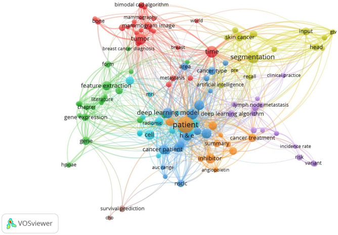
In this research, the application of decision tree (DT), K-nearest neighbors (KNN), AdaBoost, random forest (RF), Gradient Boosting (GB), multi-layer perceptron (MLP), and convolutional neural network (CNN) models was proposed for classifying CRC response to radiochemotherapy. Moreover, three reliable feature selection strategies have been applied including mutual information, F-classif, and Chi-Square for identifying the most relevant features in the dataset. As mentioned, this study is the first to propose multiple intelligent models, including decision tree, KNN, AdaBoost, RF, GB, MLPNN, and CNN, for robust classification of CRC response to radiochemotherapy. Also, based on the authors knowledge, this study is the first investigation of the mentioned paradigms for classification of CRC based on the GEO dataset. Figure 1 displays the primary keywords obtained from the literature review using the VOSviewer software (https://www.vosviewer.com/download)⁴⁰. It illustrates the utilization of various AI models for classification problems in medical cancer studies.

Fig. 1.

The literature review evaluation for conducting medical cancer research by various artificial intelligence approaches.

Methods

In this study, seven machine learning and deep learning models including DT, KNN, AdaBoost, RF, Gradient Boosting, MLP, and CNN were used for predicting CRC based on outputs of three feature selection strategies including MI, F-classif, and Chi-Square. Figure 2 illustrates the various steps involved in current research.

Fig. 2.

Workflow of the present study.

Decision tree

Decision tree (DT) as one of the classical ML is classified as non-parametric supervised learning models and it can be described as a structure resembling a tree, in which the leaves symbolize the labels assigned to outputs, and the branches indicate combinations of predictors that led to those particular results⁴¹. DT can be categorized into two types⁴² including classification and regression trees. Classification trees are applicable for discrete variables and regression trees are suitable for continuous variables. The process of modeling the decision tree typically involves two primary stages: (i) creating the trees, and (ii) refining the trees through pruning⁴¹. In most situations, pruning is necessary to remove unsuitable nodes from the tree. The pruning process can be handled using two categories of tree pruning, namely pre-pruning and post-pruning⁴¹. Moreover, in the concept of DT methodology, dataset’s impurity or randomness is evaluated using entropy⁴¹. Also, for checking segmentation information gain metric is applied. It is worth mentioning that the value of entropy ranges between 0 and 1.

There is an effective algorithm that characterized by initially generating a large-sized tree and then automatically removing unnecessary branches once it identifies the optimal pruning threshold. After tree pruning, the gain-ratio is calculated during the training stage as follows⁴¹:

1

where

2

3

where X and T are attribute and training dataset, respectively. More details about DT model can be found in⁴¹.

K-nearest neighbors

K-nearest neighbors (KNN) is one of the supervised learning models and categorized as one of the most commonly employed classifiers in the field of ML⁴³. Sufficient training data points is necessary for the model to establish the neighboring data points by measuring their distance from the test sample. Additionally, a testing phase is conducted to ascertain the category or class to which the test sample belongs⁴³. It determines the classification of an unclassified data point by considering the majority class among its k-nearest neighbors in the training dataset⁴³. It is worth mentioning that the higher variance of this model is one of its advantages when compared to other classification strategies⁴³. Based on these abilities, k-nearest neighbors model has the capability to generate classification models that can adjust to any type of boundary⁴³. In this algorithm, proximity is characterized by the Euclidean distance. The Euclidean distance can be calculated as follows⁴³:

4

where a_r(x) is the value of rth data point of instance x. More details about K-nearest neighbors model can be found in⁴³.

AdaBoost

AdaBoost model as an ensemble learning strategy is created by combining several base learners, and typically, this type of model outperforms an individual learner in terms of performance proposed by⁴⁴. One main benefit of this model is that it has the ability to enhance the precision of less proficient learners by modifying the allocation of sample weights⁴⁴. In fact, the final classification outcome is achieved through a process of weight voting among the individual base learners⁴⁵. Furthermore, the steps involved in the computation of the AdaBoost algorithm for multi-classification problems are as follows⁴⁶:

First, begin by setting up the initial values for the weights of the samples.

where N denotes the overall quantity of samples.

Second, by considering t = 1 to T_c, classifier h^(t) (x)can be fitted to the sample set by applying weights w^(t)46.

5

where c_i denotes the specific category to which the i^th sample belongs, also K is the overall count of categories. Moreover, Z and are normalization factor and the indicator function, respectively.

Finally, calculation of output can done as:

6

It is clear that samples that were classified incorrectly after a training iteration are given greater weights by giving them greater attention. Additional information regarding the Adaboost model can be discovered within⁴⁴.

Random forest

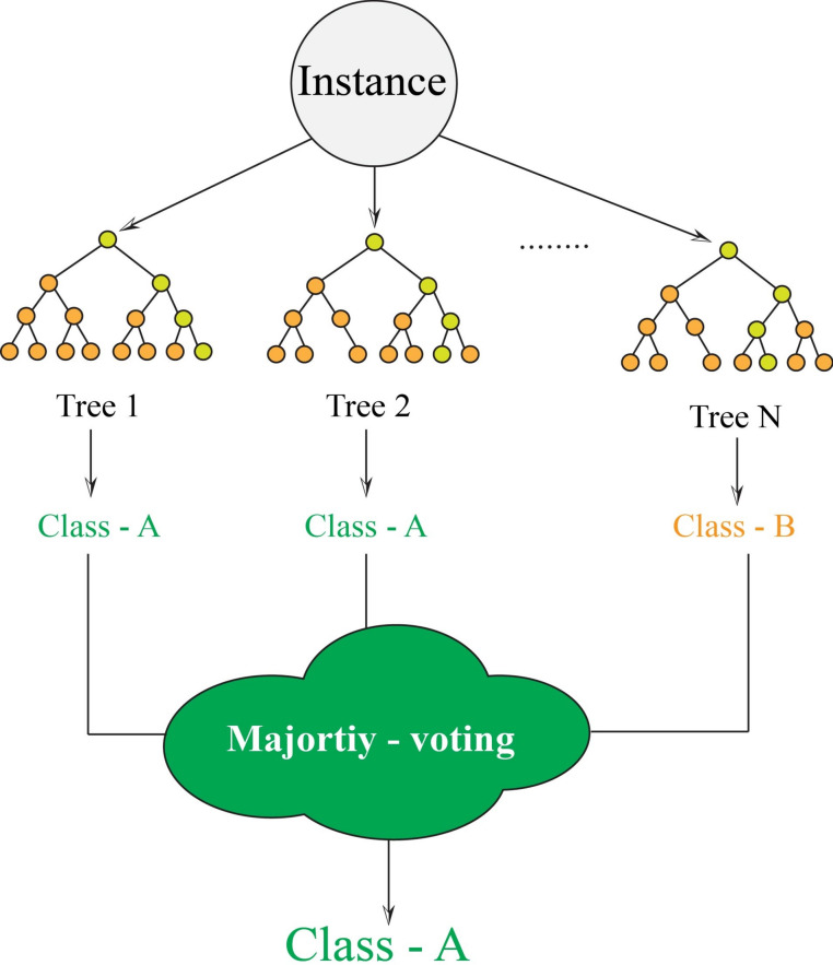
Random forest (RF) as a powerful decision tree ensemble first introduced by⁴⁷. It uses a collection of classification trees as its base learners. This approach has demonstrated its effectiveness in both classification and regression tasks, showing resilience against overfitting^48,49. Random forest applies bagging (bootstrap aggregating) and random subspace sampling to form a committee (Fig. 3). Moreover, random forest utilizes a diverse range of random trees, enhancing its effectiveness compared to conventional decision trees^50,51. Therefore, the ultimate classification label for each data instance is established by taking into account the majority opinion⁵². Moreover, random forest strategy chooses a random subset from the training data, allowing for duplicates, and utilizes this sampled data to undergo training. The outcome the framework can establish more accurate model by reducing the model variance. In addition, random forest utilizes the process of feature bagging, which it implies that only a selected set of features is employed for training phase. The interested readers can explore further information about random forest model within⁴⁷.

Fig. 3.

The random forest structure.

Gradient boosting

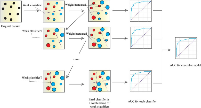
In this study, the classification of the response variable is carried out using Gradient Boosting model. Gradient Boosting is an amalgamation of boosting methods and decision tree paradigms to generate more accurate and resilient results⁵³ (Fig. 4). The primary benefit of Gradient Boosting is its superior computational efficiency and its increased capacity to deal with over-fitting issues⁵⁴. To enhance the accuracy of model, Gradient Boosting fits several decision trees⁵⁵. Therefore, for each new tree in the Gradient Boosting, the boosting technique is employed to choose a random group of all the data. In order to improve the chances of selecting data that was inadequately represented by earlier trees, the input data is assigned weights for every new tree in the model. To put it differently, once the initial tree has been fitted, the model will proceed to fit the second tree, taking into consideration the prediction error of previous tree, and continue this process iteratively. By considering the fit of trees that were constructed earlier, the model aims to improve its accuracy gradually⁵³. In fact, Gradient Boosting was developed to enhance the predictability of weak independent variables. Gradient descent is a commonly used technique in Gradient Boosting to build new trees that minimize difference between real and predicted values, and this strategy can be employed to forecast both continuous and discrete dependent variables. Friedman (2001)⁵³ provides a thorough explanation of the functioning of Gradient Boosting algorithm.

Fig. 4.

The gradient boosting structure.

Multilayer perceptron

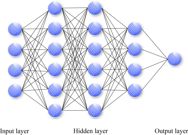
Multilayer perceptron (MLP) is a prevalent feed-forward artificial neural network architecture in the literature for classification tasks, with the back-propagation (BP) model being the most widely used^56,57. It should be noted that MLP model is a supervised learning strategy. The network is modeled after the neural system of the human brain and comprises processing elements known as neurons and connections⁵⁸. These neurons and connections are organized into three or more layers, including an input layer, one or more hidden layers, and an output layer⁵⁹ (Fig. 5). At the heart of MLP model are two primary components: the transformation of input parameters using a nonlinear operator called activation function to the output layer, followed by the back-propagation of classification difference between actual and estimated values to refine the process of weighting⁶⁰. The two procedures alternate cyclically until the error of model reaches a stable value. The formulation of the structure of a MLP model can be expressed as⁶¹:

7

where and p indicate output value and activation function. Also, w shows the connection weight that can be updated at each iteration. Moreover, the mathematical description of process of back-propagation can be shown as follows⁶²:

8

where w and are weights and the learning rate. Additionally, E and denote the prediction error energy and the parameter of momentum, respectively.

Fig. 5.

The schematic architecture of MLP.

Convolutional neural networks

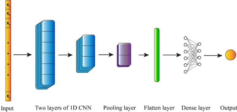
Convolutional neural network (CNN) is one of the popular types of neural network that is composed of a sequence of convolutional layers, pooling layers, and a fully connected layer⁶³ (Fig. 6). Although CNN was originally created for handling images, they have the capacity to be utilized for various data formats, including textual and auditory data. Convolutional layers utilize filters to analyze a portion of the input parameters and extract features from it⁶⁴. In the past few years, CNN have showcased remarkable capabilities in tackling a wide range of challenging issues. The primary concept behind CNN is that it can extract a hierarchical set of attributes that includes important features derived from insignificant features by using convolution. CNN can include as many convolutional layers as necessary⁶⁴. Increasing the number of convolutional layers allows for a greater extraction of resources. However, it also requires a higher amount of computational resources. Following a series of layers that involved convolution and pooling, the size of the input matrix was decreased, and intricate features were identified. Finally, when the feature map becomes adequately small, the contents are flattened into a vector of one dimension and then sent to a fully connected layer for further processing⁶⁴. In this study, the proposed 1D CNN architecture for binary classification begins with an input layer accepting data. The feature extraction stage consists of two convolutional layers: the first layer employs 48 filters with a kernel size of 2 and tanh activation, followed by a batch normalization layer to ensure training stability and faster convergence. The second convolutional layer contains 32 filters, also with kernel size 2, but utilizes ReLU activation, accompanied by a dropout layer (rate: 0.2) to prevent overfitting. A max pooling layer with pool size 2 is then applied to reduce the feature map dimensionality. The resulting feature maps are transformed into a vector representation through a flatten layer, which feeds into a fully connected dense layer of 32 neurons with ReLU activation. Another dropout layer with a higher rate of 0.5 is implemented before the final output layer, which consists of a single neuron with sigmoid activation for binary classification task.

Fig. 6.

The schematic architecture of CNN.

Dataset

The NCBI Gene Expression Omnibus (GEO) is a publicly accessible database where large amounts of gene expression data from various forms of high-throughput functional genomics, such as microarray and next-generation sequencing, are stored. The National Center for Biotechnology Information (NCBI) is responsible for maintaining the GEO database, which serves as a centralized location for researchers to store, search, and retrieve gene expression data.

The GEO database has a diverse collection of data from various species such as humans, rats, mice, and other model organisms. The sources of data in GEO are from research laboratories, state institutions, and companies. Researchers can use the GEO database to gain insights into gene expression patterns in various tissues, developmental stages, and disease conditions, making it a valuable resource. Access to GEO data is available through the NCBI website, which offers an easy-to-use interface for searching and downloading data. The NCBI portal can be searched for data based on different guidelines by researchers, such as type of tissue, species, study situation, and data type. Additionally, users can download raw data files for additional analysis or use the GEO2R tool for differential gene expression analysis. The database as a fundamental tool can be used for comprehension of patterns of gene expression and investigating their significance in health and disease. Its extensive assortment of high-throughput gene expression data from various species and experimental conditions attracts attentions as an imperative tool for scientists in life sciences. Therefore, in this study, for classifying CRC response to radiochemotherapy, the data (GSE45404) was extracted from the NCBI Gene Expression Comprehensive (GEO) web resource (https://www.ncbi.nlm.nih.gov/geo/) based on different ML models by considering the most applicable features that were obtained from feature selection tools. This dataset by applying gene expression analysis revealed a signature of differentially expressed genes associated with (CRC), distinguishing patients who responded to radiochemotherapy from those who did not respond⁶⁵. In this study, the data was split into a training set (80%) and a testing set (20%).

Results and discussion

CRC as one of the most common cancers that can be explained as major malignant tumors that affect human health seriously^66–70. Among the various feature selection techniques for CRC classification, Chi-Square, recursive feature elimination, f-classif, and mutual information and so on have been implemented frequently⁷¹.

In this research, classification of CRC response to radiochemotherapy was carried out utilizing three feature selection techniques including the mutual information, f-classif, and Chi-Square, respectively. Considering a two-class CRC classification labeling with positive (p) or negative (n), four possible issues from a CRC classification technique can be occurred. If the predictive issue is p and the observed issue is also p, then it is defined a true positive (TP); but, if the observed issue is n, then it is said to be a false positive (FP). However, a true negative (TN) is defined when the predictive issue and the observed issue are n, and false negative (FN) is defined when the predictive issue is n whereas the observed issue is p⁷². Also, three performance measures including accuracy (ACC, refer to Eq. 9), sensitivity (SN, refer to Eq. 10), and specificity (SP, refer to Eq. 11) were employing from the confusion matrix⁷³.

9

10

11

Mutual information technique

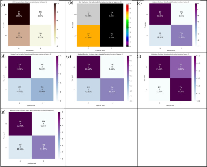
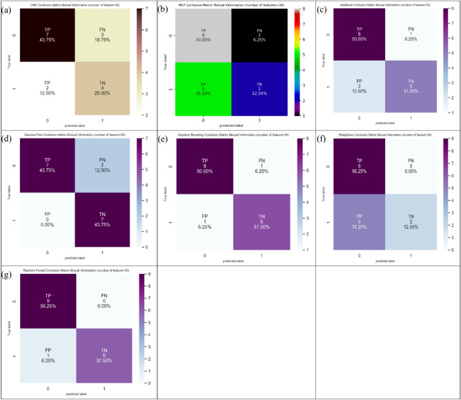
Mutual information (MI) technique can be defined as a special instance for the generalized quantity matching to distance measure between two probability mass functions^74–76. Table 1–4 present the comparison between the machine learning (ML) and deep learning (DL) models based on different feature selection techniques (i.e., mutual information, f-classif, and Chi-Square) for CRC classification by considering five, ten, twenty, and thirty features, respectively. Dependent on mutual information (MI) technique, it can be found from five features (Table 1) that Gradient Boosting gave the highest ACC (87.5%). In SN analysis, Gradient Boosting, MLP, and CNN provided the highest values (100%). Among seven ML and DL models, four models (i.e., KNeighbors, AdaBoost, random forest, and Gradient Boosting) showed the highest values (71.4%) in SP analysis. Figure 7 shows the confusion matrix for different ML and DL models of CRC classification based on selected top five features utilizing MI technique.

Table 1.

The comparison between models based on different feature selection methods for colorectal cancer classification by considering five features.

Models	Accuracy (%)			Sensitivity (%)			Specificity (%)			F1 score
	MI	F-classif	Chi2	MI	F-classif	Chi2	MI	F-classif	Chi2	MI	F-classif	Chi2
Decision Tree	68.8	62.5	56.3	77.8	100.0	66.7	57.1	14.3	42.9	0.683	0.531	0.557
K-nearest neighbors	62.5	81.3	50.0	55.6	100.0	77.8	71.4	57.1	14.3	0.612	0.80	0.445
AdaBoost	81.3	62.5	50.0	88.9	77.8	66.7	71.4	42.9	28.6	0.87	0.584	0.445
Random Forest	81.3	68.8	50.0	88.9	77.8	77.8	71.4	57.1	14.3	0.81	0.683	0.483
Gradient Boosting	87.5	62.5	56.3	100.0	66.7	66.7	71.4	57.1	42.9	0.87	0.625	0.405
MLP	56.3	62.5	56.3	100.0	77.8	100.0	0.0	42.9	0.0	0.40	0.612	0.405
CNN	68.8	75.0	56.3	100.0	100.0	50.0	16.7	33.3	66.7	0.60	0.708	0.567

Table 4.

The comparison between models based on different feature selection methods for colorectal cancer classification by considering thirty features.

Models	Accuracy (%)			Sensitivity (%)			Specificity (%)			F1 score
	MI	F-classif	Chi2	MI	F-classif	Chi2	MI	F-classif	Chi2	MI	F-classif	Chi2
Decision Tree	87.5	56.3	43.8	77.8	66.7	66.7	100.0	42.9	14.3	0.742	0.445	0.445
K-nearest neighbors	68.8	93.8	50.0	100.0	100.0	55.6	28.6	85.7	42.9	0.667	0.870	0.5
AdaBoost	81.3	75.0	56.3	88.9	88.9	66.7	71.4	57.1	42.9	0.810	0.625	0.534
Random Forest	93.8	68.8	56.3	100.0	100.0	100.0	85.7	28.6	0.0	0.870	0.531	0.439
Gradient Boosting	87.5	62.5	56.3	88.9	66.7	100.0	85.7	57.1	0.0	0.810	0.741	0.401
MLP	62.5	87.5	56.3	88.9	100.0	88.9	28.6	71.4	14.3	0.405	0.871	0.405
CNN	68.8	75.0	75.0	70.0	60.0	80.0	66.7	100.0	66.7	0.691	0.75	0.537

Fig. 7.

Confusion matrix for different AI models for colorectal cancer classification based on top five features selected using MI technique, a) CNN, b) MLP, c) Adaboost, d) Decision tree, e) Gradient boosting, f) Kneighbors, and, g) Random forest.

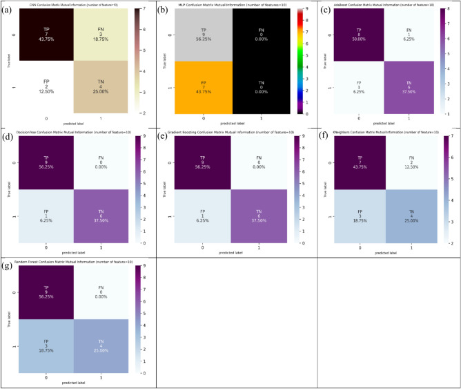
Considering ten features (Table 2) conditional on the MI technique, decision tree and Gradient Boosting provided the best values of 93.8% in ACC evaluation. Conditional on SN evaluation, decision tree, random forest, Gradient Boosting, and MLP gave the best values of 100.0%. Also, decision tree, AdaBoost, and Gradient Boosting represent the best values of 85.7% conditional on SP evaluation. Figure 8 shows the confusion matrix for different ML and DL models of CRC classification based on selected top ten features utilizing MI technique.

Table 2.

The comparison between models based on different feature selection methods for colorectal cancer classification by considering ten features.

Models	Accuracy (%)			Sensitivity (%)			Specificity (%)			F1 score
	MI	F-classif	Chi2	MI	F-classif	Chi2	MI	F-classif	Chi2	MI	F-classif	Chi2
Decision Tree	93.8	75.0	62.5	100.0	77.8	66.7	85.7	71.4	57.2	0.936	0.75	0.375
K-nearest neighbors	68.8	81.3	37.5	77.8	88.9	55.6	57.1	71.4	14.3	0.683	0.741	0.354
AdaBoost	87.5	81.3	56.3	88.9	77.8	100.0	85.7	85.7	0.0	0.741	0.741	0.439
Random Forest	81.3	75.0	56.3	100.0	77.8	100.0	57.1	71.4	0.0	0.80	0.722	0.375
Gradient Boosting	93.8	87.5	56.3	100.0	88.9	100.0	85.7	85.7	0.0	0.87	0.875	0.5
MLP	56.3	68.8	56.3	100.0	100.0	100.0	0.0	28.6	0.0	0.405	0.811	0.531
CNN	68.8	87.5	50.0	70.0	90.0	50.0	66.7	83.3	50.0	0.691	0.875	0.507

Fig. 8.

Confusion matrix for different AI models for colorectal cancer classification based on top ten features selected using MI technique, a) CNN, b) MLP, c) Adaboost, d) Decision tree, e) Gradient boosting, f) Kneighbors, and, g) Random forest.

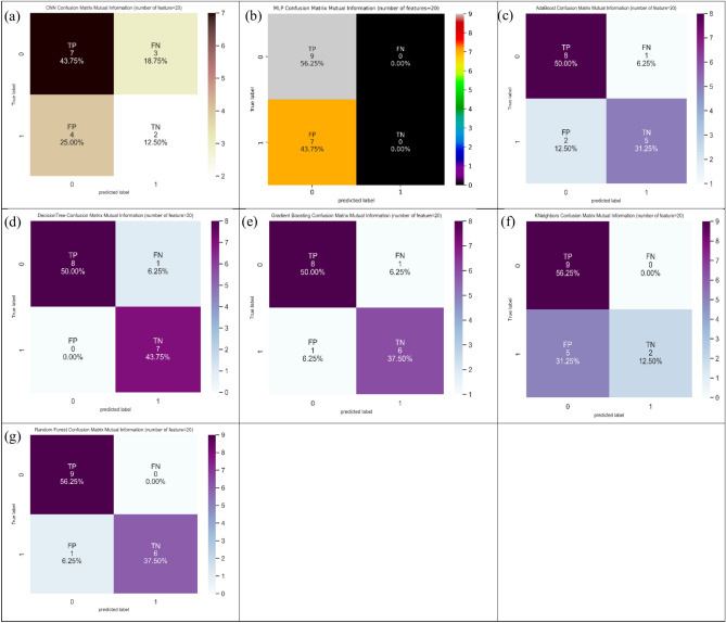
Twenty features (Table 3) provided the ACC, SN, and SP measures conditional on the MI technique. The ACC measure supplied the topmost value (93.8%) for decision tree and random forest. In addition, the SN measure yielded the topmost value (100%) for KNeighbors, random forest, and MLP. Also, the SP measure furnished the topmost value (100%) for decision tree. Figure 9 shows the confusion matrix for different ML and DL models of CRC classification based on selected top twenty features utilizing MI technique.

Table 3.

The comparison between models based on different feature selection methods for colorectal cancer classification by considering twenty features.

Models	Accuracy (%)			Sensitivity (%)			Specificity (%)			F1 score
	MI	F-classif	Chi2	MI	F-classif	Chi2	MI	F-classif	Chi2	MI	F-classif	Chi2
Decision Tree	93.8	62.5	56.3	88.9	77.8	88.9	100.0	42.9	14.3	0.667	0.5	0.531
K-nearest neighbors	68.8	81.3	37.5	100.0	88.9	55.6	28.6	71.4	14.3	0.534	0.810	0.306
AdaBoost	81.3	81.3	56.3	88.9	88.9	77.8	71.4	71.4	28.6	0.75	0.688	0.483
Random Forest	93.8	81.3	56.3	100.0	88.9	100.0	85.7	71.4	0.0	0.870	0.80	0.354
Gradient Boosting	87.5	75.0	50.0	88.9	88.9	66.7	85.7	57.1	28.6	0.741	0.741	0.5
MLP	56.3	81.3	62.5	100.0	88.9	100.0	0.0	71.4	14.3	0.405	0.810	0.45
CNN	56.3	87.5	43.8	70.0	90.0	30.0	33.3	83.3	66.7	0.553	0.875	0.426

Fig. 9.

Confusion matrix for different AI models for colorectal cancer classification based on top twenty features selected using MI technique, a) CNN, b) MLP, c) Adaboost, d) Decision tree, e) Gradient boosting, f) Kneighbors, and, g) Random forest.

Finally, regarding thirty features, random forest marked the maximum value of 93.8% in ACC indices, and two models including KNeighbors and random forest marked the maximum value of 100.0% in SN indices. Decision tree, furthermore, marked the maximum value of 100.0% in SP indices. Figure 10 shows the confusion matrix for different ML and DL models of CRC classification based on selected top thirty features utilizing MI technique.

Fig. 10.

Confusion matrix for different AI models for colorectal cancer classification based on top thirty features selected using MI technique, a) CNN, b) MLP, c) Adaboost, d) Decision tree, e) Gradient boosting, f) Kneighbors, and, g) Random forest.

F-classif technique

F-classif⁷⁷, one of univariate correlations, technique was implemented to count the features from the analysis dataset. The application of F-classif technique can be found from Tables 1–4 dependent on five, ten, twenty, and thirty features. Relying on f-classif technique, it can be judged from five features (Table 1) that KNeighbors produced the highest accuracy (81.3%) among the applied ML and DL models. In SN analysis, three ML models including decision tree, KNeighbors, and CNN gave the highest values (100%). Among the ML and DL models, three ML models (i.e., KNeighbors, random forest, and Gradient Boosting) showed the highest values (57.1%) in SP analysis. Figure 11 shows the confusion matrix for different ML and DL models of CRC classification based on selected top five features employing F-classif technique.

Fig. 11.

Confusion matrix for different AI models for colorectal cancer classification based on top five features selected using F-classif technique, a) CNN, b) MLP, c) Adaboost, d) Decision tree, e) Gradient boosting, f) Kneighbors, and, g) Random forest.

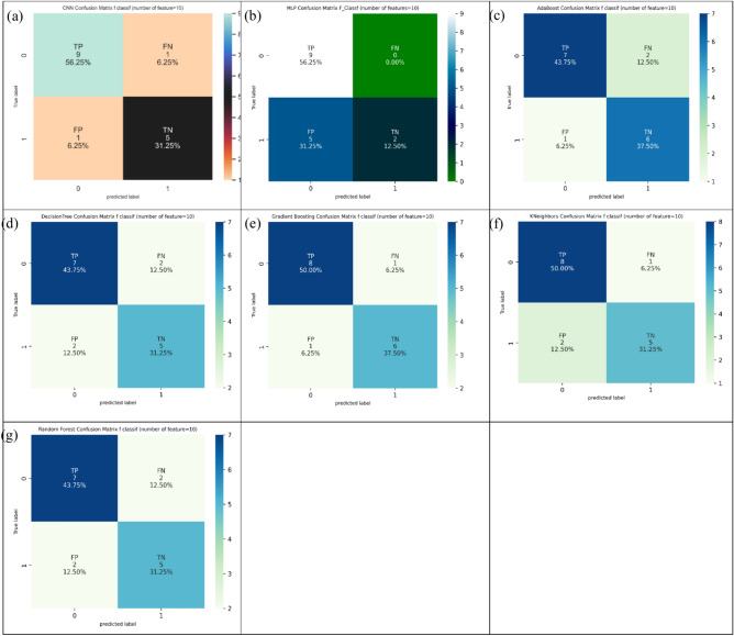
Recognizing ten features (Table 2) conditional on the F-classif technique, Gradient Boosting, and CNN supplied the best outputs of 87.5% in ACC assessment. Contemplating SN assessment, MLP furnished the best output of 100.0%. Also, AdaBoost and Gradient Boosting represented the best outputs of 85.7% based on SP assessment. Figure 12 shows the confusion matrix for different ML and DL models of CRC classification based on selected top ten features employing F-classif technique.

Fig. 12.

Confusion matrix for different AI models for colorectal cancer classification based on top ten features selected using F-classif technique, a) CNN, b) MLP, c) Adaboost, d) Decision tree, e) Gradient boosting, f) Kneighbors, and, g) Random forest.

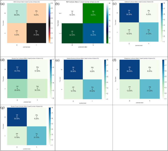
Twenty features from Table 3 supported the ACC, SN, and SP indices conditional on the F-classif technique. CNN furnished the top-class values of 87.5% (ACC), 90.0% (SN), and 83.3% (SP) among the ML and DL models. Figure 13 shows the confusion matrix for different ML and DL models of CRC classification based on selected top twenty features employing F-classif technique.

Fig. 13.

Confusion matrix for different AI models for colorectal cancer classification based on top twenty features selected using F-classif technique, a) CNN, b) MLP, c) Adaboost, d) Decision tree, e) Gradient boosting, f) Kneighbors, and, g) Random forest.

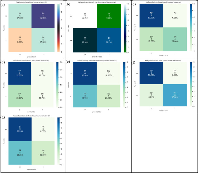
Lastly, considering thirty features (Table 4), KNeighbors showed the maximum value of 93.8% in ACC indices, and three models including KNeighbors, random forest, and MLP provided the maximum value of 100.0% in SN indices. In addition, CNN provided the maximum value of 100.0% in SP indices. Figure 14 shows the confusion matrix for different ML and DL models of CRC classification based on selected top thirty features employing F-classif technique.

Fig. 14.

Confusion matrix for different AI models for colorectal cancer classification based on top thirty features selected using F-classif technique, a) CNN, b) MLP, c) Adaboost, d) Decision tree, e) Gradient boosting, f) Kneighbors, and, g) Random forest.

Chi-Square technique

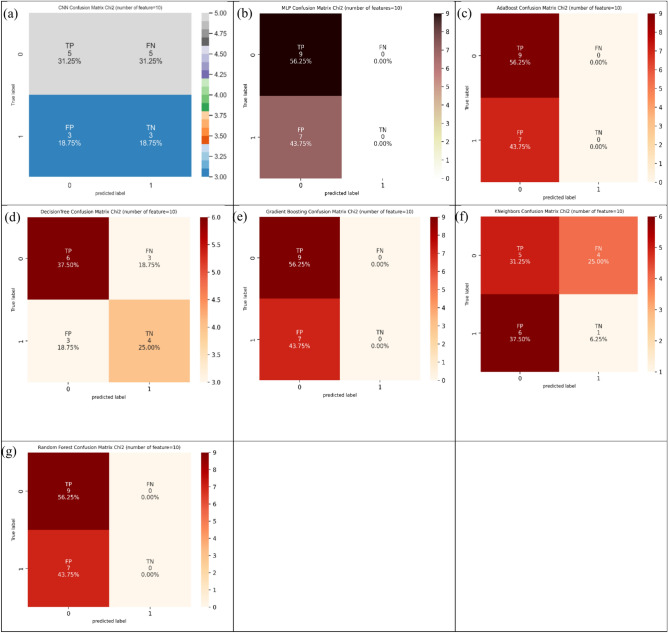
The definition of Chi-Square technique can be explained for finding the dependency between features and their labels on input and target dataset, and then selected top 30% of confusion matrix⁷¹. The application and employment of Chi-Square technique can be judged from Tables 1–4 based on five, ten, twenty, and thirty features. Conditional on Chi-Square technique, it can be assessed from five features (Table 1) that four models including decision tree, Gradient Boosting, MLP, and CNN suggested the highest values of 56.3% in ACC estimation. Also, MLP and CNN suggested the highest values of 100.0% and 66.6% in SN and SP estimation, respectively. Figure 15 represents the confusion matrix for different ML and DL models of CRC classification based on selected top five features hiring Chi-Square technique.

Fig. 15.

Confusion matrix for different AI models for colorectal cancer classification based on top five features selected using Chi-squared technique, a) CNN, b) MLP, c) Adaboost, d) Decision tree, e) Gradient boosting, f) Kneighbors, and, g) Random forest.

Identifying ten features (Table 2) dependent on the Chi-Square technique, decision tree represented the topmost output of 62.5% in ACC index. Noting SN index, among the applied ML and DL models, four models (i.e., AdaBoost, random forest, Gradient Boosting, and MLP) supplied the topmost outputs of 100.0% in SN index. Information for SP index demonstrated the topmost output of 57.2% in decision tree. Figure 16 represents the confusion matrix for different ML and DL models of CRC classification based on selected top ten features hiring Chi-Square technique.

Fig. 16.

Confusion matrix for different AI models for colorectal cancer classification based on top ten features selected using Chi-squared technique, a) CNN, b) MLP, c) Adaboost, d) Decision tree, e) Gradient boosting, f) Kneighbors, and, g) Random forest.

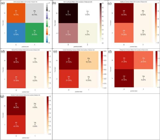
Table 3 demonstrated the topmost outputs of suggested indexes including ACC (62.5%) in MLP, SN (100.0%) in random forest and MLP, and SP (66.7%) in CNN. Figure 17 represents the confusion matrix for different ML and DL models of CRC classification based on selected top twenty features hiring Chi-Square technique.

Fig. 17.

Confusion matrix for different AI models for colorectal cancer classification based on top twenty features selected using Chi-squared technique, a) CNN, b) MLP, c) Adaboost, d) Decision tree, e) Gradient boosting, f) Kneighbors, and, g) Random forest.

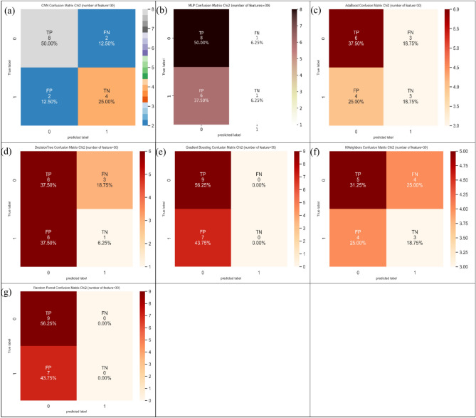
At last, it can be found from Table 4 that CNN furnished the largest value of 75.0% in ACC index, and two models (i.e., random forest and Gradient Boosting) supplied the largest value of 100.0% in SN index. Also, CNN produced the largest value of 66.7% in SP index. Figure 18 represents the confusion matrix for different ML and DP models of CRC classification based on selected top thirty features hiring Chi-Square technique.

Fig. 18.

Confusion matrix for different AI models for colorectal cancer classification based on top thirty features selected using Chi-squared technique, a) CNN, b) MLP, c) Adaboost, d) Decision tree, e) Gradient boosting, f) Kneighbors, and, g) Random Forest.

ROC curve

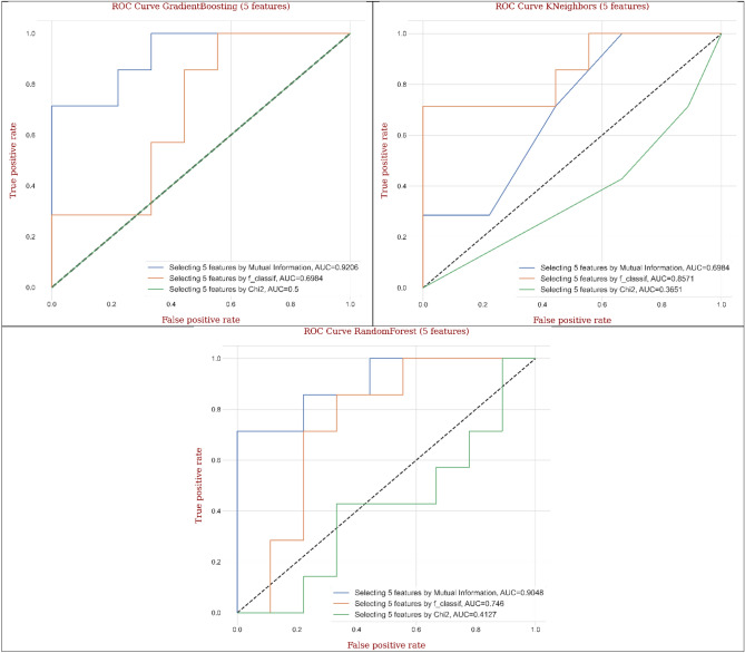
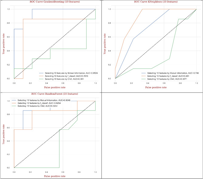
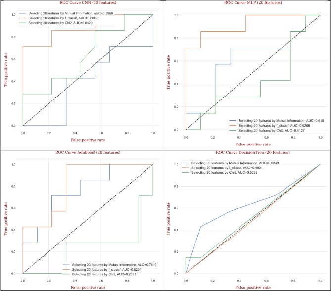
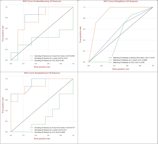
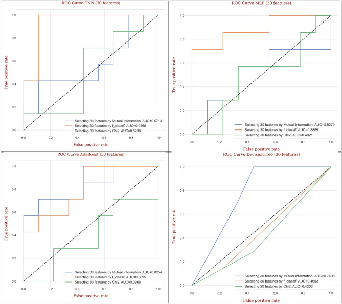
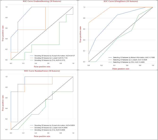
Receiver operating characteristic (ROC) curve can be described as a graphical scheme that demonstrates the diagnostic capacity of a binary classification system^72,78,79. Therefore, ROC curve can be designed by plotting the true positive rate (TPR) versus the false positive rate (FPR) conditional on the different threshold frameworks. The TPR is explained as sensitivity. Also, FRP can be computed as 1 minus specificity (1-specificity). ROC curve is one of useful methods to select optimized models and to abandon useless ones from the class distribution. In recent years, ROC curve can be employed in medical decision making, ML, and DL researches^80,81.

To compare the applied feature selection techniques, the performance of ROC can be reduced using a single value representing expected performance⁷⁸. Since the area under the ROC curve (AUC) value is a part of the unit square area, the addressed value will suggest from 0.00 to 1.00. Also, the realistic classification techniques cannot represent AUC value less than 0.50⁸². Figure 19 shows ROC curves generated from different ML and DL models for CRC classification by considering five features based on different feature selection techniques. In CNN, MLP, and KNeighbors, the values of AUC (i.e., 0.850, 0.794, and 0.857) employing F-classif technique had greater area and better performance in average compared to MI and Chi-Square techniques. Also, AdaBoost, decision tree, Gradient Boosting, random forest represented superior performance for the values of AUC (i.e., 0.989, 0.675, 0.825, and 0.878) employing MI techniques compared to F-classif and Chi-Square techniques. Conditional on the performances for the best ML and DL models, AdaBoost provided the highest AUC (0.989) utilizing MI technique, while decision tree supplied the lowest AUC (0.675) utilizing MI technique compared to other models.

Fig. 19.

The ROC curves generated from AI models for colorectal cancer classification based on different feature selection methods by considering five features.

Figure 20 illustrates ROC curves generated from different ML and DL models for CRC classification by considering ten features based on different feature selection techniques. The applied models including CNN, MLP, and KNeighbors showed the greatest values of AUC (0.900, 0.809, and 0.863) and excellent average performance employing F-classif technique compared to MI and Chi-Square techniques. In addition, AdaBoost, decision tree, Gradient Boosting, and random forest suggested the best values of AUC (0.984, 0.928, 0.968, and 0.952) and outstanding average performance applying MI technique compared to F-classif and Chi-Square techniques. Considering the achievements for the best ML and DL models, AdaBoost supplied the topmost AUC (0.984) utilizing MI technique, while MLP gave the lowest AUC (0.809) utilizing F-classif technique compared to other models.

Fig. 20.

The ROC curves generated from AI models for colorectal cancer classification based on different feature selection methods by considering ten features.

Figure 21 displays ROC curves generated from different ML and DL models for CRC classification by considering twenty features based on different feature selection techniques. The employed models such as decision tree, gradient boosting, and random forest arrayed the maximum AUC values (0.944, 0.958, and 0.980) and outstanding mean performance utilizing MI technique compared to F-classif and Chi-Square techniques. Besides, the outputs of CNN, MLP, AdaBoost, and KNeighbors implied the remarkable values of AUC (0.950, 0.905, 0.952, and 0.905) and superb mean performance engaging F-classif technique compared to MI and Chi-Square techniques. Relying on the outputs for the best ML and DL models, random forest gave the greatest AUC (0.980) utilizing MI technique, while MLP and KNeighbors provided the lowest AUC (0.905) utilizing F-classif technique compared to other models.

Fig. 21.

The ROC curves generated from AI models for colorectal cancer classification based on different feature selection methods by considering twenty features.

Figure 22 exhibits ROC curves generated from different ML and DL models for CRC classification by considering thirty features based on different feature selection techniques. The engaged models such as decision tree, Gradient Boosting, and random forest arranged the maximum AUC values (0.889, 0.896, and 0.992) and magnificent mean performance handling MI technique compared to F-classif and Chi-Square techniques. As well, the outputs of CNN, MLP, AdaBoost, and KNeighbors signified the satisfactory values of AUC (0.917, 0.917, 0.870, and 0.992) and superior performance utilizing F-classif technique compared to MI and Chi-Square techniques. Dependent on the accomplishment for the best ML and DL models, random forest gave the greatest AUC (0.992) utilizing MI technique, while AdaBoost supplied the lowest AUC (0.870) utilizing F-classif technique compared to other models.

Fig. 22.

The ROC curves generated from AI models for colorectal cancer classification based on different feature selection methods by considering thirty features.

Discussion

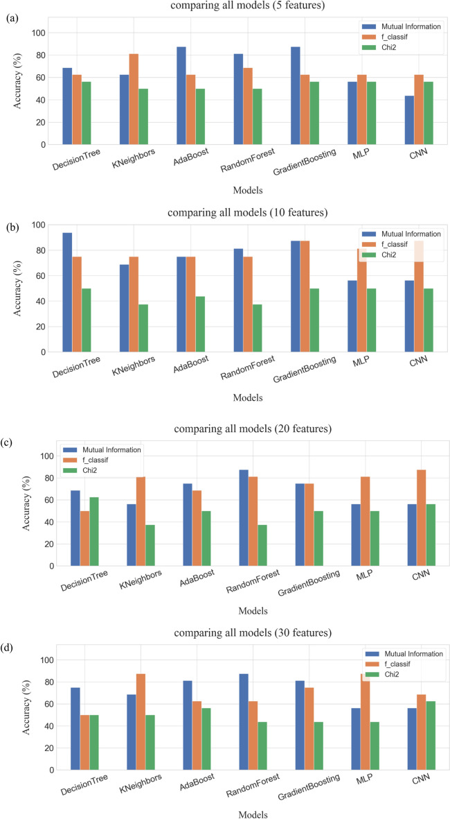
In this research, three feature selection techniques of binary classifier (i.e., MI, F-classif, and Chi-square) were applied for classifying colorectal cancer (CRC) response to radiochemotherapy. As well, three performance measures including accuracy (ACC), sensitivity (SN), and specificity (SP) were employed for evaluating of models’ classification based on five, ten, twenty, and thirty features, respectively. Also, ROC curve was utilized to compare the applied feature selection techniques and models. Figure 23(a)-(d) illustrates comparison of ACC (%) among ML and DL models utilizing the different feature selection techniques based on (a) five, (b) ten, (c) twenty, and (d) thirty features.

Fig. 23.

The comparison between AI models based on different feature selection methods, a) five features, b) ten features, c) twenty features, d) thirty features.

The results of ACC (Table 1 and Fig. 23a) and AUC (Fig. 19) utilizing MI technique supplied the highest values in decision tree (68.8% and 0.675), AdaBoost (81.3% and 0.989), random forest (81.3% and 0.878), and Gradient Boosting (87.5% and 0.825), where the first value = ACC (%) and the second value = AUC compared to F-classif and Chi-Square techniques conditional on the performance measures and ROC curve of five features. Also, F-classif technique provided the best results of ACC (%) and AUC for KNeighbors (81.3% and 0.857), MLP (62.5% and 0.794), and CNN (75.0% and 0.850) compared to MI and Chi-Square techniques. Chi-Square technique, however, didn’t supply the remarkable outputs in ACC (%) and AUC. As well, Gradient Boosting provided the best output in ACC (%), while AdaBoost supplied the best value in AUC among the applied feature selection techniques and models.

Dependent on the ten features in decision tree (93.8% and 0.928), AdaBoost (87.5% and 0.984), random forest (81.3% and 0.952), and Gradient Boosting (93.8% and 0.968), the results of ACC (Table 2 and Fig. 23b) and AUC (Fig. 20) utilizing MI technique provided the topmost values compared to F-classif and Chi-Square techniques. Besides, F-classif technique supported the best values of ACC (%) and AUC for KNeighbors (81.3% and 0.863), MLP (68.8% and 0.809), and CNN (87.5% and 0.900) compared to MI and Chi-Square techniques. However, Chi-Square technique couldn’t suggest the outstanding values in ACC (%) and AUC. Also, decision tree and Gradient Boosting presented the best outputs in ACC (%), while AdaBoost produced the best value in AUC among the applied feature selection techniques and models.

Relying on the twenty features in decision tree (93.8% and 0.944), random forest (93.8% and 0.980), and Gradient Boosting (87.5% and 0.958), the values of ACC (Table 3 and Fig. 23c) and AUC (Fig. 21) utilizing MI technique prepared the maximum values compared to F-classif and Chi-Square techniques. And, F-classif technique supported the best ones of ACC (%) and AUC for KNeighbors (81.3% and 0.905), MLP (81.3% and 0.905), and CNN (87.5% and 0.950) compared to MI and Chi-Square techniques. In case of AdaBoost, the ACC (%) gave the best one (81.3%) for MI and F-classif techniques. The significant differences, however, in AUC value were found between MI (0.778) and F-classif (0.952) techniques. In addition, decision tree and random forest demonstrated the leading outputs in ACC (%), whereas random forest supplied the outstanding value in AUC among the applied feature selection techniques and models.

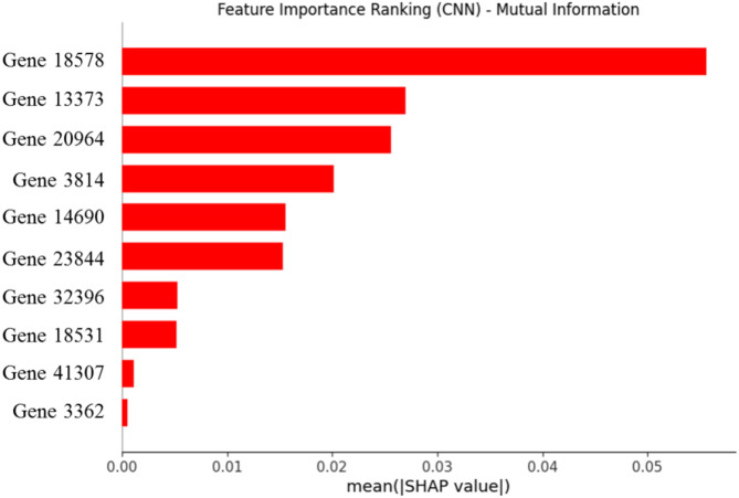
Based on the thirty features in decision tree (87.5% and 0.889), random forest (93.8% and 0.992), and Gradient Boosting (87.5% and 0.896), the outcomes of ACC (Table 4 and Fig. 23d) and AUC (Fig. 22) utilizing MI technique formed the highest values compared to F-classif and Chi-Square techniques. And, F-classif technique supplied the best outcomes of ACC (%) and AUC for KNeighbors (93.8% and 0.992), MLP (87.5% and 0.917), and CNN (75.0% and 0.917) compared to MI and Chi-Square techniques. However, the values of ACC (%) and AUC provided the different significances for MI (81.3% and 0.778) and F-classif (75.0% and 0.870) techniques employing AdaBoost. In addition, random forest and KNeighbors demonstrated the top outputs in ACC (%) and AUC among the applied feature selection techniques and models. Figure 24 shows the importance analysis of the most influential features identified using the MI feature selection method in the CNN model, which displays the main gene rankings.

Fig. 24.

SHAP results for identifying the importance of ten features selected using the MI method.

Searching for, in addition, the historic and similar articles and reports for classifying CRC response to radiochemotherapy conditional on the different artificial intelligence-based (e.g., ML and DL) models and feature selection techniques, Li et al. (2008)⁸³ applied three ML models utilizing two feature selection techniques to classify CRC. Results showed that SVM-PSO-GA supplied the best performance for classifying CRC with high accuracy. Zhang et al. (2009)⁸⁴ handled five ML models combined with GE hybrid feature selection technique for CRC classification. They explained that 7NN-GE hybrid gave the best performance for CRC classification accurately. Yang et al. (2010)⁸⁵ engaged three ML models based on two feature selection techniques for CRC classification. They found that 7NN-MF-GE provided the best accuracy compared with comparable ML models. Kulkarni et al. (2011)⁸⁶ compared two ML models utilizing two feature selection techniques for CRC classification. They investigated that GP-MI model was the most alternative approach for CRC classification. Al-Rajab et al. (2017)⁸⁷ utilized four ML models embedded with three feature selection techniques to classify CRC. Results demonstrated that SVM-PSO model surpassed the performance of CRC classification compared to suggested ML models. Salem et al. (2017)⁸⁸ implemented GP model based on two feature selection techniques for classifying CRC. They presented that GP-IG-SGA model improved the classification performance of CRC with high accuracy. Zhao et al. (2019)⁸⁹ developed five ML models with two feature selection and four SVM kernel selection techniques for classifying CRC. They provided that LR-SVM was the best model for classifying CRC. Also, Al-Rajab et al. (2021)⁹⁰ developed four ML models based on two-stage hybrid feature selection techniques for CRC classification. They explained that DT and KNN models provided the best classification of CRC based on image dataset.

However, the authors cannot find the same research to classify CRC based on different ML and DL models including DT, KNN, AdaBoost, RF, Gradient Boosting, MLP, and CNN from the previous literature. Also, this research can enhance the employment of ML and DL models for CRC classification and treatment plans of CRC patients. In addition, Table 5 suggests the previous researches for classifying CRC based on different artificial intelligence models and feature selection techniques.

Table 5.

The previous researches for classifying CRC based on artificial intelligence-based models and feature selection techniques.

References	Models		Feature selection techniques	ACC(%) of Best Model
	Machine learning	Deep learning
Li et al. (2008)83	SVM, NB, DT	-	PSO, GA	91.90
Zhang et al. (2009)84	DT, NB, 7NN, 3NN, RF		GE Hybrid	85.34
Yang et al. (2010)85	NB, 7NN, RF		MF, GE	75.07
Kulkarni et al. (2011)86	GP, DT	-	MI, TA	100.00
Al-Rajab et al. (2017)87	SVM, NB, DT, GP	-	PSO, GA, IG	94.00
Salem et al. (2017)88	GP	-	IG, SGA	85.48
Zhao et al. (2019)89	RF, NB, KNN, SVM, ANN	-	LR, ROC Curve	90.10
Al-Rajab et al. (2021)90	SVM, NB, DT, KNN	-	two-stage hybrid multifilter	93.75
This research (2024)	DT, KNN, AdaBoost, RF GB, MLP	CNN	MI, F-classif, Chi-Square	93.80

RF: Random Forest, SVM: Support Vector Machine, LR: Logistic Regression, MLP: Multi-layer Perceptron, NB: Naive Bayes, ACC: Accuracy, GP: Genetic Programing, TA: t-statistics, PSO: Particle Swarm Optimization, IG: Information Gain, GA: Genetic Algorithm, SGA: Standard Genetic Algorithm, 3NN: 3-Nearest Neighbor.

The limitation of this research can be explained as the introduction and application of different machine learning (i.e., DT, KNN, AdaBoost, RF, GB, and MLP) and deep learning (i.e., CNN) models to classify CRC response to radiochemotherapy based on the GEO dataset (GSE45404). Since an accurate classification of CRC has focused on specific artificial intelligence models and feature selection (i.e., MI, F-classif, and Chi-square) techniques, the current research for classifying CRC cannot supply the generalized evidence for diverse dataset (e.g., TCGA, UCI, and PICCOLO etc.). To boost the efficiency and accuracy of current research, therefore, diverse quality and quantity of dataset have to be utilized to cover the weakness and limitation of current research. Also, different machine learning, deep learning, and transfer learning (e.g., VGG16, VGG19, DenseNet169, and DenseNet201 etc.) are required to demonstrate the accurate classification of CRC response to radiochemotherapy. Therefore, the continuous researches by applying diverse dataset, unused feature selection techniques, different artificial intelligence models, and diverse optimization approaches are needed to improve the accuracy of CRC classification.

Conclusion

In this study, the performance several artificial intelligence models comprising of decision tree, K-nearest neighbors, adaboost, random forest, Gradient Boosting, multi-layer perceptron neural network, and convolutional neural network for classification of colorectal cancer response to radiochemotherapy was investigated. In the first step, models were trained and tested based on four different scenarios of features that were obtained using mutual information, F-classif, and Chi-Square methods. Moreover, the observed dataset was gathered from the NCBI Gene Expression Omnibus (GEO). The results obtained from outputs of models indicate that random forest, Gradient Boosting, decision tree, and K-nearest neighbors significantly improved the performance in terms of the accuracy indicator (93.8%.) of other models. According to this study, the proposed artificial intelligence models have the capacity to function as an efficient alternative in classification problems in medical applications. In order to address the constraints of artificial intelligence models and propose future research possibilities, classification of CRC response to radiochemotherapy can be enhanced through using optimization techniques such as particle swarm optimization, genetic algorithm, grey wolf algorithm methodologies to obtain the best hyperparameters of classifier models.

Author contributions

F.B.:Conceptualization, Supervision, Writing—Original Draft, Writing—Review & Editing. M. A.: Formal analysis, Data Curation, Project administration, Writing—Original Draft, Writing—Review & Editing. K.M.: Software, Writing—Original Draft. S.H.: Methodology, Writing—Original Draft. S.K.: Writing—Original Draft, Writing—Review & Editing. S.K.: Writing—Original Draft. M.S.: Writing—Original Draft. S.A.: Writing—Original Draft. A.T.: Writing—Original Draft.

Data availability

The data that support the findings of this study are available from the corresponding author.

Declarations

Competing interests

The authors declare no competing interests.

References

- 1.Dimitriou, N., Arandjelović, O., Harrison, D. J. & Caie, P. D. A principled machine learning framework improves accuracy of stage II colorectal cancer prognosis. NPJ Digit. Med.1(1), 52 (2018). [DOI] [PMC free article] [PubMed] [Google Scholar]
- 2.Xu, Y., Ju, L., Tong, J., Zhou, C.-M. & Yang, J.-J. Machine learning algorithms for predicting the recurrence of stage IV colorectal cancer after tumor resection. Sci. Rep.10(1), 2519 (2020). [DOI] [PMC free article] [PubMed] [Google Scholar]
- 3.Xi, Y. & Xu, P. Global colorectal cancer burden in 2020 and projections to 2040. Transl. Oncol.14(10), 101174 (2021). [DOI] [PMC free article] [PubMed] [Google Scholar]
- 4.Rawla, P., Sunkara, T. & Barsouk, A. Epidemiology of colorectal cancer: incidence, mortality, survival, and risk factors. Gastroenterol. Rev./Prz. Gastroenterol..14(2), 89–103 (2019). [DOI] [PMC free article] [PubMed] [Google Scholar]
- 5.Wan, N. et al. Machine learning enables detection of early-stage colorectal cancer by whole-genome sequencing of plasma cell-free DNA. BMC Cancer.19, 1–10 (2019). [DOI] [PMC free article] [PubMed] [Google Scholar]
- 6.Takamatsu, M. et al. Prediction of early colorectal cancer metastasis by machine learning using digital slide images. Comput. Methods Progr. Biomed.178, 155–161 (2019). [DOI] [PubMed] [Google Scholar]
- 7.Prosnitz, R. G. et al. Quality measures for the use of adjuvant chemotherapy and radiation therapy in patients with colorectal cancer: a systematic review. Cancer107(10), 2352–2360 (2006). [DOI] [PubMed] [Google Scholar]
- 8.Siegel, R. et al. Preoperative short-course radiotherapy versus combined radiochemotherapy in locally advanced rectal cancer: A multi-centre prospectively randomised study of the Berlin Cancer Society. BMC Cancer9, 1–6 (2009). [DOI] [PMC free article] [PubMed] [Google Scholar]
- 9.Almarzouki, H. Z. Deep-learning-based cancer profiles classification using gene expression data profile. J. Healthc. Eng.2022(1), 4715998 (2022). [DOI] [PMC free article] [PubMed] [Google Scholar]
- 10.Mostavi, M., Chiu, Y.-C., Huang, Y. & Chen, Y. Convolutional neural network models for cancer type prediction based on gene expression. BMC Med. Genom.13, 1–13 (2020). [DOI] [PMC free article] [PubMed] [Google Scholar]
- 11.Du, M. et al. Integrated multi-omics approach to distinct molecular characterization and classification of early-onset colorectal cancer. Cell Rep. Med.4(3), 100974 (2023). [DOI] [PMC free article] [PubMed] [Google Scholar]
- 12.Haj-Hassan, H. et al. Classifications of multispectral colorectal cancer tissues using convolution neural network. J. Pathol. Inform.8(1), 1 (2017). [DOI] [PMC free article] [PubMed] [Google Scholar]
- 13.Pal, A., Garain, U., Chandra, A., Chatterjee, R. & Senapati, S. Psoriasis skin biopsy image segmentation using deep convolutional neural network. Comput. Methods Progr. Biomed.159, 59–69 (2018). [DOI] [PubMed] [Google Scholar]
- 14.George, K., Faziludeen, S. & Sankaran, P. Breast cancer detection from biopsy images using nucleus guided transfer learning and belief based fusion. Comput. Biol. Med.124, 103954 (2020). [DOI] [PubMed] [Google Scholar]
- 15.Srivastava, G., Chauhan, A. & Pradhan, N. Cjt-deo: Condorcet’s jury theorem and differential evolution optimization based ensemble of deep neural networks for pulmonary and colorectal cancer classification. Appl. Soft Comput.132, 109872 (2023). [Google Scholar]
- 16.Bychkov, D. et al. Deep learning based tissue analysis predicts outcome in colorectal cancer. Sci. Rep.8(1), 3395 (2018). [DOI] [PMC free article] [PubMed] [Google Scholar]
- 17.Li, J., Wang, P., Zhou, Y., Liang, H. & Luan, K. Different machine learning and deep learning methods for the classification of colorectal cancer lymph node metastasis images. Front. Bioeng. Biotechnol.8, 620257 (2021). [DOI] [PMC free article] [PubMed] [Google Scholar]
- 18.Nazari, E., Aghemiri, M., Avan, A., Mehrabian, A. & Tabesh, H. Machine learning approaches for classification of colorectal cancer with and without feature selection method on microarray data. Gene Rep.25, 101419 (2021). [Google Scholar]
- 19.Escorcia-Gutierrez, J. et al. Galactic swarm optimization with deep transfer learning driven colorectal cancer classification for image guided intervention. Comput. Electr. Eng.104, 108462 (2022). [Google Scholar]
- 20.Gao, Y., Zhu, Z. & Sun, F. Increasing prediction performance of colorectal cancer disease status using random forests classification based on metagenomic shotgun sequencing data. Synth. Syst. biotechnol.7(1), 574–585 (2022). [DOI] [PMC free article] [PubMed] [Google Scholar]
- 21.Li, Z., Sun, Y., An, F., Chen, H. & Liao, J. Self-supervised clustering analysis of colorectal cancer biomarkers based on multi-scale whole slides image and mass spectrometry imaging fused images. Talanta.263, 124727 (2023). [DOI] [PubMed] [Google Scholar]
- 22.Xu, H. et al. Classification of colorectal cancer consensus molecular subtypes using attention-based multi-instance learning network on whole-slide images. Acta Histochem.125(6), 152057 (2023). [DOI] [PubMed] [Google Scholar]
- 23.Zhou, C. et al. Histopathology classification and localization of colorectal cancer using global labels by weakly supervised deep learning. Comput. Med. Imaging Gr.88, 101861 (2021). [DOI] [PubMed] [Google Scholar]
- 24.Lo, C.-M. et al. Modeling the survival of colorectal cancer patients based on colonoscopic features in a feature ensemble vision transformer. Comput. Med. Imaging Gr.107, 102242 (2023). [DOI] [PubMed] [Google Scholar]
- 25.Schirris, Y., Gavves, E., Nederlof, I., Horlings, H. M. & Teuwen, J. DeepSMILE: Contrastive self-supervised pre-training benefits MSI and HRD classification directly from H&E whole-slide images in colorectal and breast cancer. Med. Image Anal.79, 102464 (2022). [DOI] [PubMed] [Google Scholar]
- 26.Raghav, S. et al. A hierarchical clustering approach for colorectal cancer molecular subtypes identification from gene expression data. Intell. Med.4(1), 43–51 (2024). [Google Scholar]
- 27.Chang, X. et al. Predicting colorectal cancer microsatellite instability with a self-attention-enabled convolutional neural network. Cell Rep. Med.4(2), 100914 (2023). [DOI] [PMC free article] [PubMed] [Google Scholar]
- 28.Luo, R. & Bocklitz, T. A systematic study of transfer learning for colorectal cancer detection. Inform. Med. Unlocked.40, 101292 (2023). [Google Scholar]
- 29.Kumar, A., Vishwakarma, A. & Bajaj, V. Crccn-net: Automated framework for classification of colorectal tissue using histopathological images. Biomed. Signal Process. Control.79, 104172 (2023). [Google Scholar]
- 30.Arowolo, M. O., Aigbogun, H. E., Michael, P. E., Adebiyi, M. O. & Tyagi, A. K. A predictive model for classifying colorectal cancer using principal component analysis 205–216 (Elsevier, 2023). [Google Scholar]
- 31.Parhami, P., Fateh, M., Rezvani, M. & Alinejad-Rokny, H. A comparison of deep neural network models for cluster cancer patients through somatic point mutations. J. Ambient Intell. Humaniz. Comput.14(8), 10883–10898 (2023). [Google Scholar]
- 32.Kim, S.-H., Koh, H. M. & Lee, B.-D. Classification of colorectal cancer in histological images using deep neural networks: An investigation. Multimed. Tools Appl.80(28), 35941–35953 (2021). [Google Scholar]
- 33.Su, Y. et al. Colon cancer diagnosis and staging classification based on machine learning and bioinformatics analysis. Comput. Boil. Med.145, 105409 (2022). [DOI] [PubMed] [Google Scholar]
- 34.Wang, T. et al. scMultiGAN: Cell-specific imputation for single-cell transcriptomes with multiple deep generative adversarial networks. Brief. Bioinform.10.1093/bib/bbad384 (2023). [DOI] [PMC free article] [PubMed] [Google Scholar]
- 35.Wang, T. et al. Accurately deciphering spatial domains for spatially resolved transcriptomics with stCluster. Brief. Bioinform.10.1093/bioinformatics/btac837 (2024). [DOI] [PMC free article] [PubMed] [Google Scholar]
- 36.Wang, T. et al. DFinder: A novel end-to-end graph embedding-based method to identify drug–food interactions. Bioinformatics10.1093/bioinformatics/btac837 (2023). [DOI] [PMC free article] [PubMed] [Google Scholar]
- 37.Wang, T. et al. Enhancing discoveries of molecular QTL studies with small sample size using summary statistic imputation. Brief. Bioinform.10.1093/bib/bbab370 (2022). [DOI] [PubMed] [Google Scholar]
- 38.Wang, T. et al. Exploring causal effects of sarcopenia on risk and progression of Parkinson disease by Mendelian randomization. npj Parkinson’s Dis.10(1), 164 (2024). [DOI] [PMC free article] [PubMed] [Google Scholar]
- 39.Wang, T. et al. PostGWAS: A web server for deciphering the causality post the genome-wide association studies. Comput. Biol. Med.171, 108108 (2024). [DOI] [PubMed] [Google Scholar]
- 40.VOSviewer version 1.6.20. (Leiden University, 2024).
- 41.Kotsiantis, S. B. Decision trees: A recent overview. Artif Intell. Rev.39, 261–283 (2013). [Google Scholar]
- 42.Yeon, Y.-K., Han, J.-G. & Ryu, K. H. Landslide susceptibility mapping in Injae, Korea, using a decision tree. Eng. Geol.116(3–4), 274–283 (2010). [Google Scholar]
- 43.Mitchell, T. M. & Mitchell, T. M. Machine learning (McGraw-hill, New York, 1997). [Google Scholar]
- 44.Freund, Y. & Schapire, R. E. A decision-theoretic generalization of on-line learning and an application to boosting. J. comput. Syst. Sci.55(1), 119–139 (1997). [Google Scholar]
- 45.Alizamir, M. et al. Developing an efficient explainable artificial intelligence approach for accurate reverse osmosis desalination plant performance prediction: Application of SHAP analysis. Eng. Appl. Comput. Fluid Mech.18(1), 2422060 (2024). [Google Scholar]
- 46.Hastie, T., Tibshirani, R., Friedman, J. & Franklin, J. The elements of statistical learning: data mining, inference and prediction. Math. Intell.27(2), 83–85 (2005). [Google Scholar]
- 47.Breiman, L. Random forests. Mach. learn.45, 5–32 (2001). [Google Scholar]
- 48.Rodriguez-Galiano, V. F., Ghimire, B., Rogan, J., Chica-Olmo, M. & Rigol-Sanchez, J. P. An assessment of the effectiveness of a random forest classifier for land-cover classification. ISPRS J. Photogram. Remote Sensing.67, 93–104 (2012). [Google Scholar]
- 49.Alizamir, M., Gholampour, A., Kim, S., Keshtegar, B. & Jung, W.-t. Designing a reliable machine learning system for accurately estimating the ultimate condition of FRP-confined concrete. Sci. Rep.14(1), 20466 (2024). [DOI] [PMC free article] [PubMed] [Google Scholar]
- 50.Dang, V.-H., Dieu, T. B., Tran, X.-L. & Hoang, N.-D. Enhancing the accuracy of rainfall-induced landslide prediction along mountain roads with a GIS-based random forest classifier. Bull. Eng. Geol. Environ.78, 2835–2849 (2019). [Google Scholar]
- 51.Alizamir, M., Heddam, S., Kim, S. & Mehr, A. D. On the implementation of a novel data-intelligence model based on extreme learning machine optimized by bat algorithm for estimating daily chlorophyll-a concentration: Case studies of river and lake in USA. J. Clean. Prod.285, 124868 (2021). [Google Scholar]
- 52.Alizamir, M. et al. Modelling daily soil temperature by hydro-meteorological data at different depths using a novel data-intelligence model: Deep echo state network model. Artif. Intell. Rev.54, 2863–2890 (2021). [Google Scholar]
- 53.Friedman, J. H. Greedy function approximation: A gradient boosting machine. Ann. Stat.29, 1189–1232 (2001). [Google Scholar]
- 54.Bentéjac, C., Csörgő, A. & Martínez-Muñoz, G. A comparative analysis of gradient boosting algorithms. Artif. Intell. Rev.54, 1937–1967 (2021). [Google Scholar]
- 55.Alizamir, M., Kim, S., Kisi, O. & Zounemat-Kermani, M. A comparative study of several machine learning based non-linear regression methods in estimating solar radiation: Case studies of the USA and Turkey regions. Energy.197, 117239 (2020). [Google Scholar]
- 56.Alizamir, M., Kisi, O., Kim, S. & Heddam, S. A novel method for lake level prediction: Deep echo state network. Arab. J. Geosci.13, 1–18 (2020). [Google Scholar]
- 57.Alizamir, M. et al. Improving the accuracy of daily solar radiation prediction by climatic data using an efficient hybrid deep learning model: Long short-term memory (LSTM) network coupled with wavelet transform. Eng. Appl. Artif. Intell.123, 106199 (2023). [Google Scholar]
- 58.Alizamir, M. et al. Prediction of daily chlorophyll-a concentration in rivers by water quality parameters using an efficient data-driven model: Online sequential extreme learning machine. Acta Geophys.69, 2339–2361 (2021). [Google Scholar]
- 59.Kisi, O. & Alizamir, M. Modelling reference evapotranspiration using a new wavelet conjunction heuristic method: Wavelet extreme learning machine vs wavelet neural networks. Agric. For. Meteorol.263, 41–48 (2018). [Google Scholar]
- 60.Alizamir, M. et al. Investigating landfill leachate and groundwater quality prediction using a robust integrated artificial intelligence model: Grey wolf metaheuristic optimization algorithm and extreme learning machine. Water.15(13), 2453 (2023). [Google Scholar]
- 61.Heidari, E., Sobati, M. A. & Movahedirad, S. Accurate prediction of nanofluid viscosity using a multilayer perceptron artificial neural network (MLP-ANN). Chemom. Intel. Lab. syst.155, 73–85 (2016). [Google Scholar]
- 62.LeCun, Y., Touresky, D., Hinton, G., Sejnowski, T. (ed.) A theoretical framework for back-propagation. In Proceedings of the 1988 connectionist models summer school (1988).
- 63.LeCun, Y. & Bengio, Y. Convolutional networks for images, speech, and time series. Handb. Brain Theory Neur. Netw.3361(10), 1995 (1995). [Google Scholar]
- 64.Thenmozhi, K. & Reddy, U. S. Crop pest classification based on deep convolutional neural network and transfer learning. Comput. Electron. Agric.164, 104906 (2019). [Google Scholar]
- 65.Agostini, M. et al. A functional biological network centered on XRCC3: A new possible marker of chemoradiotherapy resistance in rectal cancer patients. Cancer Biol. ther.16(8), 1160–1171 (2015). [DOI] [PMC free article] [PubMed] [Google Scholar]
- 66.Boyle, P. & Langman, M. J. ABC of colorectal cancer: Epidemiology. Bmj321((Suppl S6)), 0012452 (2000). [DOI] [PMC free article] [PubMed] [Google Scholar]
- 67.Parkin, D. M. International variation. Oncogene.23(38), 6329–6340 (2004). [DOI] [PubMed] [Google Scholar]
- 68.Moradi, A. et al. Survival of colorectal cancer in Iran. Asian Pac J. Cancer Prev.10(4), 583–586 (2009). [PubMed] [Google Scholar]
- 69.Ai, D. et al. Using decision tree aggregation with random forest model to identify gut microbes associated with colorectal cancer. Genes.10(2), 112 (2019). [DOI] [PMC free article] [PubMed] [Google Scholar]
- 70.Cai, D. et al. A metabolism-related radiomics signature for predicting the prognosis of colorectal cancer. Front. Mol. Biosci.7, 613918 (2021). [DOI] [PMC free article] [PubMed] [Google Scholar]
- 71.Ansari, A.A., Iqbal, A., Sahoo, B. (eds.) Heterogeneous defect prediction using ensemble learning technique. In Artificial intelligence and evolutionary computations in engineering systems (Springer, 2020).
- 72.Abbas, A., Abdelsamea, M. M. & Gaber, M. M. Detrac: Transfer learning of class decomposed medical images in convolutional neural networks. IEEE Access.8, 74901–74913 (2020). [Google Scholar]
- 73.Azzawi, H., Hou, J., Xiang, Y. & Alanni, R. Lung cancer prediction from microarray data by gene expression programming. IET Syst. Biol.10(5), 168–178 (2016). [DOI] [PMC free article] [PubMed] [Google Scholar]
- 74.Cover, T. M. Elements of information theory (John Wiley & Sons, 1999). [Google Scholar]
- 75.Kraskov, A., Stögbauer, H. & Grassberger, P. Estimating mutual information. Phys. Rev. E––Stat. Nonlinear Soft Matter Phys.69(6), 066138 (2004). [DOI] [PubMed] [Google Scholar]
- 76.Fan, X.-N., Zhang, S.-W., Zhang, S.-Y., Zhu, K. & Lu, S. Prediction of lncRNA-disease associations by integrating diverse heterogeneous information sources with RWR algorithm and positive pointwise mutual information. BMC Bioinform.20, 1–12 (2019). [DOI] [PMC free article] [PubMed] [Google Scholar]
- 77.Fux, A. et al. Objective video-based assessment of ADHD-like canine behavior using machine learning. Animals.11(10), 2806 (2021). [DOI] [PMC free article] [PubMed] [Google Scholar]
- 78.Fawcett, T. An introduction to ROC analysis. Pattern Recognit. Lett.27(8), 861–874 (2006). [Google Scholar]
- 79.Ahn, J. H. et al. Development of a novel prognostic model for predicting lymph node metastasis in early colorectal cancer: Analysis based on the surveillance, epidemiology, and end results database. Front. Oncol.11, 614398 (2021). [DOI] [PMC free article] [PubMed] [Google Scholar]
- 80.Masud, M., Sikder, N., Nahid, A.-A., Bairagi, A. K. & AlZain, M. A. A machine learning approach to diagnosing lung and colon cancer using a deep learning-based classification framework. Sensors.21(3), 748 (2021). [DOI] [PMC free article] [PubMed] [Google Scholar]
- 81.Yang, T. et al. Intelligent imaging technology in diagnosis of colorectal cancer using deep learning. IEEE Access.7, 178839–178847 (2019). [Google Scholar]
- 82.Hanley, J. A. & McNeil, B. J. The meaning and use of the area under a receiver operating characteristic (ROC) curve. Radiology.143(1), 29–36 (1982). [DOI] [PubMed] [Google Scholar]
- 83.Li, S., Wu, X. & Tan, M. Gene selection using hybrid particle swarm optimization and genetic algorithm. Soft Comput.12, 1039–1048 (2008). [Google Scholar]
- 84.Zhang, Z., Yang, P., Wu, X. & Zhang, C. An agent-based hybrid system for microarray data analysis. IEEE Intell. Syst.24(5), 53–63 (2009). [Google Scholar]
- 85.Yang, P., Zhou, B. B., Zhang, Z. & Zomaya, A. Y. A multi-filter enhanced genetic ensemble system for gene selection and sample classification of microarray data. BMC Bioinform.11, 1–12 (2010). [DOI] [PMC free article] [PubMed] [Google Scholar]
- 86.Kulkarni, A., Kumar, B. N., Ravi, V. & Murthy, U. S. Colon cancer prediction with genetics profiles using evolutionary techniques. Expert Syst. Appl.38(3), 2752–2757 (2011). [Google Scholar]
- 87.Al-Rajab, M., Lu, J. & Xu, Q. Examining applying high performance genetic data feature selection and classification algorithms for colon cancer diagnosis. Comput. Methods Progr. Biomed.146, 11–24 (2017). [DOI] [PubMed] [Google Scholar]
- 88.Salem, H., Attiya, G. & El-Fishawy, N. Classification of human cancer diseases by gene expression profiles. Appl. Soft Comput.50, 124–134 (2017). [Google Scholar]
- 89.Zhao, D. et al. A reliable method for colorectal cancer prediction based on feature selection and support vector machine. Med. Boil. Eng. Comput.57, 901–912 (2019). [DOI] [PubMed] [Google Scholar]
- 90.Al-Rajab, M., Lu, J. & Xu, Q. A framework model using multifilter feature selection to enhance colon cancer classification. Plos One.16(4), e0249094 (2021). [DOI] [PMC free article] [PubMed] [Google Scholar]
Associated Data
This section collects any data citations, data availability statements, or supplementary materials included in this article.
Data Availability Statement