Neural network-based aeroelastic system identification for predicting flutter of high flexibility wings

Abstract

Flutter is an extremely significant academic topic in both aerodynamics and aircraft design. Since flutter can cause multiple types of phenomena including bifurcation, period doubling, and chaos, it becomes one of the most unpredictable instability phenomena. The complexity of modeling aeroelasticity of high flexibility wings will be substantially simplified by investigating the prospect of system identification techniques to forecast flutter velocity. Therefore, a novel neural network (NN)-based method for aeroelastic system identification is proposed. The proposed NN-based approach constructs an NN framework of high flexibility wings flutter models with different materials and sizes, which can effectively predict the flutter velocity of flexible wings. The accuracy of the method is demonstrated by comparing with the simulation results.

Introduction

Wing flutter is a form of self-excited vibration with non-attenuated amplitude generated by an interaction of aerodynamic force, elastic restoring force, and inertial force^1–3. Wing flutter will happen when the flying velocity exceeds a particular number, recognized as the “flutter velocity”. The amplitude of vibration and the dynamic stress within the structure can simultaneously grow dramatically when the wing achieves flutter, leading to the rapid disintegration of aircrafts and the eventual annihilation of structures⁴. Thus, any kind of flutter is prohibited inside the intended flight envelope⁵. Flutter investigating is presently conducted using essentially three methods: theoretical calculations⁶, wind tunnel tests⁷, and flutter flight tests^8,9. Flutter flight tests and wind tunnel tests are both potentially dangerous and demand an enormous amount of labor and materials. In order to decrease the cycle and cost of flutter flight tests as well as their associated risks, it is crucial to propose a productive, affordable, and relatively low-risk flutter anticipation approach¹⁰. A significant subject in aeroelastic analysis, flight tests, and flutter airworthiness certification is how to accurately forecast the wing’s flutter characteristics throughout the flight envelope^11–13. Contemporary civil aircraft and high-altitude solar-powered aircraft are heavily reliant on composite materials with the development of technology. For example, the Boeing 787, which uses composite materials, has the characteristics of light weight, high chord ratio and high flexibility. Therefore, developing a method to forecast the high flexibility wings’ flutter velocity is crucial in the present scenario.

High flexibility wings indicate the aircraft wings’ exceptional bending and flexibility. In contrast to conventional aircraft wings, high flexibility wings utilizes more flexible materials and design, allowing for increased bending or deformation during flight^14,15. Furthermore, the aircraft mode will be dense given the high flexibility wings, which will complicate the flutter coupling relationship¹⁶. Consequently, one of the main factors influencing the flutter design of high aircraft will be the wings’ great degree of flexibility. One of the main methods for studying flutter velocity is nonlinear reduced-order models^17,18. Huang et al.¹⁹. applied the nonlinear reduced-order model to the transonic flutter analysis of the Isogai wing model accurately and efficiently. The application of control methods to solve structural problems has gained popularity in recent years due to advancements in modern control theory. One of the key subfields of system identification technology²⁰ is the estimation of key parameters, which defines the behavior of the system and the determination of the mathematical model of the system behavior based on the input and output time function of the system. The research on the ability of system identification technology to predict flutter velocity can provide some guidance on aeroelastic difficulties with high flexible wings.

In recent years, data-driven machine learning approaches have provided effective approaches to solve many problems in multidisciplinary fields. As an important method in the field of machine learning, neural network (NN) model is widely used in many fields such as identification of aeroelastic systems because of its powerful nonlinear fitting ability. For example, NASA Langley Laboratory and Boeing Company cooperatively carried out the aeroelastic response adaptive neural control (ANCAR)²¹ project. In their work, three different NN models were employed to obtain the flutter control rate, predictive control, and inverse model adjustment. In a transonic wind tunnel, the NACA0012 airfoil model was used to assess the control system, which demonstrated that the three-network adaptive control system can lessen wing model flutter in linear circumstances. Mattaboni and Quaranta²² used two feedforward NN models to control the flutter of the X-DIA model. They used a high number of theoretical data to train the network and extended the flight envelope by 15% when the flight envelope was uncontrolled. Pitt and Haudrich²³ designed an NN architecture for the plug-in of small-aspect-ratio fighters. The network was trained with the mass and moment of inertia of the station nodes as input and the flutter velocity as output. The results showed that the network can predict the flutter velocity caused by additional plug. This method was also used to predict the new flutter velocity that changes due to the weight increasing or decreasing of the wing during the maintenance of a low aspect ratio fighter²⁴. Mu et al.²⁵ proposed novel approach of machine learning-based control law for the problem of active flutter suppression, which is efficient and effective in expanding the flutter boundaries. Based on the above, we apply neural networks to predicting flutter of high flexibility wings, so as to develop an efficient and accurate aeroelastic system identification approach.

Many existing studies usually focus on the flutter characteristics of wings with a single material or geometric size, while this paper analyzes the flutter characteristics by expanding to a variety of materials and sizes. Specifically, the neural network is trained by the flutter characteristic data, and the neural network flutter model of the flexible wing with metal materials, composite materials and geometric dimensions is established. The trained neural network is used to predict the flutter speed, and the flutter characteristics obtained by simulation are compared to verify the correctness of the method. It provides important support for the design, optimization and safety assessment of highly flexible wings in the aerospace field, and promotes the progress of technology in this field.

The rest of this paper is organized as follows. Section "High flexibility wings dynamics and flutter analysis" introduces the modeling and simulation of flutter velocity. The system identification and NN algorithm are introduced in "The architecture of neural networks" Sect.. "NN training for high flexibility wings flutter" Section establishes the NN models of metallic materials, composite materials, and the same materials with different geometric sizes of high flexibility wings. In "Predicting results of high flexibility wings’ flutter" Sect., the trained NN is used to predict the unknown flutter velocity of the high flexibility wing model. Conclusions are summarized in "Conclusion"Sect.

High flexibility wings dynamics and flutter analysis

Structural modeling based on plate model

The establishment of flutter model includes structural modeling and aerodynamic modeling. Structural modeling is generally based on beam model, plate model and solid structure model. The aerodynamic model generally simplifies the wing surface as a lifting surface, and the plug is simplified as a rotating body. In order to simplify the difficulty of modeling and provide enough data for subsequent system identification, the wing is modelled based on plate model in this paper, and the geometric parameters are as shown in Table 1. Due to the large number of modeling and the obtained data, this paper takes 7050 aluminum and wing materials as an example to model and analyze the flutter speed.

Table 1.

Wing sizes.

Parameters	Values
Chord	1.6
Thickness	0.02
Half-span	16

The geometric shape is formed by the Geometry in Patran, while the material properties are defined by Materials in Patran. The constitutive model is selected as Linear Elastic, and the data are entered into it. The grid is divided into 29 nodes in the span direction and 4 nodes in the chord direction. The overall grid is relatively uniform and approximates to a square grid. The 2D Shell element is selected as the unit property. The boundary condition is selected as FEM (finite element entity), and the four nodes on the left side are fixed to simulate the root rib part of the connection between the wing and the fuselage, i.e., the specified degree of freedom constraint (SPC). The geometry, mesh and boundary conditions are shown in Fig. 1.

Fig. 1.

Wing model.

Wing modal analysis

Due to the large number of modeling and data obtained in this paper, 7050 aluminum wing material is taken as an example to model and analyze the flutter speed. The structural dynamics analysis of the wing model is carried out to obtain the modal information, including the vibration mode and frequency. The calculated results and the deformation figures of each mode are shown in Table 2.

Table 2.

Deformation cloud maps of different modes.

Modality	Frequency values/Hz	mode of vibration	Deformation
1	0.063676	First-order bending
2	0.39897	Second-order bending
3	1.113	First-order torsion
4	1.1168	Third-order bending
5	2.1899	Fourth-order bending
6	3.3525	Second-order torsion

Wing flutter analysis

In the modal coordinate system, the flutter calculation equation has the following form.

1

where M, C and K are modal mass, modal damping and modal stiffness, respectively. is the modal aerodynamic force matrix. The p-k method is used to solve Eq. (1). When the wing flutters, it performs simple harmonic vibration, i.e.,

2

where, and we can obtain the following Eq. 

3

where p = g + ik, is a dimensionless parameter, is the transient decay rate coefficient.

After giving the atmospheric density and the Mach number of free flow in the flight condition, the iterative calculation of Equation ( 3 ) is carried out. is the critical point, and the corresponding V is the flutter speed.

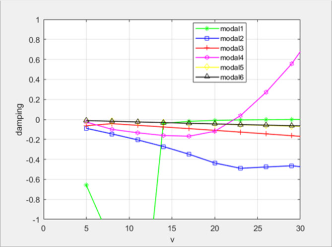
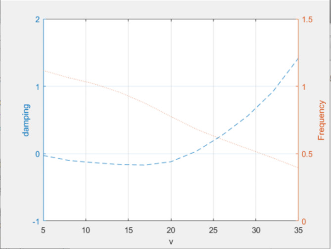
To carry out the flutter, the aerodynamic grid is established. The calculation of the aerodynamic force uses the dipole grid method, and the flutter calculation is performed using the p-k method. The aerodynamic model, spline and working condition settings are competed in Flightloads. The specific parameters are shown in Table 3. The speed range setting needs to be debugged many times, which is set to 5–35 m / s finally. The results are sent to Nastran for post-processing, and the first 6-order v-g diagram is shown in Fig. 2. Through the analysis of v-g diagram and vibration mode data, it can be seen that the flutter occurs in the third-order bending mode, and the frequency data of the third-order bending mode under the material are extracted as shown in Fig. 3.

Table 3.

Flutter condition parameters.

Parameters	Values
Atmospheric density	1.229 Kg/m3
Air-to-atmospheric density ratio	1
Mach number	0.1

Fig. 2.

v-g figure.

Fig. 3.

v-f figure.

Through flutter analysis, it is concluded that the flutter speed of 7050 aluminum wing is 22.3 m / s and the flutter frequency is 0.7 Hz. Wing flutter analysis of other materials is similar.

This paper applies MSC. Flightloads and MSC. Nastran 2018 for completing wing modeling and flutter analysis. Concretely, the flutter velocities of the wing are simulated by different metallic materials (7050 Aluminum alloy, 15-5PH stainless steel, Ti-6Al-4 V titanium alloy and 6061 aluminum alloy), different composite materials (T300/914, T300/1034-C, T300/976 and T300/5208), and different reduction ratios of the wing sizes (1:1.5, 1:1.7, 1:2, 1:3, 1:10 and 1:20) with 7050 Aluminum alloy materials are shown in Table 4.

Table 4.

Flutter velocity of high flexibility wings simulation.

Wing material	Velocity	Wing sizes reduction ratio (7050 aluminum alloy)	Velocity
7050 aluminum alloy	22.3	1:1.5	22.7
15-5PH stainless steel	37	1:1.7	21.83
Ti-6Al-4 V titanium alloy	27	1:2	20.27
6061 aluminum alloy	22	1:3	20.6
T300/914	20.2	1:10	22.35
T300/1034-C	19.8	1:20	26.79
T300/976	21.8
T300/5208	22.1

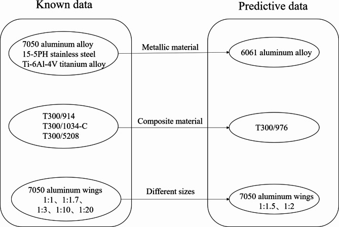
The data in Table 3 are separated into two groups, known flutter data and predicted flutter data, to confirm the accuracy of the trained NN’s prediction (see Fig. 4). The specific algorithm is as follows:

1. Metallic material: The flutter velocity of 7050 aluminum alloy, 15-5PH stainless steel, and Ti-6Al-4 V titanium alloy are used to train the NN to predict that of 6061 aluminum alloy.

2. Composite material: The flutter velocity of T300/914, T300/1034-C, and T300/5208 are used to train the NN to predict that of T300/976.

3. Wing Sizes: The flutter velocity of 7050 aluminum alloy with different sizes reduction ratios (1:1, 1:1.7, 1:3, 1:10, 1:20) are used to train the NN to predict that of other sizes reduction ratios (1:1.5, 1:2).

Fig. 4.

Classification of flutter data.

The architecture of neural networks

NN is a mathematical or computational model by duplicating the architecture and performance of the neural system in the brain of an individual²⁶. By strategically modifying the relationships between an immense number of nodes in the neural network, it mostly depends on the system’s complexity to accomplish the objective of information processing. NN is mainly used for function fitting and image recognition. It can continuously learn from the original data and find its characteristics to make predictions, which is very suitable for dealing with non-linear and complex data²⁷.

The structure of neurons

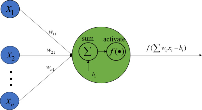
Throughout the training process, the weight term that represents the connections between all the different layers of neurons should be continually modified. A bias term is included in addition to the weight term for adjusting the neurons’ activity threshold. The activation function is used to add nonlinearity so as to enhance the NN’s capacity to match the input-output function. There are several common activation functions such as Sigmoid, ReLU, Tanh, etc. The structure of neurons is shown in Fig. 5.

Fig. 5.

Structure of neurons.

Structure and algorithm of back propagation neural network

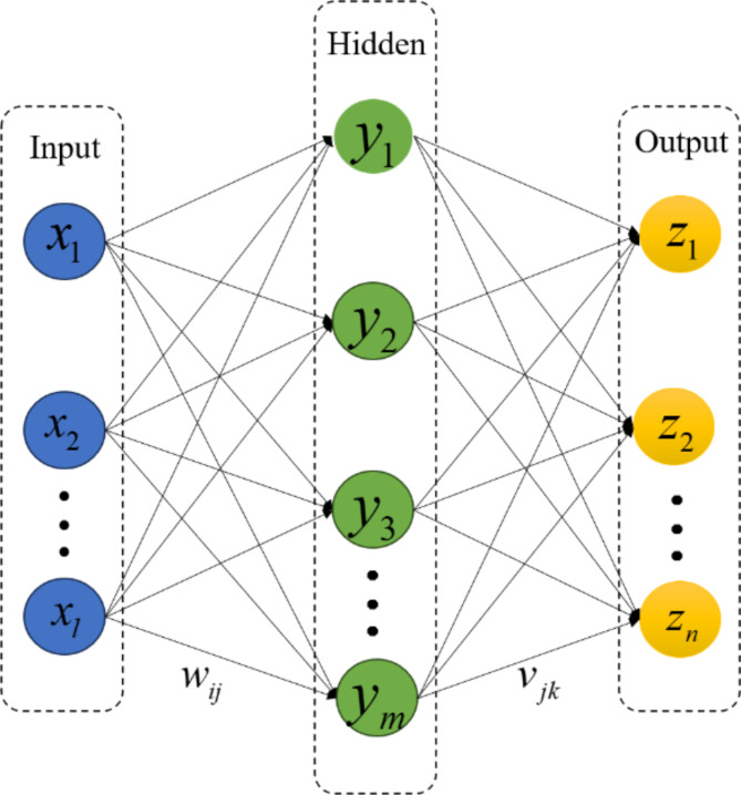
In this paper, an NN model trained using the error back propagation (BP) algorithm is utilized, called the BPNN. None of the neurons are connected to other neurons in the same layer, while they are fully connected to the neurons in previous layer. The weight term is rectified in reverse from the output layer until it returns to the input layer in the direction toward decreasing the expected output. Then the real output after the neurons in the output layer receive the input response of the network. The weight term can be continuously adjusted until the network output error is as small as possible^28,29. Three kinds of layers constitute the conventional BPNN: the input layer, the hidden layers, and the output layer, which are shown in Fig. 6.

Fig. 6.

The structure of NN.

It is assumed that there are neurons in each of the layers for input, hidden, and output. is the input of the neural network, while the outputs of the hidden layer and the output layer are and . is the expected output of the output layer. The weight items between the hidden layer and the output layer and the input layer are and , respectively. Furthermore, there are two bias terms: for the hidden layer and for the output layer.

The internal structure of the neuron can be employed to calculate the output values of the hidden layer and the output layer as follows.

4

5

where the activation function is represented by. The function employed in this research is the Sigmoid function.

The BPNN output and the expected output are used to compute the error , which is used to compute the loss by the Mean Square Error (MSE) .

6

7

The goal of neural network training is to minimize the loss function. Thus, optimization is usually required to update the NN parameters ().

Optimistic algorithm

BPNN uses the gradient descent algorithm³⁰ to adjust the parameters for network learning, which is the simplest to use and most easily understood. However, there are a few apparent drawbacks, including the longest time-consuming and lowest efficiency. Furthermore, the error function frequently has many minima considering the applied transfer function is a nonlinear function. Considering that the error first reaches the local minimum point, it is perhaps impossible to update the weight items and bias items to the global minimum point.

The Levernberg Marquardt (LM) algorithm^31,32 is implemented in this paper to update the NN’s parameters. Combining the gradient descent and Gauss-Newton methods, the LM algorithm enhances learning efficiency under guaranteeing quick convergence and avoiding the entire system from reaching the local minimum point.

Take the weight between the input layer and the hidden layer for example, the variables and are the both functions of . Similar to the Gauss-Newton method that expresses the Jacobi matrix of the first derivatives of the error function with respect to weights and thresholds as the Hessian matrix, the Hessian matrix of Jacobi matrix of can be expressed as:

8

The gradient can be expressed as Eq. (6).

9

The LM algorithm, similar to Newton’s method, corrects the weight items through an estimated Hessian matrix as follows.

10

All the parameters in the NN model can be corrected according to Eq. (7). Equation (7) becomes Newton’s method when the coefficient is 0, while it can be seen as the gradient descent approach with a smaller step size when the value of is high. In general, is initially given a tiny positive value, is progressively decreased by iteration, and is divided by a positive value that is greater than one. If a step cannot reduce the mean square error, is multiplied by and brought back to recalculate the weight item.

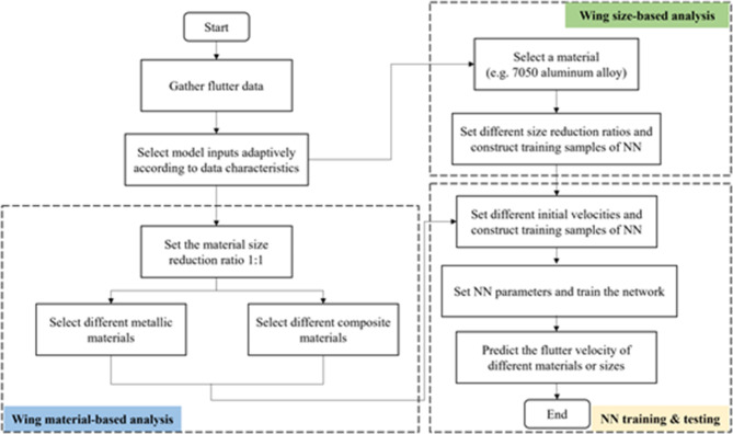
In the next two sections, we establish the framework of the neural network-based aeroelastic system identification for predicting flutter of high flexibility wings. Figure 7 shows the flowchart of the proposed method.

Fig. 7.

The flowchart of the NN approach for predicting flutter velocity.

NN training for high flexibility wings flutter

The design and implementation of NN

To train the high flexibility wings’ flutter data, it is essential to have a thorough understanding of the NN’s input and output variables. The main output variable is the wings’ flutter velocity. The input of the neural network in this paper includes the structural characteristics, flutter conditions, geometric dimensions and material properties of the wing.

This section demonstrates the simulation procedure of a BPNN based on the MATLAB neural network toolbox making use of the training process of 7050 aluminum alloy, 5-15PH stainless steel, and Ti-6Al-4 V titanium alloy data.

Given that the internal workings of the aeroelastic system that causes flutter are intricate, it is widely accepted that adding more hidden layers to a network can shorten training iterations and boost prediction accuracy. On the other hand, an excessive number of layers may result in overfitting and an extended training period. There is an identical issue with choosing the quantity of hidden layer nodes. It is the direct cause of overfitting during training and has a significant impact on the effectiveness of the well-established NN model. However, it cannot be ascertained in theory using a general and scientific procedure.

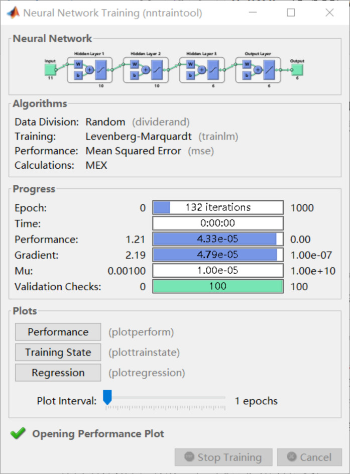
The present study employs the parameter debugging approach, i.e. the number of hidden layers and the number of neurons inside each layer are iterated continuously. Ultimately, a three-hidden-layer NN structure is established, with 10, 10, and 6 nodes in each layer, respectively. Other network training parameters are visualized by MATLAB’s integrated Neural Network Training toolbox, as shown in Fig. 8.

Fig. 8.

Neural network settings.

Figure 8 shows that the LM algorithm is employed as the training algorithm in this research. There are 132 training epochs. The highest MSE is computed to assess the network’s performance, which is less than 0.0433‰. This network has a gradient value of 0.0479‰.

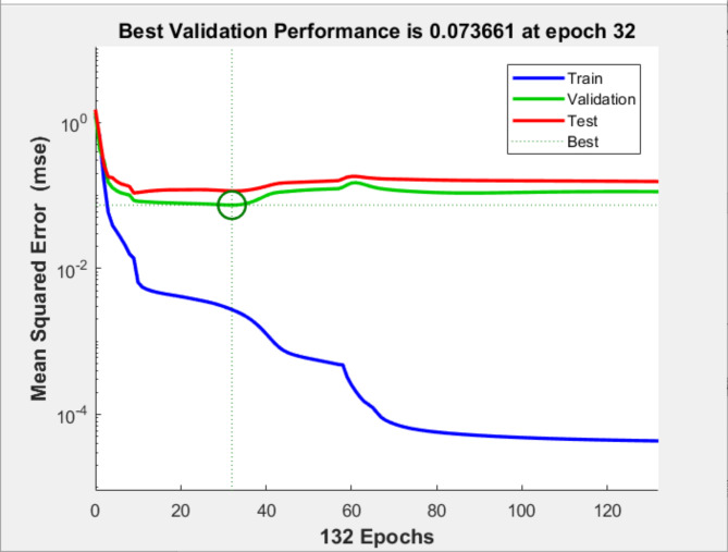
The plotperform function of MATLAB can be used to view the training of network performance. For example, Fig. 9 shows that the network reaches the minimum error at about 32 steps, and then over-fitting occurs, but the magnitude is not high, which will not significantly affect the prediction accuracy.

Fig. 9.

Mean square error curve.

High flexibility wings fitting for metallic materials

7050 aluminum alloy, 5-15PH stainless steel, and Ti-6Al-4 V titanium alloy data are used as sets of training data. Table 5 displays the specific parameters. Figure 10 shows the expected output, the predicted output and the error surface of the network.

Table 5.

Metallic material performance parameters.

	7050 aluminum alloy	5-15PH stainless steel	Ti-6Al-4 V titanium alloy
Elastic modulus	71	196.508	110.3
Density	2823	7833	4429
Poisson’s ratio	0.33	0.27	0.31

Fig. 10.

Fitting results of metallic materials.

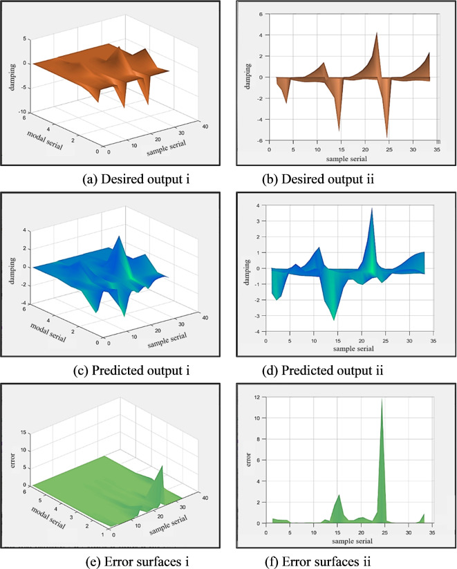
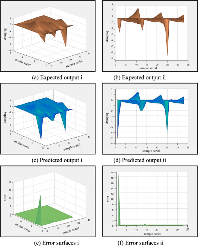
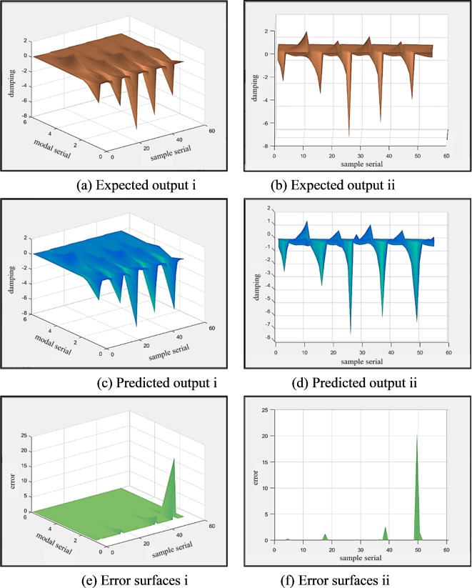
Each surface is defined by its x-, y-, and z-axes, which represent the sample serial number, modal serial number, and damping values, correspondingly. Figure 10(a)(c)(e) shows the trend of the damping values with modal serial and sample serial, while Fig. 10(b)(d)(f) are 2D view of the results with sample serial. It is the same in Figs. 11 and 12. Since the training data is the damping of 6 modes of 3 materials at 11 velocities, there are 33 samples, and each sample has 6 outputs, which are the damping of the first to sixth modes at the corresponding velocity.

Fig. 11.

Fitting results of composite materials.

Fig. 12.

Fitting results of different dimensions.

The samples are arranged according to velocity and material. Type I, II, and III are made of 7050 aluminum alloy, 5-15PH stainless steel, and Ti-6Al-4 V titanium alloy. The sample serials and their corresponding initial velocities are shown in Table 6.

Table 6.

The initial velocities of the sample serials.

Type	Sample serial	Material	Initial velocity	Velocity interval
I	1–11	7050 aluminum alloy	5–33 m/s	3 m/s
II	12–22	5-15PH stainless steel	20–60 m/s	4 m/s
III	23–33	Ti-6Al-4 V titanium alloy	15–45 m/s	3 m/s

To forecast flutter, one has to observe that whether the output surface’s z-axis is continually diverging and above the x-y plane. This will allow one to calculate the mode’s flutter. In essence, the error surface is maintained in the x-y plane. Because of the huge size, the first-order modal frequency is too low, resulting in a significant inaccuracy in the low-serial mode. First-serial modal damping diminishes with increasing velocity, but it quickly approaches 0-value damping. It is stable even if there is a gradual rising trend. The system starts to diverge after going to positive damping, but it is not flutter. Since it is currently a static aeroelastic problem, further study won’t be performed in this paper.

The network is more precise in dampening the development trend of the flutter mode, with the exception of the high error of the low-serial mode. As can be seen from Fig. 10, the mapping of input and output parameters is completed and the network essentially fits the modal damping at various velocities. It is apparent from the peak value analysis of the surface that the network effectively fits the flutter occurrence of 7050 aluminum alloy, 5-15PH stainless steel, and Ti-6Al-4 V titanium alloy under various modes. As a consequence, the BPNN effectively finishes the high-precision data fitting and identified the fluttering aeroelastic system.

High flexibility wings fitting for composite materials

In order to test the ability of BPNN to predict the flutter velocity of composite high flexibility wings, the input data of three kinds of graphite/epoxy resin composite fibers (T300/914, T300/1034-C and T300/5208) are used as training data. The performance parameters of the three composites are shown in Table 7. Given that the plate model serves as the foundation for wing modeling, composite materials should adhere to the traditional laminated plate theory, which states that strain perpendicular to the center surface is zero and that shear strain and shear stress perpendicular to the plate surface are ignored. Therefore, the composite material’s independent attribute parameters are restricted to the x-y direction. These four independent parameters include the plate surface’s Poisson’s ratio, the longitudinal elastic modulus, the transverse elastic modulus, and the shear modulus of the plate surface.

Table 7.

Composite material performance parameters.

Name / Properties of composite materials	T300/914	T300/1034-C	T300/5208
Longitudinal elasticity modulus	130	146.9	181
Transverse elastic modulus	4.65	11.4	10.3
Shear modulus	4.65	6.18	7.17
Density	1760	1800	1600
Poisson’s ratio	0.35	0.3	0.28

The inclusion of two parameters results in a significant decline in prediction ability when it comes to network configurations. There is a noticeable improvement when the number of concealed layers is increased, but the over-fitting becomes more apparent. After multiple trainings, there should be 10 concealed layers totally, with 6 nodes for the final layer and 13 nodes for the remaining layers.

The experimental data for T300/914, T300/1034-C, and T300/5208 are given in the number of 1 to 11 (Type I), 12 to 22 (Type II), and 23 to 33 (Type III). The initial velocities of them are listed in Table 8.

Table 8.

The initial velocities of the sample serials.

Type	Sample serial	Material	Initial velocity	velocity interval
I	1–11	T300/914	5–33 m/s	3 m/s
II	12–22	T300/1034-C	5–20 m/s	1.5 m/s
III	23–33	T300/1034-C	5-m/s	1.5 m/s

The specific fitting situation is shown in Fig. 11. Except for the first-order modal fitting of T300/914, the results demonstrate that the network fitting is good and other data does not show significant deviations.

High flexibility wings fitting for different sizes reduction ratios of the same material

Aiming at the high flexibility wings of 7050 aluminum alloy material when changing the size reduction ratios (1:1, 1:1.7, 1:3, 1:10 and 1:20) are used as training data. Debugging the network parameters results in the first hidden layer getting 11 nodes, but the other layers remain 10 and 6 nodes. With a total of 55 groups, the sample set is still set to 11 samples for the size of the wing flutter data, in the order of 1:1, 1:1.7, 1:3, 1:10, and 1:20. Table 9 shows the initial velocities of them.

Table 9.

The initial velocities of the sample serials.

Type	Sample serial	Wing size reduction ratio	Initial velocity	velocity interval
I	1–11	1:1	5–33 m/s	3 m/s
II	12–22	1:1.7	5–20 m/s	1.5 m/s
III	23–33	1:3	5–20 m/s	1.5 m/s
IV	34–44	1:10	5–20 m/s	1.5 m/s
V	45–55	1:20	5–20 m/s	1.5 m/s

Figure 12 illustrates how the network is fitted to the data. It is evident that even with a little amount of inaccuracy present in the 1:20 reduction ratio’s low-order modal damping, the network retains a high fitting accuracy even after the wing size is altered.

Predicting results of high flexibility wings’ flutter

High flexibility wings prediction for metallic materials

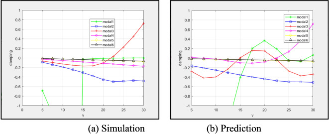
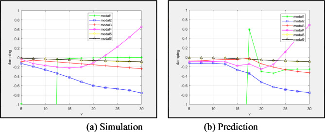
The network trained in Sect. "High flexibility wings fitting for metallic materials" is used to predict the flutter velocity of 6061 aluminum alloy high flexibility wings. Table 10 presents the material performance parameters. Figure 13 shows the results of 6061 aluminum alloy velocity-damping curve. Through a comparison of the simulation and prediction first 6-order modal velocity damping diagrams, it is shown that the network is unstable when forecasting the first and third modes, resulting in an early positive damping that eventually decays. The divergence induced by the first mode is also sooner than the simulation data. In addition, the initial flutter is the third mode, which becomes the fourth mode in the prediction, but the network’s expected flutter velocity is not considerably different. The simulation’s flutter velocity is 22, while the network predicting of the flutter velocity is 22.5.

Table 10.

6061 aluminum alloy performance parameters.

Parameters	Values
Elastic modulus	68.9
Density	2710
Poisson ratio	0.33

Fig. 13.

6061 aluminum alloy velocity-damping curve.

High flexibility wings prediction for composite materials

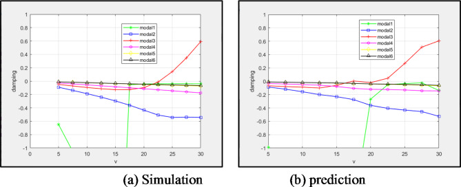
The network trained in Sect. 4.3 is implemented to estimate the flutter velocity of the T300/976 composite high flexibility wings. Table 11 provides the material performance parameters. Figure 14 shows the results of simulation and prediction for the first six orders of modal velocity-damping. It can be seen that the network exhibits an oscillation phenomenon when predicting the first mode. Nonetheless, the mode type is not affected. As the network predicts a flutter velocity of 23.9, compared to the model’s 21.8 in the simulation, it is obvious that the trained network can still forecast the aeroelastic system of the composite material’s high flexibility wings.

Table 11.

T300/976 performance parameters.

Parameters	Values
Longitudinal elasticity modulus	150
Transverse elastic modulus	9
Shear modulus	7.1
Density	1600
Poisson ratio	0.3

Fig. 14.

T300/976 velocity-damping curve.

High flexibility wings prediction for different sizes reduction ratios of the same material

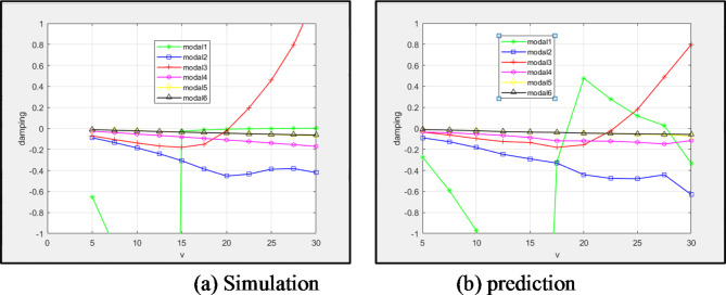
The network trained in Sect. 4.4 is implemented to estimate the flutter velocity with a reduction ratio of 1:1.5 and 1:2 (7050 aluminum alloy). The simulation and prediction results are displayed in Figs. 15 and 16. The first 6-order modal velocity damping diagram shows that the network trained with wing size changes is more adaptive to the 1:1.5 lessen model, each mode’s form is nearly precise, and the first mode in the 1:2 model does not fluctuate. The two models estimate flutter velocities of 16.5 and 22.05. Compared to the simulated flutter velocity, the 1:2 model’s flutter velocity prediction is more precise.

Fig. 15.

Wing size 1:1.5 velocity-damping curve (7050 aluminum alloy).

Fig. 16.

Wing size 1:2 velocity-damping curve (7050 aluminum alloy).

Conclusions

This paper proposes a system identification technique based on BPNN for predicting the flutter velocity of flexible wings. The multi-layer error of BPNN is trained by using the flutter data of the same size of different materials, as well as different sizes of the same material. The trained BPNN is used to predict the model with simulated flutter data, and the prediction ability of the BPNN to the unknown data is tested. The results show that the performance of the network is not good in the low-order mode, and the oscillation phenomenon often occurs, which confuses the occurrence of flutter and may cause incorrect mode of flutter. However, the accuracy of the predicted velocity is relatively high. Based on the identification results, the identification of the model by BPNN is reasonable and has certain credibility. The proposed NN-based method can solve the aeroelastic problem quickly and accurately in the preliminary design stage of the aircraft.

This method is particularly suitable for design tasks that need to evaluate the dynamic response of highly flexible wings, including large aircraft, drones and other application scenarios. The flexibility and weak parts of the wing are usually prone to flutter. In these cases, the traditional flutter analysis method may have a large amount of calculation, while the neural network can quickly provide more accurate prediction results by learning historical data.

Author contributions

Qing Guo: Conceptualization, methodology, formal analysis, investigation, writing—review & editing, project administration, resources.Xiaoqiang Li: Conceptualization, methodology, software, data curation, writing-original draft.Zhijie Zhou: Investigation, data curation, writing-original draft, software.Dexiao Ma: Formal analysis, resources, software.Yuzhuo Wang: Investigation, supervision, resources.

Data availability

The data presented in this study are available upon request from the corresponding authors. The data are not publicly available due to privacy.

Declarations

Competing interests

The authors declare no competing interests.

References

- 1.Dai, H. et al. A fast harmonic balance technique for periodic oscillations of an aeroelastic airfoil. J. Fluids Struct.50, 231–252 (2014). [Google Scholar]
- 2.Palaniappan, K. et al. Design of adjoint-based laws for wing flutter control. J. Aircr.48 (1), 331–335 (2011). [Google Scholar]
- 3.Chai, Y. et al. Aeroelastic analysis and flutter control of wings and panels: a review. Int. J. Mech. Syst. Dynamics. 1 (1), 5–34 (2021). [Google Scholar]
- 4.Mendes, P. V. M. & Gomes, G. F. Analysis of the influence of damage on flutter speed. CFRP Struct. Compos. Struct.280, 114931 (2022). [Google Scholar]
- 5.Fu, Z. & Liu, Z. Nonlinear flutter test of a very flexible wing. Lecture Notes Electr. Eng.459, 2627–2640 (2018). [Google Scholar]
- 6.Liu, F. et al. Calculation of wing flutter by a coupled fluid-structure method. J. Aircr.38 (2), 334–342 (2012). [Google Scholar]
- 7.Huang, R. et al. Design of active flutter suppression and wind-tunnel tests of a wing model involving a control delay. J. Fluids Struct.55, 409–427 (2015). [Google Scholar]
- 8.Warwick, G. EU researchers actively suppress flutter in flight tests. Aerosp. Dly. De?F. Rep.24, 285 (2023). [Google Scholar]
- 9.Dimitriadis, G. & Cooper, J. E. Flutter prediction from flight flutter test data. J. Aircr.38 (2), 355–367 (2012). [Google Scholar]
- 10.Zhang, W. et al. A flutter prediction method with low cost and low risk from test data. Aerosp. Sci. Technol.86, 542–557 (2019). [Google Scholar]
- 11.Sudha, U. P. V., Deodhare, G. S. & Venkatraman, K. A comparative assessment of flutter prediction techniques. Aeronaut. J.124 (1282), 1945–1978 (2020). [Google Scholar]
- 12.Georghiades, G. A. & Banerjee, J. R. Flutter prediction for composite wings using parametric studies. AIAA J.35 (4), 756–748 (2012). [Google Scholar]
- 13.Mohammadi-Amin, M. & Ghadiri, B. An aeroelastic metamodel based on experimental fata for flutter prediction of swept rectangular wings. J. Appl. Fluid Mech.6 (1), 115–120 (2013). [Google Scholar]
- 14.Mayuresh, J. P. & Dewey, H. H. Flight dynamics of highly flexible flying wings. J. Aircr.43 (6), 1790–1798 (2006). [Google Scholar]
- 15.Fernández, F., Cleaver, D. & Gursul, I. Unsteady aerodynamics of flexible wings in transverse gusts. J. Fluids Struct.108, 103425 (2022). [Google Scholar]
- 16.Fu, Z. et al. Experimental study on structural dynamic characteristics of flexible high-aspect-ratio wings. Acta Aeronautica Et Astronaut. Sinica. 34 (9), 2177–2184 (2013). [Google Scholar]
- 17.Huang, R. et al. Nonlinear reduced-order models for transonic aeroelastic and aeroservoelastic problems. AIAA J.56 (9), 3718–3721 (2018). [Google Scholar]
- 18.Yao, X. et al. Transonic aerodynamic–structural coupling characteristics predicted by nonlinear data-driven modeling approach. AIAA J.62 (3), 1159–1178 (2024). [Google Scholar]
- 19.Huang, R., Hu, H. & Zhao, Y. Nonlinear reduced-order modeling for multiple-input/multiple-output aerodynamic systems. AIAA J.52 (6), 1219–1231 (2014). [Google Scholar]
- 20.Savaresi, S. M., Bittanti, S. & Montiglio, M. Identification of semi-physical and black-box non-linear models: the case of MR-dampers for vehicles control. Automatica41 (1), 113–127 (2005). [Google Scholar]
- 21.Scott, R. C. & Lawrence, E. P. Active control of wind-tunnel model aeroelastic response using neural networks. J. Guidance Control Dynamics. 23 (6), 1100–1108 (2000). [Google Scholar]
- 22.Mattaboni, M., Quaranta, G. & Mantegazza, P. Active flutter suppression for a three-surface transport aircraft by recurrent neural networks. J. Guidance Control Dynamics. 32 (4), 1295–1307 (2012). [Google Scholar]
- 23.Pitt, D. M., Haudrich, D. P. & Conference Determination of the flutter critical stores configuration utilizing an optimized artificial neural network. AIAA 2007–2365. 48th AIAA/ASME/ASCE/AHS/ASC Structures, Structural Dynamics, and Materials April. (2007).
- 24.Wu, Y. & Feng, J. development and application of artificial neural network. Wireless Personal Communications, 102: 1645–1656. (2018).
- 25.Mu, X. et al. Machine learning-based active flutter suppression for a flexible flying-wing aircraft. J. Sound Vib.529 (7), 116916 (2022). [Google Scholar]
- 26.Basheer, I. A. & Hajmeer, M. Artificial neural networks: fundamentals, computing, design, and application. J. Microbiol. Methods. 43 (1), 3–31 (2000). [DOI] [PubMed] [Google Scholar]
- 27.Ugalde, H. M. R. et al. Computational cost improvement of neural network models in black box nonlinear system identification. Neurocomputing166 (20), 96–108 (2015). [Google Scholar]
- 28.Li, X. et al. Establishing a dynamic self-adaptation learning algorithm of the bp neural network and its applications. Int. J. Bifurcat. Chaos. 25 (14), 1540030 (2015). [Google Scholar]
- 29.Chen, J. & Chen, Q. Application of deep learning and bp neural network sorting algorithm in financial news network communication. J. Intell. Fuzzy Syst.38 (6), 7179–7190 (2020). [Google Scholar]
- 30.Wang, M., Wang, N. & Li, X. Improvement and application of BPNN algorithm. Comput. Eng. Appl.45 (35), 47–48 (2009). [Google Scholar]
- 31.Hashemi, S. M., Rezapour, M. & Moradi, A. An effective hybrid PSO-based algorithm for planning UMTS terrestrial access networks. Eng. Optim.42 (3), 241–251 (2010). [Google Scholar]
- 32.Kallapur, A. G. et al. Nonlinear estimation of ring-down time for a fabry-perot optical cavity. Opt. Express. 19 (7), 6377–6386 (2011). [DOI] [PubMed] [Google Scholar]
Associated Data
This section collects any data citations, data availability statements, or supplementary materials included in this article.
Data Availability Statement