Abstract
Accurately estimating forest carbon sink and exploring their climate-driven mechanisms are critical to achieving carbon neutrality and sustainable development. Fewer studies have used machine learning-based dynamic models to estimate forest carbon sink. The climate-driven mechanisms in Shangri-La have yet to be explored. In this study, a genetic algorithm (GA) was used to optimize the parameters of random forest (RF) to establish dynamic models to estimate the carbon sink intensity (CSI) of Pinus densata in Shangri-La and analyze the combined effects of multi-climatic factors on CSI. We found that (1) GA can effectively improve the estimation accuracy of RF, the R2 can be improved by up to 34.8%, and the optimal GA-RF model R2 is 0.83. (2) The CSI of Pinus densata in Shangri-La was 0.45–0.72 t C·hm− 2 from 1987 to 2017. (3) Precipitation has the most significant effect on CSI. The combined weak drive of precipitation, temperature, and surface solar radiation on CSI was the most dominant drive for Pinus densata CSI. These results indicate that dynamic models can be used for large-scale long-term estimation of carbon sink in highland forest, providing a feasible method. Clarifying the driving mechanism will provide a scientific basis for forest resource management.
Keywords: Forest aboveground carbon sink, Time series, Dynamic modeling, Genetic algorithm, Climate change
Subject terms: Carbon cycle, Climate-change impacts, Forestry
Introduction
As a major component of terrestrial ecosystem, forest possesses significant carbon sink potential1. Forest carbon sink (CS) refers to the process by which green plants absorb CO2 from the atmosphere through photosynthesis and sequester it within the forest, playing a crucial role in global climate change mitigation2. Forest carbon sink accounts for 76–98% of terrestrial carbon sink, holding an important position in the global carbon sink landscape3,4. In recent years, forest carbon sink have garnered widespread attention due to their substantial economic and ecological value, becoming a vital strategy for addressing climate change and achieving carbon neutrality5. Effective monitoring and assessment of forest carbon sink capacity are essential for maintaining the carbon balance of terrestrial ecosystems, achieving efficient management of forest resources, and mitigating climate warming6.
The estimation of forest carbon sink can be achieved through quantitative analysis of variations in forest carbon stock over specific periods7. Remote sensing-based estimation is one of the best methods for large-scale and long-term studies8. Because of their long lifetime and good data continuity, Landsat satellites are an ideal data source for time series studies9. Machine learning algorithms are important tools for estimating CS based on remote sensing images, and they are widely used in assessing forest resources such as aboveground biomass (AGB) and carbon stock10. Models established by the Random Forest (RF) method demonstrate higher stability and accuracy11,12, effectively avoiding the underestimation of CS seen in some ecosystem process models13. Zeng et al.13 compared the performance of the RF, CASA, and GLOPEM model in estimating NEP on the Tibetan Plateau. They found that the RF model had the highest estimation accuracy in the plateau region. Liao et al.14 used several machine learning algorithms to establish models to estimate aboveground carbon stock (AGCS) of Pinus densata in Shangri-La, and the results showed that the estimation model established by RF fitted the best. Although RF has been proven to be a mature machine learning algorithm, its parameter tuning is still an unstable process15 and is under-explored for parameter optimization. Genetic Algorithm (GA) is a commonly used optimization algorithm. GA can further improve the machine learning model accuracy and increase stability by adjusting multiple model parameters16. We use genetic algorithms to optimize the random forest algorithm to explore the model construction problem in depth so as to provide both model optimization ideas and new methods for forest carbon sink estimation.
The dynamic model is a process-based model with strong data correlation over a long time series17. Zhang et al.18 established steady-static and dynamic models, respectively, and found that the dynamic model has higher accuracy in forest AGB estimation. Gómez et al.19 established models by dividing the change process into state variables (steady-state) and process variables (dynamic), and the results showed that the process variable model is more predictive than the state variable model in forest AGB. Meanwhile, the dynamic model allows for evaluating time-dependent phenomena and the period needed for recovery19. While steady-state models remain the foundation for forest resource estimation, dynamic models provide researchers with new perspectives. Currently, studies applying dynamic models to forest carbon sink estimation are relatively rare, making this attempt highly valuable. Since forest carbon sink is a dynamic variable, we established a dynamic model based on this theory to analyze the long-term changes in forest carbon sink accurately.
Global warming has become an undeniable fact, and with the intensification of climate change, the capacity of terrestrial CS will be significantly affected20. Forest carbon sink is particularly sensitive to climate change and is more significantly affected by it21. Hubau et al.22 assessed the carbon sink capacity of tropical African and Amazonian forests and found that increasing temperatures reduced the carbon sink capacity of both forests. Xu et al.23 used the structural equation model to analyze the drivers of forest AGB in Shangri-La, and the results showed that climatic factors significantly influenced forest AGB but did not indicate the specific roles of each factor. Previous analyses of the climatic drivers of AGB or AGCS of forest in Shangri-La only considered the degree of influence. They did not take into account the interactions between factors, such as synergistic and antagonistic effects. The climate-driving mechanism of the CS in Pinus densata needs to be determined. Therefore, we used partial correlation analysis to eliminate the effects of uncorrelated factors. The multi-correlation analysis was then used to quantify climatic factors’ spatial and temporal impacts of on forest carbon sink by considering the interactions among multiple factors.
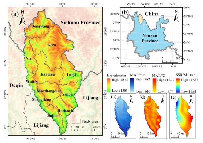
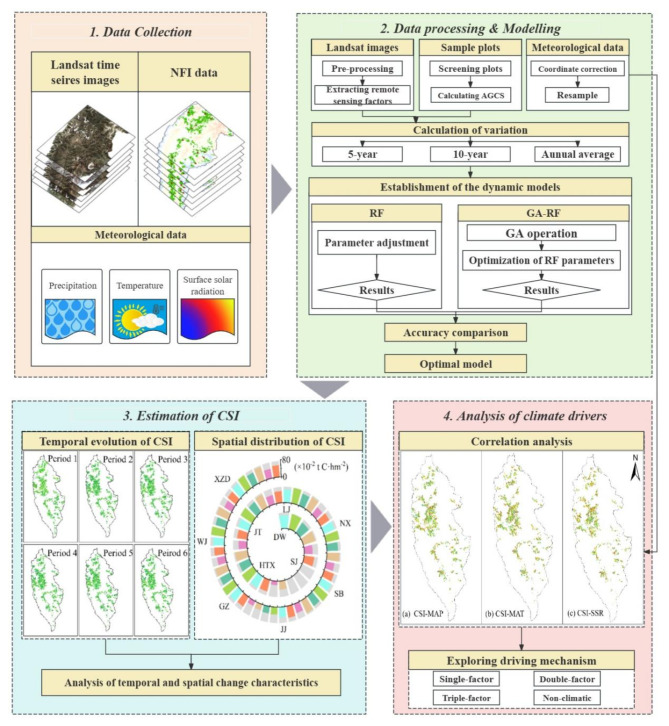
Shangri-La is a typical ecological carbon sink in China’s Yunnan Province, and its geomorphologic and climatic characteristics highly represent of southwestern China (Fig. 1). Pinus densata is one of the dominant tree species in Shangri-La. In addition to Yunnan, Pinus densata is also widely distributed in Sichuan and Tibet and plays an important role in the carbon cycle in southwest China. Shangri-la is located southwest of the Qinghai-Tibet Plateau, with complex terrain, a changeable climate, and a fragile ecological environment, so it is challenging to accurately estimate forest carbon sink intensity (CSI). Besides, the climate-driving mechanism of the CSI of Pinus densata is still unclear. Therefore, in this study, remote sensing-based dynamic models were used to estimate the carbon sink capacity of Pinus densata in Shangri-La, and correlation analysis methods were used to explore the climate driving mechanism (Fig. 2). The main objectives are the following: (1) establishing carbon sink dynamic models based on three different types of variation; (2) analyzing the effect of GA on RF dynamic models; (3) estimating the carbon sink of Pinus densata in Shangri-La and analyze its temporal and spatial changes; (4) exploring the climate driving mechanism.
Fig. 1.
Location and climate information map of the study area. (a) overview of Shangri-La’s administrative divisions; (b) Shangri-La location overview map in Yunnan province, China; (c), (d) and (e) map of total meteorological averages value from 1987–2017: mean annual precipitation (MAP), mean annual temperature (MAT), and (e) mean annual surface solar radiation (SSR). The DEM data in (a) were obtained from https://www.gscloud.cn/. MAP, MAT and SSR data in (c), (d), (e) were obtained from https://data.tpdc.ac.cn/. All data were resampled, cropped and spliced using ArcGIS 10.8 (https://www.arcgis.com/).
Fig. 2.
Workflow of the study. (DW: Dongwang; GZ: Geza; HTX: Hutiaoxia; JT: Jiantang; LJ: Luoji; NX: Nixi; SB: Sanba; XZD: Xiaozhongdian; SJ: Shangjiang; JJ: Jinjiang; WJ: Wujing. The same as below.)
Results
Analysis of modeling
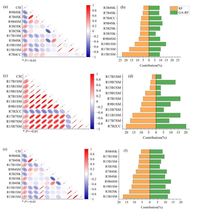
For each of the three types of variation, we selected 10 of the most substantial correlated remote sensing factors, all of which exhibited highly significant correlations (P < 0.01) suitable for modeling (Table 1; Fig. 3). The optimal modeling factors with strong and highly significant correlations among the three types of variation were all texture feature factors, among which SK and SM appeared most frequently.
Table 1.
Screening factor for each type of variation. Where the naming form of the texture factor is RXBYFF, where R is the texture window, X is the size of the window, and the value of X is an odd number within 1 ~ 19 (including 1 and 19); BY is a specific single band of the image, and the value of Y is 1 ~ 5 and 7; FF is the abbreviation of texture factor. For example, R9B4SK is the SK of the fourth band under the 9 × 9 window.
| Variation type | Remote sensing factors |
|---|---|
| 5-year variation |
R9B4SK, R7B4SK, R9B4SM, R3B3SK, R3B2SK, R17B1SM, R3B4SK, R19B1SM, R15B1SM, R7B4CC |
| 10-year variation |
R11B1SM, R7B1SM, R9B1SM, R15B7SM, R17B7SM, R17B1SM, R19B7SM, R19B1SM, R15B1SM, R7B2CC |
| Annual average variation |
R9B4SK, R7B4SK, R9B4SM, R3B3SK, R3B2SK, R17B1SM, R3B4SK, R19B1SM, R15B1SM, R13B1SM |
Fig. 3.
The correlation and contribution degree of each model’s modeling factors. (a) and (b), top 10 factors in the 5-year variation; (c) and (d), top 10 factors in the 10-year variation; (e) and (f), top 10 factors in the Annual average variation. (a), (c) and (e), Pearson’s correlation analysis results. (b), (d) and (f), the contributions of modeling factors.
Table 2 shows the optimal parameters of each RF model established by the three variations. Table 3 shows the optimal parameters of the GA-RF models, which were optimized to spend exponentially more time on training than RF models. In addition, all six dynamic models ranked the input factors by their importance and output the modeling contribution values of each factor (Fig. 4).
Table 2.
Optimum parameters of RF
| Variation type | n_estimators | max_depth | min_samples_leaf | min_samples_split |
|---|---|---|---|---|
| 5-year variation | 90 | 10 | 1 | 1 |
| 10-year variation | 40 | 10 | 2 | 1 |
| Annual average variation | 170 | 10 | 1 | 1 |
Table 3.
Optimum parameters of GA-RF.
| Variation type | n_estimators | max_depth | min_samples_leaf | min_samples_split |
|---|---|---|---|---|
| 5-year variation | 80 | 20 | 2 | 1 |
| 10-year variation | 60 | 20 | 2 | 1 |
| Annual average variation | 70 | 10 | 2 | 1 |
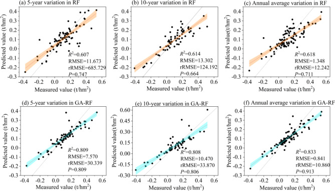
The accuracy of the six dynamic models is shown in Fig. 4. Among the dynamic models with each type of variation, the R2 and P of the GA-RF model are greater than that of the RF model, and the RMSE is smaller than that of the RF. Combining the evaluation metrics, the GA-RF fit based on the annual average variation is the best. This fit improved the R2, lowered the RMSE, and improved the P compared with the optimal conventional RF model. This result shows that the accuracy of the RF-based dynamic model is improved after GA optimization.
Fig. 4.
Comparison of dynamic modeling results.
As shown in Fig. 6, R2, rRMSE, and P of the GA-RF model based on annual mean change are better than that of other types of the GA-RF models. Due to the different time scales, the RMSE should be standardized to the same scale when making comparisons14. After multiplying the RMSE of the 5-year variation by 2 and the annual average variation by 10, we found that GA-RF based on the annual average change possesses the smallest RMSE. Thus, the GA-RF model accuracy of the annual average variation is better than that of the models with the 5-year and 10-year variation, which is the optimal dynamic model.
Fig. 6.
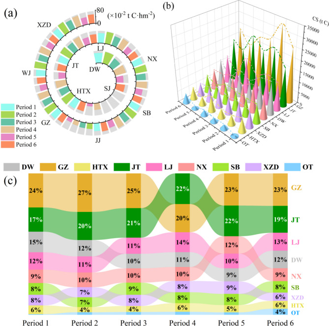
CSI and CS in Shangri-La townships in all periods, 1987–2017. (a) CSI by township from 1987 to 2017; (b) CS by township from 1987 to 2017; (c) percentage of CS by township in each period. OT: Other townships. Here, OT refers to the sum of the CS of the Sanjiang, Jinjiang and, Wujing.
Estimation of CSI
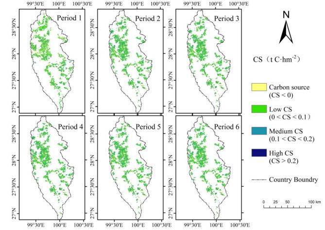
From 1987 to 2017, we divided the period into six intervals of five years each. According to the model evaluation results, the GA-RF model based on annual average variation was used to estimate CS. By integrating the area on Pinus densata distribution, we derived the spatial distribution map of total CS of Pinus densata in Shangri-La (Fig. 5). The total CS for periods 1–6, respectively, were 10.53 × 10⁴ t C, 12.35 × 10⁴ t C, 10.17 × 10⁴ t C, 11.75 × 10⁴ t C, 7.84 × 10⁴ t C and 10.2 × 10⁴ t C. The CSIs for periods 1–6, respectively, were 0.61 t C·hm− 2, 0.72 t C·hm− 2, 0.6 t C·hm− 2, 0.67 t C·hm− 2, 0.45 t C·hm− 2, 0.55 t C·hm− 2.
Fig. 5.
Shangri-La’s CS by periods (Period 1 is 1987–1992, Period 2 is 1992–1997, Period 3 is 1997–2002, Period 4 is 2002–2007, Period 5 is 2007–2012 and Period 6 is 2012–2017).
From 1987 to 2017, the CSI of Pinus densata in Shangri-La fluctuated between 0.45 and 0.72 t C·hm− 2. There was a general declining trend, decreasing from 0.61 t C·hm− 2 in Period 1 to 0.55 t C·hm− 2 in Period 6. The period with the most potent carbon sink capacity was Period 2, with a CSI of 0.72 t C·hm− 2, while the weakest period was Period 5, with a CSI of 0.45 t C·hm− 2. However, compared to the end of the last century, the overall CSI of Pinus densata in Shangri-La has tended to stabilize, showing slight variation.
From 1987 to 2017, The average CSI for Shangri-La from 1987 to 2017 was 60.14 × 10− 2 t C·hm− 2. Most townships demonstrated a strong carbon sink capacity, although the distribution of Pinus densata area varied among townships (Fig. 6a). The average CSIs of Xiaozhongdian, Hutiaoxia, Sanba, Geza, and Luoji were 60.29 × 10− 2 t C·hm− 2, 60.26 × 10− 2 t C·hm− 2, 60.20 × 10− 2 t C·hm− 2, 60.19 × 10− 2 t C·hm− 2, and 60.15 × 10− 2 t C·hm− 2, respectively, which are higher than the average CSI of Shangri-La. These five townships are therefore high CSI areas. The average CSIs of Jiantang, Wujing, Dongwang, and Nixi were 60.13 × 10− 2 t C·hm− 2, 60.12 × 10− 2 t C·hm− 2, 60.11 × 10− 2 t C·hm− 2, and 60.06 × 10− 2 t C·hm− 2, respectively, which were slightly lower than the average CSI of Shangri-La. These four townships are therefore medium CSI areas. The average CSIs of Shangjiang and Jinjiang were 19.30 × 10− 2 t C·hm− 2 and 37.38 × 10− 2 t C·hm− 2, respectively, which were significantly lower than the average CSI of Shangri-La, making them low CSI areas.
In terms of total CS values, there was a large disparity between townships (Fig. 6b). The CS of Geza and Jiantang accounted for a high proportion of total CS in Shangri-La all year round, both exceeding 15%. These two townships had a strong carbon sink capacity and make important contributions to Shangri-La’s sink. The CS of Luoji, Dongwang and Nixi accounted for between 9% and 15% of total CS of Shangri-La and had a high carbon sink capacity. Although Xiaozhongdian, Hutiaoxia and Sanba had high CSI, these three townships had low CS values. The remaining townships had a very low CS share and poor carbon sink capacity (Fig. 6c). However, Shangri-La maintained a stable carbon sink capacity from 1987 to 2017 due to positive CS values in all townships.
Analysis of climate driving force
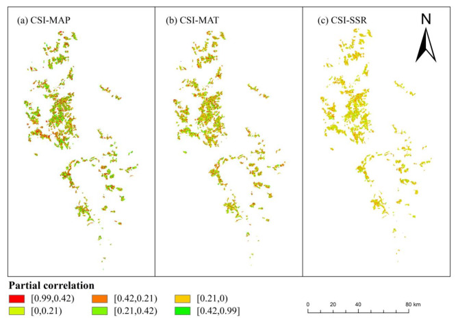
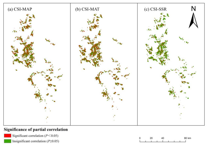
Pixel level analysis of the correlation of CSI of Pinus densata with MAP, MAT, and SSR temporal changes from 1987 to 2017 based on the partial correlation coefficient and T-test (Figs. 7 and 8). The mean value of the partial correlation coefficient between MAP and CSI was 0.018. The area with a positive correlation accounted for 51.41% of the total area. The positively correlated areas accounted for 35.65% of the area and were distributed throughout Shangri-La, mainly in the central region. The negatively correlated areas accounted for 48.59% of the total area, and the significantly negatively correlated areas accounted for 32.84% of the total area, distributed in the southern part of the study area with low CSI.
Fig. 7.
Partial correlation between CSI and climatic factors. (a) CSI and MAP; (b) CSI and MAT; (c) CSI and SSR.
Fig. 8.
Significance of partial correlation between CSI and climatic factors. (a) CSI and MAP; (b) CSI and MAT; (c) CSI and SSR.
The mean value of the partial correlation coefficient between MAT and CSI was − 0.015, with 48.24% of the area positively correlated and 32.62% significantly positively correlated. The proportion of negatively correlated areas was 51.76%, and the proportion of significantly negatively correlated areas was 36.31%. Both positively and negatively correlated areas were distributed throughout the whole territory, without being concentrated in a particular region.
The mean value of the partial correlation coefficient between SSR and CSI was − 0.013. The positive correlation areas accounted for 45.09% of the total area, of which the significant positive correlation areas accounted for 24.77%, mainly in the central part of the study area. The area of negatively correlated areas accounted for 54.91%, of which 31.75% were significantly negatively correlated, mainly in the northern part of the study area.
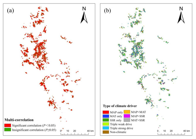
The mean multi-correlation coefficient between CSI and climate factors in Shangri-La is 0.65 (P < 0.05), showing that the comprehensive impact of climate change significantly promotes the growth of CSI of Pinus densata in this area. There are no notable spatial differences in the overall correlation between CSI and climatic factors. Regions with highly significant positive correlations account for 35.36% of the total area of the study region and are widely distributed throughout the area (Fig. 9).
Fig. 9.
Multi-correlation between CSI and climate factors and climate-driven mechanisms of Pinus densata in Shangri-La. (a) Multi-correlation between CSI and climatic factors; (b) climate-driven types of zoning in CSI and their area share.
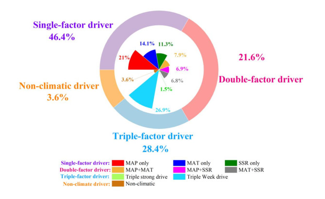
In Shangri-La, 96.42% of the variation in CSI of Pinus densata is driven by climatic factors (Fig. 10). Among these, the areas jointly influenced by MAP, MAT, and SSR account for the most significant proportion, reaching 26.91%, and are widely distributed throughout the study area. In the single-factor driver, the proportion of areas driven by MAP only is 21%, significantly higher than those influenced by MAT and SSR. Specifically, areas driven by MAP only are primarily located in the northern and northeastern Shangri-La; areas driven by MAT only are mainly concentrated in the central, while areas influenced by SSR only are distributed across the central and southern Shangri-La. The areas influenced by other types of climatic drivers on CSI account for less than 10% and are dispersed within the study area.
Fig. 10.
Area share of climate-driven mechanism types for CSI change in Pinus densata.
In summary, it is evident that MAP has the most significant impact on CSI among all driving factors, whether acting independently or in conjunction with others. This result indicates that precipitation is the primary driving factor affecting the CSI of Pinus densata. Furthermore, the area influenced by multiple factors exceeds that influenced by single factors, suggesting that climate factors primarily exert their effects on the CSI of Pinus densata through synergistic interactions.
Discussion
The advantage of time series images is that they can reduce the influence of uncertainty factors in modeling single-period data and improve the accuracy and reliability of modeling24. It is also an important basis for establishing dynamic models. Relying on the NFI and Landsat time-series images accumulated over 30 years, we can calculate the changes in AGCS and remote sensing factors and thus establish dynamic models. In recent studies on machine learning models for estimating forest carbon fluxes13,25,26, the R2 of machine learning-based steady-state models ranged from 0.42 to 0.72. In contrast, the optimal model in this study has an R2 of 0.83, which is significantly more accurate. This result suggests that dynamic modeling can be a better choice for high accuracy and low error in forest resource estimation, especially in time series studies, and provide a new idea for CS estimation.
Model parameters are adjustable values that impact the training of the model and its performance15, which in turn can affect the model’s stability and accuracy27. In this study, four important parameters of RF were selected for optimization. These parameters were manually adjusted before modeling to establish the best-fitting three RF dynamic models. Subsequently, we used GA for parameter optimization and established GA-RF dynamic models based on three types of variation. All of their accuracy evaluation indexes were significantly improved, indicating the improved performance and fitting of the GA-RF dynamic model. Machine learning models have been applied to estimate carbon fluxes in ecosystems such as grasslands28 and agricultural fields29. Therefore, the results of this study may provide new ideas for optimizing carbon sink estimation models for other ecosystems.
Currently, there are fewer studies on CS estimation of Pinus densata in Shangri-La, so we refer to some scholars14,24,30,31 for the research results on AGB and AGCS of Pinus densata in Shangri-La City from 1987 to 2017. Table 4 shows a significant difference between the CSI obtained by directly estimating and the CSI obtained by estimating the AGCS and then calculating the change. In terms of estimated values, the results of this study are similar to those of Han et al.30. Regarding the trend of change, the results of this study are similar to Liao et al.14 and Teng et al.24. Pinus densata in Shangri-La showed a carbon sink from 1987 to 2017. This result consistent with Yin et al.31.
Table 4.
Different researchers’ results of changes of AGCS and CSI estimation of Pinus densata in Shangri-La.
| Year |
 AGCS (×104 t C) AGCS (×104 t C) |
CSI (t C·hm− 2) | Source | Methodology |
|---|---|---|---|---|
| 1987–1992 | -53.33 | -3.11 | Liao et al.14 | RF model with the addition of topographic factors |
| 1992–1997 | 13.89 | 0.81 | ||
| 1997–2002 | -94.04 | -5.51 | ||
| 2002–2007 | 14.60 | 0.84 | ||
| 2007–2012 | 20.87 | 1.20 | ||
| 2012–2017 | 5.62 | 0.30 | ||
| 1987–1992 | -40.52 | 2.36 | Teng et al.24 | RF model |
| 1992–1997 | 150.00 | 8.74 | ||
| 1997–2002 | -62.20 | -3.65 | ||
| 2002–2007 | -7.96 | -0.46 | ||
| 2007–2012 | 15.64 | 0.90 | ||
| 2012–2017 | 153.36 | 8.35 | ||
| 1987–1992 | -83.97 | -3.82 | Han et al.30 | Nonlinear mixed-effects model |
| 1992–1997 | 0.19 | 0.01 | ||
| 1997–2002 | 31.37 | 1.84 | ||
| 2002–2007 | 3.50 | -0.20 | ||
| 2007–2012 | 21.48 | 1.23 | ||
| 2012–2017 | 65.04 | 3.52 | ||
| 1987–1992 | 125.17 | 7.30 | Yin et al.31 | RF model with the addition of climatic factors |
| 1992–1997 | 62.13 | 3.64 | ||
| 1997–2002 | 47.81 | 2.69 | ||
| 2002–2007 | -54.97 | 3.16 | ||
| 2007–2012 | 72.90 | 4.18 | ||
| 2012–2017 | 398.23 | 21.55 | ||
| 1987–1992 | 10.53 | 0.61 | This study | GA-RF dynamic model |
| 1992–1997 | 12.35 | 0.72 | ||
| 1997–2002 | 10.17 | 0.60 | ||
| 2002–2007 | 11.75 | 0.67 | ||
| 2007–2012 | 7.84 | 0.45 | ||
| 2012–2017 | 10.20 | 0.55 |
By conducting single-factor and combined multifactor correlation analyses of climatic factors on the CSI of Pinus densata, we found that precipitation showed a positive effect on the CSI of Pinus densata, and temperature and surface solar radiation showed an inverse effect on the CSI of Pinus densata. Global warming and the increased frequency of droughts, which restrict Pinus densata growth32, has made Pinus densata very sensitive to changes in temperature. Thus, an increase in air temperature inhibits the growth of Pinus densata, while an increase in precipitation relieves the moisture limitation that limits its growth process. The effects of climatic factors on CS often do not act alone but are coupled by multiple factors33,34. A combination of climatic factors contributed to the growth of the CSI of Pinus densata in Shangri-La during the study period, and the CSI of Pinus densata was mainly weakly driven by MAP, MAT, and SSR. This result is similar to that of Xu et al.33 in southwest China.
Although the CSI of Pinus densata in Shangri-La increased between 1992 and 1997, the total CS was not significantly elevated due to the decrease in Pinus densata area due to land use change30. The CSI of Pinus densata declined during 1997–2002. This phenomenon was caused by irregular logging behavior and more dry weather in Shangri-La during this period23. Since 2000, the Natural Forest Protection Project and the Returning Cultivated Land to Forestry Project began to be implemented35. Yunnan Province’s forest resources have been protected, and the CSI has been steadily improved. Yunnan Province experienced severe drought impacts from 2007 to 2012, especially the historic drought in Yunnan Province in 201036. Therefore, extreme drought can greatly reduce the CSI of Pinus densata. After 2012, with improved climatic conditions and adherence to previous policies, Pinus densata area increased, so both CSI and total CS values increased. Research suggests that future climatic conditions on the plateau may tend towards a “wet and warm” climate with high precipitation and increased temperatures6. Under these climatic conditions, Pinus densata in Shangri-La has a substantial carbon sink capacity. In the future, Pinus densata will continue to play an important role in carbon emission reduction and carbon sequestration in northwestern Yunnan.
In this study, we propose a method to estimate aboveground CS in forest based on long time series and quantify the effects of climate factors on forest CS at the pixel level. Compared to previous studies, this study has several methodological highlights. Firstly, We used dynamic models with good compatibility with time-series images to directly estimate forest carbon sink using the amount of change as the modeling basis. Secondly, this study used GA to optimize the parameters of the RF dynamic model, and the GA-RF model is more stable and accurate than the RF model. Finally, previous climate-driven studies in the Shangri-La mainly focused on the degree of influence of single factors. We consider the role of single factors and combined multifactors on the CSI of Pinus densata separately to explore the climate-driven mechanisms in Shangri-La. However, this study has limitations and potential areas for future improvement. Firstly, due to data limitations, this study only estimated CS in the aboveground portion of the forest and did not estimate CS in the belowground portions. Sample plot data on forest litter and roots can be added to estimate the CS of complete forest ecosystems. Secondly, in time series studies with long periods, AGCS has significant variations in different spatial characteristics due to spatial heterogeneity24. Although the selected fixed sample plots of Pinus densata were uniformly distributed throughout Shangri-La, certain limitations still exist. Therefore, the uncertainty in the spatial distribution of CSI estimation results cannot be ultimately eliminated37. Finally, we only considered the effects of climatic factors on the CSI of Pinus densata and did not involve the effects of anthropogenic factors. Anthropogenic factors can be added to future driver studies to analyze human impacts on forest CS. In conclusion, this study provides a feasible case for estimating carbon sink and analyzing drivers in a long time series. It also provides a scientific theoretical basis for constructing ecological environment in northwest Yunnan and southwest China.
Conclusions
In this article, we estimated the CSI of Pinus densata in Shangri-La from 1987 to 2017. We obtained ground data from the National Forest Inventory (NFI) to calculate the variation of AGCS of Pinus densata. We also extracted remote sensing factors from Landsat time series images to calculate their variation. Subsequently, we established dynamic models using RF and GA-RF based on these variations, selecting the optimal model for CSI estimation. The GA significantly improves the estimation accuracy of the RF dynamic model, with the GA-RF model based on annual average changes achieving the best fitting, making it suitable for CSI estimation.
Meanwhile, the CSI of Pinus densata in Shangri-La was between 0.45 and 0.72 t C·hm− 2 from 1987 to 2017, exhibiting a fluctuating downward trend yet remaining at a stable high level over the years. All townships have a high carbon sink capacity, except for southwestern Shangri-La. This reflects the fact that high latitude and altitude contribute to the growth of Pinus densata and increase its carbon sink capacity.
We applied correlation analysis methods to explore climate-driven mechanisms of CSI in Pinus densata forests. The results indicate that precipitation is the main factor contributing to CSI in Pinus densata forests. Temperature and surface solar radiation also effected CSI. Combining the results of multiple analyses, we found that the effect of triple climate factors on CSI is much stronger. Multifactorial synergy is the primary driving mechanism, with the weak drive of the triple-factor being the most dominant driver. Thus, Quantitative analysis of the synergistic effects of multiple factors on carbon sink should be strengthened in future studies.
Methods
Study area
Shangri-La is located in the northwestern Yunnan Province, at the southern edge of the Tibetan Plateau and the heart of the Hengduan Mountains, where Yunnan, Sichuan, and Tibet converge, covering a total area of 11,613 km2 (Fig. 1). The climate in this region is influenced by the southwest Indian Ocean monsoon, with the rainy season from June to October and the dry season from November to the following May. Shangri-La’s terrain is mainly highland and mountainous, with an average altitude of more than 3,000 m above sea level. There are 43 tree species, including 10 coniferous species and 33 broadleaf species. Pinus densata is one of the dominant tree species in the area, accounting for 16.2% of the forested area18. The Pinus densata forest of Shangri-La exhibits strong representativeness and significance in vertical distribution. Therefore, this study contributes to understanding the CS potential of Pinus densata in northwestern Yunnan.
Collection and processing of sample plots
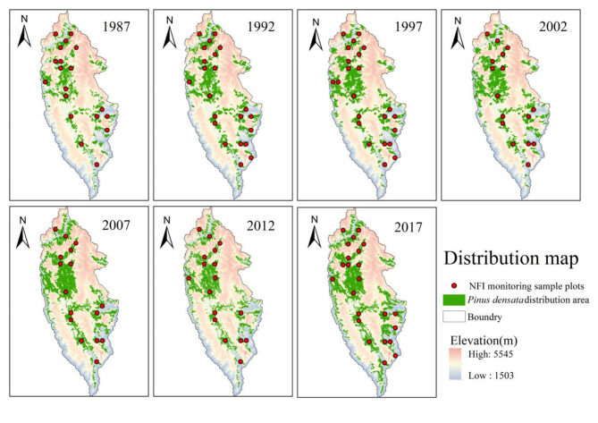
We employed the NFI data as the ground survey data collected in 1987, 1992, 1997, 2002, 2007, 2012, and 2017. The number of sample plots for Pinus densata measured in each year is as follows: 19, 22, 23, 16, 16, 17, and 23, totaling 136 plots, which include some remeasured plots. Each plot measures 28.28 m × 28.28 m and is recorded using the Beijing 54 coordinate system. The data includes average diameter at breast height (DBH), average tree height (H), and the number of Pinus densata. Due to the absence of 7 consecutive repeated measurements in some fixed plots, we selected 22 fixed plots with 7 consecutive repetitions as baseline data30. The distribution map of Pinus densata in Shangri-La was created by Yi Liao14 from our group using ArcGIS 10.8 based on Forest Management Inventory data. The distribution range of Pinus densata and the location of sample plots by year are shown in Fig. 11.
Fig. 11.
Sample plots and Pinus densata distribution map. The distribution map of Pinus densata was created by Yi Liao14 from our group using ArcGIS 10.8 based on Forest Management Inventory data.
Due to the difficulty in collecting understory vegetation and soil data, sample plots data is limited to aboveground components. Therefore, this study primarily focuses on the aboveground carbon sink. AGB of the sample plots was calculated using the anisotropic growth equation developed by the project team18. First, we calculated the average AGB using the average tree height and average diameter at breast height (DBH) of the plots. Then, we computed the total AGB of the plots based on the average AGB and the number of Pinus densata. The AGB equation was as follows:
 |
1 |
Where AGB stands for aboveground biomass (t), DBH stands for diameter at breast height (cm), H stands for tree height (m), and P is the number of Pinus densata.
We screened the sample plots data through the calculation results, in which 5 plots with too small AGB (AGB < 1 t·hm− 2) were excluded, and then 6 plots with outliers were screened and excluded according to Pauta’s criterion, in which a value is considered as an outlier if it exceeds three times the standard deviation of the mean value14. Finally, we can get 125 plots.
The AGCS of the sample plots was calculated by multiplying the AGB by the carbon content rate. According to the Guidelines for Carbon Stock Measurement in Forest Ecosystems issued by the State Forestry and Grassland Administration38, the average carbon content of Pinus densata dry matter was 0.501. The calculation formula was as follows:
 |
2 |
Where Cstock is the AGCS (t) in Pinus densata forest, and C is the carbon content rate.
The change of AGCS from year m to year n of the same plot is the aboveground carbon sink value of the plot during this period39. The formula is as follows:
 |
3 |
Where Csink is the aboveground carbon sink (t) in Pinus densata forest, and n and m denote the two different years, n > m.
The aboveground carbon sink can be divided by the area to obtain the carbon sink intensity (CSI). A positive value indicates a carbon sink, while a negative value signifies a carbon source40. Considering the significant differences in administrative areas among the townships in Shangri-La and the varying distribution ranges of Pinus densata, we adopted CSI as the standard so that the carbon sink capacity of Pinus densata in each township can be more objectively reflected.
Collection and processing of remote sensing data
We obtained Landsat 5 TM and Landsat 8 OLI time series images from the Geospatial Data Cloud website (https://www.gscloud.cn), covering 7 time periods and 21 views (Table 5). The spatial resolution of the images is 30 m. For each year, we selected the three images with the lowest cloud coverage to ensure minimal cloudiness in the chosen images.
Table 5.
Landsat time-series images.
| Sensor type | Year | Data identification | Stirp/Line | Acquisition time |
|---|---|---|---|---|
| Landsat5 TM | 1987 | LT51320401987364BKT00 | 132/40 | 30 December 1987 |
| 1987 | LT51310411987357BJC01 | 131/41 | 23 December 1987 | |
| 1987 | LT51320411987364BKT00 | 132/41 | 30 December 1987 | |
| 1992 | LT51320401991311BKT00 | 132/40 | 16 November 1991 | |
| 1992 | LT51310411991320BKT00 | 131/41 | 7 November 1991 | |
| 1992 | LT51320411991311BKT00 | 132/41 | 16 November 1991 | |
| 1997 | LT51320401997279BKT00 | 132/40 | 6 October 1997 | |
| 1997 | LT51310411997320BKT01 | 131/41 | 16 November 1997 | |
| 1997 | LT51320411997311BKT00 | 132/41 | 7 November 1997 | |
| 2002 | LT51320402002005BJC00 | 132/40 | 5 January 2002 | |
| 2002 | LT51310412002302BJC00 | 131/41 | 29 October 2002 | |
| 2002 | LT51320412002005BJC00 | 132/41 | 5 January 2002 | |
| 2007 | LT51320402007003BJC01 | 132/40 | 3 January 2007 | |
| 2007 | LT51310412007060BJC00 | 131/41 | 1 March 2007 | |
| 2007 | LT51320412006288BJC00 | 132/41 | 15 October 2006 | |
| 2012 | LT51320402011014BKT00 | 132/40 | 14 January 2011 | |
| 2012 | LT51310412011007BKT00 | 131/41 | 7 January 2011 | |
| 2012 | LT51320412011286BKT00 | 132/41 | 13 October 2011 | |
| Landsat8 OLI | 2017 | LC08_L2SP_132040_20171216_20200902_02_T1 | 132/40 | 16 December 2017 |
| 2017 | LC08_L2SP_131041_20171225_20200902_02_T1 | 131/41 | 25 December 2017 | |
| 2017 | LC08_L2SP_132041_20171216_20200902_02_T1 | 132/41 | 16 December 2017 |
To improve the image quality, we pre-processed all the images: firstly, the initial DN (digit number) values were converted to radiometric values using the Radiometric correction Tool to remove the effects of the sensors41; and atmospheric corrections were performed using the fast line-of-Sight Atmospheric Analysis of Spectral Hypercubes (FLAASH) module42. Then, geometric correction was performed on each image regarding the calibrated SPOT-5 image, the image coordinate system was corrected to the Beijing 1954 coordinate system to eliminate geometric errors, and the SPOT-5 image was resampled to a resolution of 30 m×30 m by bilinear interpolation to ensure that the error was less than 1 pixel; finally, terrain correction was performed using the slope matching model43. After terrain correction, the differences in radiance values of the images due to terrain relief are eliminated, and the images can better reflect spectral features14. Finally, the pre-processed images were stitched together by corresponding years.
To obtain the most relevant modeling factors for forest carbon sink, we extracted two types of remote sensing factors based on an extensive literature review14,30: spectral feature factors and texture feature factors. In total, 35 spectral factors and 540 texture factors (various types of textures computed from all single bands from 1 to 19 odd windows of each image) were extracted (Table 6).
Table 6.
Remote sensing factors information. B1 is the blue band, B2 is the green band, B3 is the red band, B4 is the near-infrared band, B5 is the shortwave infrared-1 band, and B7 is the shortwave infrared-2 band.
| Feature types | Factor types | Remote sensing factors |
|---|---|---|
| Texture features | Gray-level co-occurrence Matrix | Homogeneity (HO); Dissimilarity (DI); Mean (ME); Angular second moment (SM); Entropy (EN); Correlation (CC); Variance (VA); Contrast (CO) |
| Filtering of probabilistic statistics | Skewness (SK) | |
| Spectral features | General vegetation index factors |
NDVI = (B4 − B3)/(B4 + B3); ND32 = (B3 − B2)/(B3 + B2); ND54 = (B5 − B4)/(B5 + B4); ND53 = (B5 − B3)/(B5 + B3); ND57 = (B5 − B7)/(B5 + B7); ND452 = (B4 + B5 − B2)/(B4 + B5 + B2); DVI = B4 − B3; RVI = B4/B3; RVI = B4/B3; ARVI = (B4 − (2B3 − B1))/(B4 + (2B3 − B1)) |
| Information enhancement factors |
Principal component analysis (PCA1, PCA2, PCA3PCA4, PCA5, PCA7); VIS123 = B1 + B2 + B3; MID = B5 + B7; Albedo = B1 + B2 + B3 + B4 + B5 + B7; MID57 = B5 + B7 K-T |
|
| Simple ratio vegetation indices | B4/B2, B5/B3, B5/B4, B5/B7, B7/B3, B3/Albedo, B4×B3/B7 | |
| Original band factors | B1, B2, B3, B4, B5, B7 |
Collection and processing of meteorological data
The meteorological data includes the 1 km resolution monthly average precipitation dataset for China (1901–2022), the 1 km resolution monthly average temperature dataset for China (1901–2022), and the regional high-resolution (10 km) surface solar radiation dataset for China (1983–2017). These data were obtained from the National Tibetan Plateau Data Center (https://data.tpdc.ac.cn), with a horizontal accuracy of 30 m and a vertical accuracy of 20 m. To standardize the coordinate system and resolution with other datasets, the meteorological data were projected to the Beijing 1954 coordinate system and then resampled to a resolution of 30 m44.
Modeling process
We employed three types of variation to establish the carbon sink model: 5-year interval variation, 10-year interval variation, and annual average variation. The variation was based on two-year co-equal plots: we calculated the variation of the AGCS of the sample plots when the data were recorded in both calculation cycles, while the rest of the non-continuous samples we did not calculate14. In dynamic models, the variation in remote sensing factors was used as the independent variable and the variation of the AGCS as the dependent variable. The formulas for calculating the variations are as follows:
 |
4 |
 |
5 |
Where ∆V is the interval variation value, in which the variation is calculated, Vn and Vm are the data values of year n and year m, respectively, and ∆Va is the annual average change value.
The above two equations were used to calculate the AGCS variation and the variation of the corresponding remote sensing factors in each sample plots. The variation of AGCS was used as the CS value. The shortest time interval for calculating change data is 5 years, while the longest is 30 years. However, few continuous sample plots have time intervals of 15 years or more, and the sample size is insufficient to support the experiment.
We processed the 575 extracted remote sensing factors. After calculating their 5-year interval, 10-year interval, and annual average variation, Pearson correlation analyses were performed.
The effectiveness of the model during operation is influenced by the number of features. An excessive number of features can slow down model fitting, increase computational workload, and ultimately affect model stability10. The original features contain redundant information, which can decrease model accuracy and lead to adverse effects such as overfitting45. Conversely, too few variables can hinder the correct construction of the model. To avoid the risks of overfitting and covariance, we employed a stepwise regression method10. Following the methods of researchers14,30, we ultimately selected 10 strongly correlated remote sensing factors, all of which exhibited highly significant correlations (P < 0.01) for modeling.
RF is one of the most effective non-parametric regression models46. Compared to parametric regression methods, this method does not require testing assumptions such as the normality and independence of variables45. It can avoid overfitting, perform better with outliers, and handle high-dimensional data47. Additionally, it can assess the importance of each feature in the model. First, we need to adjust the model parameters, which include four key parameters: the maximum number of iterations (n_estimators), the maximum depth of the decision trees (max_depth), the minimum number of samples at leaf nodes (min_samples_leaf), and the minimum number of samples required to split an internal node (min_samples_split).
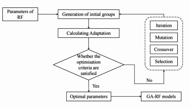
GA is an adaptive heuristic search algorithm that is part of evolutionary algorithms based on the principles of natural selection and genetics16. It applies to historical data provided by random searches to guide the search toward regions of the solution space that perform better. Typically, GA is used to generate high-quality solutions for optimization and search problems46, thereby avoiding the subjective tuning of hyperparameters associated with regular RF models. The primary operation process is divided into iterations, mutation, crossover, and selection.
Compared with regular RF models, GA assigns a weight vector to all variables in the feature space to evaluate their importance metrics16. By optimizing the parameter selection of RF using GA, we established the GA-RF models (Fig. 12). The main parameters involve four key components: population, iterations, mutation, and crossover.
Fig. 12.
Modeling process of the GA-RF.
The evaluation of model accuracy is divided into two parts: model fitting and model estimation effect test. 80% of the data were randomly selected for model fitting and 20% for the model estimation effect test for each model. The adopted model accuracy evaluation indexes include the coefficient of determination (R2), root mean square error (RMSE), relative root mean square error (rRMSE), and prediction accuracy (P). The calculation formulas are as follows48:
 |
6 |
 |
7 |
 |
8 |
 |
9 |
Where  represents the actual value,
  represents the model regression value,
 is the actual value mean, and n is the number of samples.
Analysis of driving forces
We used a correlation analysis method to calculate the degree of correlation between MAP, MAT, SSR, and forest CSI based on the pixel scale with the following equation49:
 |
10 |
Where Rxy represents the correlation coefficient of variables x and y, and its value range is [-1,1]. When the correlation coefficient is less than 0, it is called negative correlation; when it is greater than 0, it is called positive correlation. When it is equal to 0, it is irrelevant. The closer the absolute value is to 1, the stronger the correlation. xi is the CSI in the year i (t C·hm− 2), and yi is the climatic factor for year i.
In order to determine the effect of a single factor on CSI without interference from other factors, we used partial correlation analysis for further study50. The formula is as follows:
 |
11 |
Where  represents the first-order partial correlation coefficient between the CSI and the climatic factor y1 excluding the effect of climatic factor y2. To discuss the partial correlation coefficients between CSI and the three variables, the second-order partial correlation coefficient should be considered with the following formula5:
 |
12 |
Where  represents the second-level partial correlation coefficient between CSI and climatic factor y1 excluding the effect of climate factors y2 and y3. For example, the correlation between CSI and MAP after excluding the double effects of MAT and SSR.
The range of the partial correlation coefficient is also [-1,1]. Less than 0 indicates a negative correlation, more than 0 indicates a positive correlation, and the closer the absolute value is to 1, the closer the degree of partial correlation is.
The significance test was performed by the T-test with the following formula33:
 |
13 |
Where r is the partial correlation coefficient, n is the number of samples, 6(six periods), and m is the number of independent variables, 1. In this paper, the significance level of the t-test results was set at α = 0.0551. The correlation coefficients between CSI and climate factors were classified as highly significant (P < 0.01), significant (0.01 ≤ P < 0.05), and non-significant (P ≥ 0.05) according to the significance level.
The multi-correlation coefficient is an indicator that reflects the degree of correlation between a dependent variable and a set of independent variables (two or more). Moreover, it is a measure of the degree of multi-correlation51. The formula was calculated as follows:
 |
14 |
Where MR is the multi-correlation coefficient between the three climate factors and CSI, its value range is [0,1]. The larger the multi-correlation coefficient, the closer the linear correlation between the variables.
The significance test of the multi-correlation coefficient was performed by the F-test method with the following formula33:
 |
15 |
To accurately investigate the driving mechanisms of climate change on the CSI of Pinus densata in Shangri-La, we referenced the classification methods used by other researchers in Southwest China33,51. Subsequently, based on the significance analysis results of partial correlation and multi-correlation, we established the classification criteria for nine climate-driving factors (Table 7).
Table 7.
Rules of climactic driving factors for CSI of Pinus densata.
| Climate driving type | Criteria for classification | ||||
|---|---|---|---|---|---|
| Partial correlation coefficient | Multi-correlation coefficient | ||||
| PRCSI−Pre | PRCSI−Tem | PRCSI−SSR | MRCSI−Pre+Tem+SSR | ||
| Single-factor driver | MAP only | t < 0.05 | t ≥ 0.05 | t ≥ 0.05 | F < 0.05 |
| MAT only | t ≥ 0.05 | t < 0.05 | t ≥ 0.05 | F < 0.05 | |
| SSR only | t ≥ 0.05 | t ≥ 0.05 | t < 0.05 | F < 0.05 | |
| Double-factor driver | Double: MAP, MAT | t < 0.05 | t < 0.05 | t ≥ 0.05 | F < 0.05 |
| Double: MAP, SSR | t < 0.05 | t ≥ 0.05 | t < 0.05 | F < 0.05 | |
| Double: MAT, SSR | t ≥ 0.05 | t < 0.05 | t < 0.05 | F < 0.05 | |
| Triple-factor driver | Triple Strong Drive | t < 0.05 | t < 0.05 | t < 0.05 | F < 0.05 |
| Triple Weak Drive | t ≥ 0.05 | t ≥ 0.05 | t ≥ 0.05 | F < 0.05 | |
| Non-climatic driver | t ≥ 0.05 | t ≥ 0.05 | t ≥ 0.05 | F ≥ 0.05 | |
Implementation
In this study, Landsat time series images were pre-processed and remote sensing factors were extracted using ENVI 5.3 (https://envi.geoscene.cn/). SPSS 26.0 (https://www.ibm.com/cn-zh/products/spss-statistics) was used for Pearson analysis and feature screening of remote sensing factors and sample plots data. The resampling of meteorological data, the extraction of climate factors, the mapping of CS, and the analysis of driving forces, the above operations were finished on ArcGIS 10.8. Furthermore, in order to establish RF and GA-RF models and estimate CS, Anaconda3 (https://www.anaconda.com/) was used to build a Python 3.12 environment.
Acknowledgements
This work was funded by the National Natural Science Foundation of China (No. 32260390); “Young Top Talents” special project of the high-level talent training support program of Yunnan province, China, in 2020 (No. YNWR-QNBJ-2020-164); Innovation Programs of Southwest Forestry University (Grant No: LXXK-2023Z06).
Author contributions
K. Y. conceptualized the study, processed the data, designed the experiment and wrote the original draft. K.L. processed the data and analyzed results. J.Z. collected data, provided resources and edited the manuscript. B.Q. analyzed results. F.W., Q.X., J.C., Y.H. and J.Y. edited the manuscript. All authors reviewed the manuscript.
Data availability
The Landsat TM and Landsat OLI data are available through https://www.gscloud.cn/ (accessed on 23 October 2024) and The meteorological data are available through https://data.tpdc.ac.cn/home (accessed on 23 October 2024). NFI data presented in this study are available on request from the corresponding author; the data are not publicly available due to the confidentiality of the dataset.
Declarations
Competing interests
The authors declare no competing interests.
Footnotes
Publisher’s note
Springer Nature remains neutral with regard to jurisdictional claims in published maps and institutional affiliations.
References
- 1.Sun, X., Wang, G., Huang, M., Chang, R. & Ran, F. Forest biomass carbon stocks and variation in Tibet’s carbon-dense forests from 2001 to 2050. Sci. Rep.6, 34687. 10.1038/srep34687 (2016). [DOI] [PMC free article] [PubMed] [Google Scholar]
- 2.Cao, J., Tian, Y., Wang, X. & Sun, X. Estimation methods of forest sequestration and their prospects. J. Ecol. Environ.18, 2001–2005. 10.16258/j.cnki.1674-5906.2009.05.033 (2009). [Google Scholar]
- 3.Heinrich, V. H. A. et al. Large carbon sink potential of secondary forests in the Brazilian Amazon to mitigate climate change. Nat. Commun.12, 1785. 10.1038/s41467-021-22050-1 (2021). [DOI] [PMC free article] [PubMed] [Google Scholar]
- 4.Yang, Y. et al. Terrestrial carbon sinks in China and around the world and their contribution to carbon neutrality. Sci. China Life Sci.65, 861–895. 10.1007/s11427-021-2045-5 (2022). [DOI] [PubMed] [Google Scholar]
- 5.Liu, Z. & Chen, J. Correlation between temporal-spatial changes of vegetation and climate factors in Beijing. Geol. Notif.40, 2159–2166. 10.12097/j.issn.1671-2552.2021.12.018 (2021). [Google Scholar]
- 6.Liu, J. et al. Temporal and spatial variations of net primary productivity (NPP) and its climate driving effect in the Qinghai-Tibet Plateau, China from 2000 to 2020. J. Appl. Ecol.33, 1533–1538. 10.13287/j.1001-9332.202206.025 (2022). [DOI] [PubMed] [Google Scholar]
- 7.Takahashi, M. et al. Carbon stock in litter, deadwood and soil in Japan’s forest sector and its comparison with carbon stock in agricultural soils. Soil. Sci. Plant. Nutr.56, 19–30. 10.1111/j.1747-0765.2009.00425.x (2010). [Google Scholar]
- 8.Labrière, N. et al. Toward a forest biomass reference measurement system for remote sensing applications. Glob. Change Biol.29, 827–840. 10.1111/gcb.16497 (2023). [DOI] [PMC free article] [PubMed] [Google Scholar]
- 9.Chen, F., Yang, S., Yin, K. & Chan, P. Challenges to quantitative applications of landsat observations for the urban thermal environment. J. Environ. Sci.59, 80–88. 10.1016/j.jes.2017.02.009 (2017). [DOI] [PubMed] [Google Scholar]
- 10.Prăvălie, R. et al. Machine learning-based prediction and assessment of recent dynamics of forest net primary productivity in Romania. J. Environ. Manag.334, 117513. 10.1016/j.jenvman.2023.117513 (2023). [DOI] [PubMed] [Google Scholar]
- 11.Zhu, J. et al. Carbon stocks and changes of dead organic matter in China’s forests. Nat. Commun.8, 151. 10.1038/s41467-017-00207-1 (2017). [DOI] [PMC free article] [PubMed] [Google Scholar]
- 12.Huang, L. et al. Landsat-based spatiotemporal estimation of subtropical forest aboveground carbon storage using machine learning algorithms with hyperparameter tuning. Front. Plant. Sci.15, 1421567. 10.3389/fpls.2024.1421567 (2024). [DOI] [PMC free article] [PubMed] [Google Scholar]
- 13.Zeng, J. et al. The fusion of multiple scale data indicates that the carbon sink function of the Qinghai-Tibet Plateau is substantial. Carbon Balance Manag.1810.1186/s13021-023-00239-9 (2023). [DOI] [PMC free article] [PubMed]
- 14.Liao, Y., Zhang, J., Bao, R., Xu, D. & Han, D. Modelling the dynamics of carbon storages for Pinus densata using landsat images in Shangri-La considering topographic factors. Remote Sens.14, 6244. 10.3390/rs14246244 (2022). [Google Scholar]
- 15.Greener, J. G., Kandathil, S. M., Moffat, L. & Jones, D. T. A guide to machine learning for biologists. Nat. Rev. Mol. Cell. Biol.23, 40–55. 10.1038/s41580-021-00407-0 (2022). [DOI] [PubMed] [Google Scholar]
- 16.Xie, F., Zi, L. & Shu, Q. Optimizing the k-nearest neighbors technique for estimating Pinus densata aboveground biomass based on remote sensing. J. Zhejiang Agric. Forestry Univ.36, 515–523. 10.11833/j.issn.2095-0756.2019.03.012 (2019). [Google Scholar]
- 17.McDonnell, T. C. et al. Protection of forest ecosystems in the eastern United States from elevated atmospheric deposition of sulfur and nitrogen: A comparison of steady-state and dynamic model results. Environ. Pollut.318, 120887. 10.1016/j.envpol.2022.120887 (2023). [DOI] [PMC free article] [PubMed] [Google Scholar]
- 18.Zhang, J., Lu, C., Xu, H. & Wang, G. Estimating aboveground biomass of Pinus densata-dominated forests using landsat time series and permanent sample plot data. J. Res.30, 1689–1706. 10.1007/s11676-018-0713-7 (2019). [Google Scholar]
- 19.Gómez, C., White, J. C., Wulder, M. A. & Alejandro, P. Historical forest biomass dynamics modelled with Landsat spectral trajectories. ISPRS J. Photogramm. Remote Sens.93, 14–28. 10.1016/j.isprsjprs.2014.03.008 (2014). [Google Scholar]
- 20.Yu, K. et al. Pervasive decreases in living vegetation carbon turnover time across forest climate zones. Proc. Natl. Acad. Sci. U. S. A.116, 24662–24667. 10.1073/pnas.1821387116 (2019). [DOI] [PMC free article] [PubMed] [Google Scholar]
- 21.Fang, J., Yu, G., Liu, L., Hu, S. & S Chapin, F. Climate change, human impacts, and carbon sequestration in China. Proc. Natl. Acad. Sci. U. S. A.115, 4015–4020. 10.1073/pnas.1700304115 (2018). [DOI] [PMC free article] [PubMed] [Google Scholar]
- 22.Hubau, W. et al. Asynchronous carbon sink saturation in African and amazonian tropical forests. Nature579, 80–87. 10.1038/s41586-020-2035-0 (2020). [DOI] [PMC free article] [PubMed] [Google Scholar]
- 23.Xu, D. et al. Temporal and spatial variation of aboveground biomass of Pinus densata and its drivers in Shangri-La, CHINA. IJERPH19(400). 10.3390/ijerph19010400 (2021). [DOI] [PMC free article] [PubMed]
- 24.Teng, C., Zhang, J., Chen, Z., Bao, R. & Huang, K. Above-ground biomass estimation of Pinus densata based on landsat time series images and AHTC algorithm. J. Cent. South. Forestry Univ.44, 41–52. 10.14067/j.cnki.1673-923x.2024.02.005 (2024). [Google Scholar]
- 25.Illarionova, S. et al. Advancing forest carbon stocks’ mapping using a hierarchical approach with machine learning and satellite imagery. Sci. Rep.14, 21032. 10.1038/s41598-024-71133-8 (2024). [DOI] [PMC free article] [PubMed] [Google Scholar]
- 26.Zhang, X. et al. Research on the temporal and spatial distributions of standing wood carbon storage based on remote sensing images and local models. Forests13, 346. 10.3390/f13020346 (2022). [Google Scholar]
- 27.Li, X. & Zhang, X. A comparative study of statistical and machine learning models on carbon dioxide emissions prediction of China. Environ. Sci. Pollut Res.30, 117485–117502. 10.1007/s11356-023-30428-5 (2023). [DOI] [PubMed] [Google Scholar]
- 28.Xu, X. et al. Ecological engineering induced carbon sinks shifting from decreasing to increasing during 1981–2019 in China. Sci. Total Environ.864, 161037. 10.1016/j.scitotenv.2022.161037 (2023). [DOI] [PubMed] [Google Scholar]
- 29.Wang, J. et al. Maximizing the carbon sink function of paddy systems in China with machine learning. Sci. Total Environ.909, 168542. 10.1016/j.scitotenv.2023.168542 (2024). [DOI] [PubMed] [Google Scholar]
- 30.Han, D. et al. Improving Pinus densata carbon stock estimations through remote sensing in Shangri-La: A nonlinear mixed-effects model integrating soil thickness and topographic variables. Forests15, 394. 10.3390/f15020394 (2024). [Google Scholar]
- 31.Yin, T. et al. Estimating the Pinus densata carbon storage of Shangri-La by environmental variables. West. For. Sci.53, 119–128. 10.16473/j.cnki.xblykx1972.2024.01.015 (2024). [Google Scholar]
- 32.Peng, X. et al. Radial growth response of Pinus densata to climate factors in the Baima Snow Mountain, Northwest Yunnan. Acta Ecol. Sin.43, 8884–8893. 10.20103/j.stxb.202211143280 (2023). [Google Scholar]
- 33.Xu, Y. et al. Spatio-temporal variation of vegetation net ecosystem productivity and relative contribution of driving forces in Southwest China from 2000 to 2020. Environ. Sci.36, 557–570. 10.13198/j.issn.1001-6929.2022.12.01 (2023). [Google Scholar]
- 34.Tang, S. et al. Synergistic effects of multiple global change drivers on terrestrial ecosystem carbon sink. Sci. Total Environ.906, 167554. 10.1016/j.scitotenv.2023.167554 (2024). [DOI] [PubMed] [Google Scholar]
- 35.Liu, Y. et al. Evolution and assessment of forest carbon sink policy over the past 20 years. Ecol. J.43, 3430–3441. 10.5846/stxb202202110337 (2023). [Google Scholar]
- 36.Zhang, Y. et al. Extreme drought along the tropic of cancer (Yunnan section) and its impact on vegetation. Sci. Rep.14, 7508. 10.1038/s41598-024-58068-w (2024). [DOI] [PMC free article] [PubMed] [Google Scholar]
- 37.O’Sullivan, M. et al. Process-oriented analysis of dominant sources of uncertainty in the land carbon sink. Nat. Commun.13, 4781. 10.1038/s41467-022-32416-8 (2022). [DOI] [PMC free article] [PubMed] [Google Scholar]
- 38.Wang, J. et al. Carbon content rate in dominant species of four forest types in Shangri-la,northwest Yunnan Province. J. Ecol. Environ.21, 613–619. 10.16258/j.cnki.1674-5906.2012.04.010 (2012). [Google Scholar]
- 39.Huang, C., Zhang, Z., Zhang, W. & Yang, J. A. Review of overseas remote sensing monitoring methods for aboveground forest carbon sink. World For. Res.25, 20–26. 10.13348/j.cnki.sjlyyj.2012.06.008 (2012). [Google Scholar]
- 40.Cui, Y., Khan, S. U., Sauer, J. & Zhao, M. Exploring the spatiotemporal heterogeneity and influencing factors of agricultural carbon footprint and carbon footprint intensity: Embodying carbon sink effect. Sci. Total Environ.846, 157507. 10.1016/j.scitotenv.2022.157507 (2022). [DOI] [PubMed] [Google Scholar]
- 41.Wu, W. et al. A long time-series radiometric normalization method for landsat images. Sensors18, 4505. 10.3390/s18124505 (2018). [DOI] [PMC free article] [PubMed] [Google Scholar]
- 42.Nguyen, H. et al. Optimal atmospheric correction for above-ground forest biomass estimation with the ETM + remote sensor. Sensors15, 18865–18886. 10.3390/s150818865 (2015). [DOI] [PMC free article] [PubMed] [Google Scholar]
- 43.Gao, Y. & Zhang, W. L. U. L. C. Classification and topographic correction of Landsat-7 ETM + imagery in the Yangjia River Watershed: The influence of DEM resolution. Sensors9, 1980–1995. 10.3390/s90301980 (2009). [DOI] [PMC free article] [PubMed] [Google Scholar]
- 44.Moisen, G. G. et al. Shape selection in Landsat time series: A tool for monitoring forest dynamics. Glob. Change Biol.22, 3518–3528. 10.1111/gcb.13358 (2016). [DOI] [PubMed] [Google Scholar]
- 45.Canero, F. M., Rodriguez-Galiano, V. & Aragones, D. Machine learning and feature selection for soil spectroscopy. An evaluation of random forest wrappers to predict soil organic matter, clay, and carbonates. Heliyon10, 30228 (2024). 10.1016/j.heliyon.2024.e30228 [DOI] [PMC free article] [PubMed] [Google Scholar]
- 46.Goldstein, B. A., Polley, E. C. & Briggs, F. B. S. Random forests for genetic association studies. Stat. Appl. Genet. Mol. Biol.10, 32. 10.2202/1544-6115.1691 (2011). [DOI] [PMC free article] [PubMed] [Google Scholar]
- 47.Araza, A., De Bruin, S., Hein, L. & Herold, M. Spatial predictions and uncertainties of forest carbon fluxes for carbon accounting. Sci. Rep.13, 12704. 10.1038/s41598-023-38935-8 (2023). [DOI] [PMC free article] [PubMed] [Google Scholar]
- 48.Liao, Y., Zhang, J., Bao, R. & Xu, D. Estimating the dynamic changes of aboveground biomass of Pinus densata based on Landsat. J. Southwest. For. Univ. (Nat. Sci.)43, 117–125. 10.11929/j.swfu.202111058 (2023). [Google Scholar]
- 49.Huang, K. et al. Effects of land use and climate change on spatiotemporal changes of evapotranspiration in haihe river basin. J. Earth Inf. Sci.21, 1888–1902 (2019). 10.12082/dqxxkx.2019.190269 [Google Scholar]
- 50.Wang, Y., He, J., He, L., Zhang, Y. & Zhang, X. Vegetation phenology and its response to climate change in the Yellow RiverBasin from 2001 to 2020. Acta Ecol. Sin.44, 844–857. 10.20103/j.stxb.202302220311 (2024). [Google Scholar]
- 51.He, Y. et al. The EVl trends and driving factors in Red River Basin affected by the ‘corridorbarrier’ function during 2000–2014. Acta Ecol. Sin.38, 2056–2064. 10.5846/stxb201703210483 (2018). [Google Scholar]
Associated Data
This section collects any data citations, data availability statements, or supplementary materials included in this article.
Data Availability Statement
The Landsat TM and Landsat OLI data are available through https://www.gscloud.cn/ (accessed on 23 October 2024) and The meteorological data are available through https://data.tpdc.ac.cn/home (accessed on 23 October 2024). NFI data presented in this study are available on request from the corresponding author; the data are not publicly available due to the confidentiality of the dataset.


