

Abstract
This study presents a novel approach to identifying meters and their pointers in modern industrial scenarios using deep learning. We developed a neural network model that can detect gauges and one or more of their pointers on low-quality images. We use an encoder network, jump connections, and a modified Convolutional Block Attention Module (CBAM) to detect gauge panels and pointer keypoints in images. We also combine the output of the decoder network and the output of the improved CBAM as inputs to the Object Heatmap-Scalarmap Module to find pointer tip heat map peaks and predict pointer pointing. The method proposed in this paper is compared with several deep learning networks. The experimental results show that the model in this paper has the highest recognition correctness, with an average precision of 0.95 and 0.763 for Object Keypoint Similarity and Vector Direction Similarity, and an average recall of 0.951 and 0.856 in the test set, respectively, and achieves the best results in terms of efficiency and accuracy achieve the best trade-off, and performs well in recognizing multiple pointer targets. This demonstrates its robustness in real scenarios and provides a new idea for recognizing pointers in low-quality images more efficiently and accurately in complex industrial scenarios.
Subject terms: Computer science, Information technology, Software
Introduction
Although significant progress has been made in high-performance target detection models in recent years, the detection performance can be severely degraded when the image quality deteriorates1. Currently, there are fewer detection methods for pointer meters and an uncertain number of pointers in the industrial field. This study aims to address these issues by proposing a model based on convolutional networks. Compared to existing methods, our model reduces the computational complexity while still maintaining a high level of detection performance on the publicly available dataset and the subset of low-quality images categorized from it. The contribution of this paper is that our method can still accurately and efficiently recognize indeterminate pointers in low-quality images in complex industrial environments, and experimentally validate the method’s effectiveness in real-world applications. Pointer meters are widely used in the industrial field due to their advantages of low manufacturing cost, wide applicability, high accuracy, fast response, and high sensitivity2. Inspection and condition monitoring in complex industrial scenarios, such as substations3, nuclear power plants4, and gas stations5, have a vital and critical impact on the level of operation and safe and stable operation in these scenarios. However, due to the lack of digital communication serial ports, the data of these instruments are mainly based on the traditional manual inspection method6, which requires a lot of labor and time costs, and there are fault hazards of false alarms and high omission rate. Moreover, some scenes are in high radiation, high altitude, high temperature, and other complex environments, where the traditional manual inspection method cannot comprehensively, accurately, and timely collect instrument data. This causes problems such as large reading errors and labor intensiveness, which puts enormous pressure on grassroots staff. In recent years, with the rise of machine learning and the rapid development of computer vision technology, artificial intelligence technology has gradually emerged, and machine vision has begun to gradually replace the human eye for target detection in images7. This trend indicates that automated image processing and target detection systems are gradually replacing traditional manual observation and analysis methods8. Therefore, it is of great practical importance to rely on inspection robots and computer vision techniques for automated meter reading9–11, which may ultimately reduce production costs and increase productivity.
In order to improve the efficiency of pointer detection and reduce the cost of manual patrol, we propose to use deep learning techniques to solve the above tasks. Camera devices and patrol robots within the industrial scene are utilized to capture meter images and automatically detect and identify pointers within the meters in the images. There are three main difficulties in automatic recognition of meter pointers. The first is to distinguish the complex background from the dial area. Then the number of pointers in different types of meters is not the same, the scale and pointer color may be similar, there is the possibility of missed or misdetection, increasing the difficulty of pointer recognition. Due to the fact that some of the camera equipment is old and the images captured are of low resolution, or the meters are tilted and poorly illuminated due to different shooting angles and brightness, how to accurately recognize the pointers in these low-quality images is also one of the difficulties. However, existing conventional methods often struggle to accurately identify the meter and all the pointers therein on low-quality images. Aiming at the above three technical challenges, an instrument pointer recognition method based on target keypoint detection is proposed, which employs a deep learning model in detection and recognition. The model consists of an encoder network, an improved Convolutional Block Attention Module (CBAM), a decoder network, and an Object Heatmap-Scalarmap Module (OHSM) designed by us, all of which guarantee accuracy and robustness in natural scenes. The robustness of the model is demonstrated by its ability to train the model on different types of low-quality images with improved recognition accuracy. By advancing this technology, the pressure of manual inspection in complex industrial scenarios can be reduced and inspection efficiency can be improved.
Briefly, in this paper, we make the following contributions:
We design and implement a learning-based, robust end-to-end system for automatically detecting pointers in pointer meters and recognizing their orientations. Experiments demonstrate that our designed network improves the accuracy of pointer recognition in meters.
In addition, facing the challenges of low-quality images (low resolution, scaling, and under poor lighting conditions), our designed network still has high accuracy. Experiments demonstrate that our designed network improves the accuracy of in-meter pointer recognition in low-quality images.
Comprehensive experimental comparisons of our approach with multiple image segmentation baselines show that our model can quickly read and accurately automatically recognize not only individual meter pointers, but also multiple pointer targets in a meter.
Due to our innovative approach, comprehensive experimental comparisons with multiple image segmentation baselines show that our model recognizes meter pointers in images in real time.
Therefore, this study aims to address the problem of accurately and efficiently identifying pointers in low-quality images in complex industrial scenarios. Specifically, we propose a learning-based robust end-to-end training model to reduce computational complexity while maintaining high detection accuracy. The novelty of this study lies in applying our proposed improved CBAM and OHSM methods to the model architecture and experimentally demonstrating their superior performance. Through this research, we provide a new solution for accurately and efficiently recognizing pointers in low-quality images in complex industrial scenarios.
The rest of the paper is organized as follows: in Section "Related work" we provide relevant background knowledge. In Section "Method" we describe the proposed pointer detection and recognition method in detail. In Section "Experiments", we evaluate the performance of the proposed method through extensive simulation experiments and ablation studies. Finally, the conclusion of this paper is presented in Section "Conclusion".
Related work
Until now, numerous researchers have proposed methods for pointer meter detection and recognition, which can be broadly categorized into the following two groups. Figure 1 illustrates the common steps of these two groups of methods.
Fig. 1.

Pointer meter detection and recognition methods.
Traditional machine learning
Traditional machine learning methods were once widely used for target detection tasks. These methods are mainly based on the combination of feature engineering and classifiers, and the process usually includes feature extraction, feature selection, and classifier training. Commonly used features include Histogram of Oriented Gradients (HOG), and Scale Invariant Feature Transform (SIFT)12,13. These hand-designed features capture edge information or local patterns in the image. To determine the presence of the target object in the detection window, classifiers such as Support Vector Machine (SVM) are often used14. Traditional machine learning methods perform better on small-scale datasets, but their performance relies heavily on hand-designed features, resulting in poor model generalization. In addition, when the amount of data or the complexity of the task increases, there is a large gap in the performance of these methods compared to modern deep learning15,16.
In some complex instrumentations, it is difficult to accurately detect pointers by relying only on the Hough transform. So K-Nearest Neighbors (KNN) or other more advanced methods are needed to categorize the pointer and non-pointer regions in the detection region17. Such classifiers can be trained to adapt better to different types of pointers and dials. In critical industrial scenarios, using machine learning techniques for meter monitoring can reduce manual errors and improve efficiency. However, these methods typically require large amounts of manually labeled data for training and have limited ability to generalize across different types of gauges. For example, variations in the design of different dials or the material of the pointer may affect the accuracy of the detection18. In addition, traditional machine learning methods are not robust to noise and light variations, especially in harsh environments such as high temperature and high humidity, where the recognition performance is significantly degraded19.
Detection method based on deep learning
In order to cope with the challenges posed by traditional change detection methods, new methods utilizing deep learning techniques have emerged in recent years, especially deep convolutional neural networks (CNNs)20,21. By utilizing the powerful computational capabilities of CNNs, these methods can efficiently extract complex spatial features from paired images captured at different times, allowing for more accurate and detailed detection of changes in the scene22,23. The R-CNN family of models pioneered the combination of target detection and region extraction, of which R-CNN, Fast R-CNN, and Faster R-CNN are widely used in detection tasks24,25. However, the detection speed of these models is slow and cannot meet the demand of real-time applications. To improve detection efficiency, YOLO (You Only Look Once) series models and SSD (Single Shot Detector) realize real-time detection through an end-to-end structure, which is widely used in the fields of traffic monitoring and drone surveillance26–29. These models can maintain high accuracy while reducing computational costs through the improvement of network structure. In recent years, Vision Transformer (ViT) and DETR (Detection Transformer) models have achieved higher detection performance by the self-attention mechanism.DETR eliminates the traditional anchor frame design and performs outstandingly in complex scenes30. These advances lay the foundation for fine-grained detection tasks, such as pointer detection in dashboards.
In the industrial sector, such as power plants and chemical plants, pointer gauges are key devices for monitoring important parameters such as temperature and pressure. In order to realize automated monitoring and fault detection, several deep learning-based detection schemes have emerged in recent years. CNN models are used to extract the pointer and scale information of instrument panels, and automated detection is realized through image preprocessing and feature learning. For example, researchers have detected the position and pointer angle of gauges through YOLO or SSD models to realize unattended monitoring31.These models have good performance in simple environments, but their performance is not stable enough in the case of lighting changes or diverse pointer materials. For the detection needs in complex industrial scenarios, some research has attempted to use the Transformer architecture for pointer gauge recognition. These models can better capture global information and are especially suitable for dealing with noisy or blurred pointers32. Meanwhile, the use of the attention mechanism can improve the robustness of the detection model under high temperature or light change conditions.
In the above studies, most of the studies were unable to accurately recognize the pointers in the meter in low quality images. Although the traditional methods are more efficient, the accuracy rate is lower than the deep learning methods. Secondly, in real scenarios, when there are multiple pointer targets in the meter, these methods are still unable to recognize them comprehensively, and there is a high leakage rate. However, in terms of real-time, most of these methods are unable to meet the demand for real-time detection and recognition in real scenarios. To address the above problems, our proposed method, convolutional neural network model, can achieve accurate recognition of multiple pointer targets in high and low quality images faster.
Method
In this section, our pointer detection method Pointer Indication Network (PIN) is described in detail in subsections "Pointer Indication Network (PIN)", Training process, and Loss function, describing its network architecture, training, and loss function, respectively. Figure 2 shows the proposed model used in this study.
Fig. 2.

Proposed model.
Pointer indication network (PIN)
Figure 3 illustrates the network framework of PIN. The network framework of PIN can be represented as , which consists of an encoder network E, an improved Convolutional Block Attention Module (CBAM)33 A, a decoder network D, and a target heatmap- scalarmap module, OHSM) O. Given a two-dimensional input image x of size (w is the width and h is the length), the heatmap output and scalarmap output can be computed by:
| 1 |
where and are the low-level information generated by the first encoder and the second encoder of the encoder network E, respectively, which contain less semantic information, and it is easy for gradient explosion to occur by using them directly as the feature detection layer34,35. Therefore, these two low-level information layers are jump-connected into the improved CBAM to enrich the shallow high-resolution, low semantic feature information, solve the shallow feature information loss problem, and improve the convergence speed of the model36. The following points describe each operation.
Fig. 3.

An illustration of the PIN architecture. There is fully convolutional network. The input image is first processed by five encoders of the Encoder Network, then three decoders of the Decoder Network upsample its input to increase the resolution of feature maps and the spatial dimension of extracted features. Finally, the final decoder output feature maps are fed to the object heatmap-scalarmap module to predict a confidence heatmap and two scalar maps for pointer recognition, respectively.
Encoder network E: In order to avoid layer-by-layer feature disappearance and accuracy degradation as the network depth increases, each encoder of the encoder network employs a ResBlock37 with a residual structure, as shown in Fig. 4. The encoder network consists of 49 convolutional layers, corresponding to the first 49 convolutional layers in the ResNet50 network37. Downsampling allows deeper layers of the network to gather contextual informa-tion while helping to reduce the amount of computation. The output of the encoder is and x is the input of the previous layer. A maximum pooling layer is inserted between the first encoder and the second encoder for achieving translation invariance over small spatial shifts in the input image, which is more robust. Batch normalization (BN)38 is applied to the encoders after each time they perform convolution with the filter bank to produce a set of feature maps. When the inputs and outputs of ResBlock have the same dimensions, identity shortcuts can be used directly (solid line shortcuts in Fig. 4). And when the dimensions do not match (dotted line shortcuts in Fig. 4), the matching of input and output dimensions is accomplished by convolution. When shortcuts pass through feature maps of different dimensions, they have a step size of 2. An element-by-element Rectified Linear Unit (ReLU)39 is applied after the shortcuts:
Fig. 4.

Architecture details of Encoder Network. The CBR consists of a convolutional layer, batch normalization and ReLU activation function. Except for the first encoder which has a convolution kernel size of , the other encoders all have a convolution kernel size of and shortcut connection.
| 2 |
where p is the output produced by two feature maps performing element-by-element summation on a channel-by-channel basis. The purpose of using an encoder cascade is to capture a large enough receptive field to capture semantic contextual information and learn rich information between pixels within an image for pixel-level prediction.
In order to reduce the number of model parameters and computation, in the encoder network, we reduce the number of channels in the convolutional layer, thus reducing the computational overhead of the model without significantly degrading the model performance, shrinking the model size, reducing the use of runtime memory, and improving the inference speed to make it suitable for real-time applications40,41. We also keep the number of convolutional layer channels in each CBR constant to optimize network performance and reduce model complexity. Keeping the number of channels consistent reduces the complexity of feature transformation, which indirectly improves training and inference efficiency42,43.
-
(2)
Improved CBAM: CBAM (Convolutional Block Attention Module) is a simple but effective feed-forward convolu-tional neural network attention module. Attention not only tells us where to focus, but also improves the expression of interest44,45. The module focuses on important features and ignores unnecessary features by using the attention mechanism.CBAM contains two sub-modules, the channel attention module46 and the spatial attention module47,48. The channel attention module learns the “what” to focus on in the channel axis, and the spatial attention module learns the “where” to focus on in the spatial axis. Combining these two modules, by learning to emphasize or suppress information, it effectively helps the network to improve the representation of the target and enhance saliency feature extraction. The structure of the improved CBAM is shown in Fig. 5. In the improved CBAM, the spatial and channel attention modules are applied sequentially to help the network pay more attention to the targets in the intermediate feature map. In complex industrial scenarios, the pointer inside the dashboard is very tiny for the whole image, and such a detail is difficult to be attended to by an ordinary network. Therefore the attention mechanism is needed to amplify the network’s attention and learning effort on it. By inserting this module, a higher accuracy than the baseline network was obtained in the Pointer-10K dataset49 (see Section "Experiments and result"). Since the module is lightweight, the overhead of parameters and computation is negligible in most cases.
Fig. 5.

The overview of improved CBAM. Two sequential sub-modules in the module: spatial and channel. We feed the input intermediate feature map to our module(improved CBAM) and obtain the weighted feature maps.
As shown in Fig. 5, given the intermediate feature map as input, the improved CBAM uses the spatial attention module to obtain the spatial attention weight , which is multiplied by and I to obtain the spatial weighted feature map . Pass it to (feed ... to) the channel attention module to obtain the channel attention weight , and multiply WC and to obtain the channel weighted feature map . The process can be summarized as:
| 3 |
where denotes element-by-element multiplication. During multiplication, spatial attention is propagated along the channel dimension, and channel attention is propagated along the spatial dimension. is the output of the improved CBAM. Figure 6 depicts the computation process of each attention map.
Fig. 6.

Diagram of spatial and channel attention sub-module. As shown, the spatial sub-module selects the maximum and average values in all channel dimensions and forward them to a convolution layer to generate spatial attention weights; the channel sub-module utilizes max pooling and average pooling with a shared MLP to generate the channel attention weight.
Improved spatial attention module
In general, the content of interest is only relevant to some regions of the image. Therefore, the spatial attention mechanism is utilized to try to pay more attention to semantically relevant regions rather than paying the same attention to every region in the image. To obtain the spatial attention weights, the maximum and average values are first computed on the channel dimension and they are concatenated to generate spatially rich feature representations. Pooling operations on the channel dimension can significantly improve the performance of convolutional neural networks (CNNs) and effectively highlight the semantically informative regions of attention50. Applying a convolutional operation on the cascaded feature representations generates the spatial attention weight , which emphasizes the location of interest and suppresses other regions. The detailed operations are described next.
The spatial information of the feature maps is obtained by using the maximum pooling and average pooling operations to generate two 2D feature maps and , which represent the maximum pooled and average pooled features of the feature maps over all channels, respectively. They are then concatenated and convolved through a convolutional layer to generate 2D spatial attention weights. Briefly, the spatial attention weights are computed as follows:
| 4 |
where denotes a convolution operation with a convolution kernel size of , and denotes the tanh function, which is used to generate spatial attention weights on the feature map region. The reason for using the tanh function instead of the sigmoid function is that the sigmoid function converges slowly, and the tanh function solves this problem. The spatial attention weights are multiplied element by element with the input feature map to obtain a spatially weighted feature map.
Improved channel attention module
The channels in the feature map reflect the feature information in the foreground and background. Therefore, the channel attention mechanism is utilized to try to pay more attention to the feature information of interest rather than paying the same attention to each channel in the feature map. After obtaining the spatially weighted feature map , where denotes the jth channel in the feature map and C is the number of channels, the channel attention weights are generated by exploiting the inter-channel relations of the feature map.Each channel of the feature map output by the CNN can be used as a separate feature extractor51, and thus channel attention can be viewed as the process of selecting, given an input image, the process of semantic attributes. Channel attention is complementary to spatial attention in that they focus on different parts of the information. We use maximum pooling and average pooling for each channel to obtain important cues about the features of the object of interest, avoiding cue omissions that lead to coarse channel attention.The detailed operations are described next.
Channel features are first obtained using maximum pooling and average pooling operations for each channel:
| 5 |
where scalar is the maximum value of vector and scalar is the mean value of vector , denoting the jth channel feature. The and denote the maximal channel merging feature descriptor and the average channel merging feature descriptor, respectively. These two descriptors are transmitted to a shared multilayer perceptual machine (MLP) to generate the channel attention weights . The MLP consists of multiple hidden layers, and the hidden layer activation applies the Leaky ReLU function, which is used to solve the neuron necrosis problem of ReLU. To prevent excessive parameter overhead, the hidden layer activation size is set to , where r is the reduction ratio. after the MLP is applied to each descriptor, channel attention weights are merged and output using element-by-element summation. Briefly, the channel attention weights are computed as follows:
| 6 |
where denotes the tanh function, which is used to generate the channel attention weights on the feature map region. Note that the MLP weights are shared for both inputs. The channel attention weights are multiplied element-by-element with the sum spatially weighted feature map to obtain the output of the improved CBAM, which is used as an input to the decoder D.
-
(3)
Decoder Network D: Decoders in the decoder network up-sample coarse spatial and strong semantic feature maps from the encoder. The high-level abstract features are generated into high-resolution decoder-dense feature maps by back-convolution, and then batch normalization and ReLU are applied to each map.The decoder outputs a high-dimensional feature representation enriched with global contextual and semantic information, which is sent to the target heatmap-scalar map module. The encoder network and decoder network are thus asymmetric due to the non-consistent input and output sizes of the PIN.
-
(4)
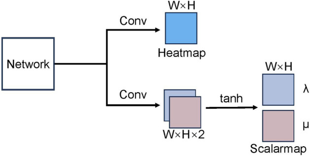
Object Heatmap-Scalarmap Module (OHSM) O: Inspired by ECA-Net52, a channel attention mechanism is introduced to enhance the extraction of features and further improve the performance of our deep CNN model, PIN, due to the small representation of pointers in the image and the over-representation of the background53,54. Since dimensionality reduction imposes side effects on channel attention prediction and capturing the dependencies between all channels is inefficient and unnecessary52, our proposed OHSM avoids dimensionality reduction and employs an efficient way to capture correlations between channels as a means of generating heat maps highlighting the location of the pointer head and scalar maps predicting where the pointer is pointing. Channel dependency causes each convolutional filter to operate using only the local receptive field, and is unable to utilize contextual information outside of that region. To address this problem, we use channel average pooling without dimensionality reduction to compress global spatial information into channel descriptors and efficiently capture correlations between local channels by considering each channel and its k neighbors.
As shown in Fig. 7, the result obtained by the element-by-element summation of the output of the improved CBAM and the output of the decoder network serves as the input to our OHSM.The weights of the channels in the OHSM can be expressed as
| 7 |
where is the global channel average pooling, is the sigmoid function, and our OHSM uses the banding matrix to learn channel attention:
| 8 |
in Eq. (8) involves , avoiding complete independence between the different groups in the equation. Let , the weight of in Eq. (8) is calculated by considering only the correlation between and its k neighbors:
| 9 |
where denotes the set of k neighboring channels of , all of which share the same learning parameters.
Fig. 7.

Diagram of our object heatmap-scalarmap module(OHSM). OHSM has two branches. One branch is to generate a heat map by performing a convolution operation with given feature maps. The other branch is to obtain comprehensive features by global average pooling, generate channel weights by performing 1D convolutions of size k, multiply them element-wise with the input, and then generate scalar maps by convolution operation and tanh activation function.
We implement the above strategy using a one-dimensional convolution with kernel size k:
| 10 |
where 1D denotes one-dimensional convolution, only k parameters are involved in Eq. 10, which ensures very low module complexity and negligible computational effort, while at the same time providing a significant improve-ment in performance by capturing local channel correlations to learn effective channel attention.
This module enhances the ability to extract shallow feature information, and improves the accuracy of pointer key point and direction recognition and enhances the detection effect by fusing the high resolution of shallow features and the high semantic information of higher-level features.
Our PIN is a fully convolutional network (FCN) with dual outputs that can be trained end-to-end. Convolutional neural networks (CNNs) have been shown to be very effective in various domains55,56, mainly due to the fact that
Feature information in data is extracted by a learnable convolutional kernel with the possibility of parameter sharing, which gives the network better feature extraction,
The use of stochastic gradient descent (SGD) optimization to learn domain-specific image features,
The ability to perform translation invariance on information such as images. In particular, Fully Convolutional Networks (FCNs)57, e.g.,58–60 have been shown to achieve robust and accurate performance in image segmentation tasks.
Training process
Given a set of RGB image blocks , we iteratively take , and in the training phase, PIN takes as input after affine transformation and produces a set of confidence coefficients representing the direction of the pointer units as output. Let
| 11 |
is the detection result of the ith pointer, where is the initial coordinate point; are the scalar components on the X-axis and Y-axis, respectively; is the confidence coefficient, , and is the number of pointers detected in the image.
Note that the number of pointers for a known category meter is known in advance, but PIN itself is unknown about , and it only outputs a determined confidence level for the pointers. The number of pointers output by PIN may be less than or equal to due to pointers overlapping each other or pointers overlapping the scale leading to pointers being incorrectly identified as non-pointers.Our PIN predicted heat map  and scalar map regress to the ground truth heat map
  and the ground truth scalar map , respectively.If in exceeds a confidence threshold, then the peak in
  is used as the pointer tip, where , . Scale the coordinates of this peak in
  back to . We assign the values at the coordinates of the two channels in to and , respectively.
For the ground truth heat map  , we consider the tips of the pointers to be more defined and easy for the network to localize them, while other parts of the pointers (e.g., the tails) may be coarse, which makes them difficult to be labeled. We initialize
  using a blank map filled with zeros, and for each pointer tip pixel point , we scale it to , and compute the value of each pixel in
  by applying a 2D Gaussian distribution centered on :
 |
12 |
where is the standard deviation controlling for the width and kurtosis of the distribution curve.
For a ground truth scalar map , we denote the pointer’s pointing direction by a blank map and of the same size as  , respectively, where and denote the two scalar components of the pointer. We derive their values for each pixel recursively:
| 13 |
where , and denote the two channel indication values of the ith pointer at pixel for , respectively. Then
| 14 |
where , superimposing and along the channel gives :
| 15 |
Loss function
The training objective of PIN is to minimize the mean square error (MSE) loss between the predicted heat map  and the ground truth heat map
  , denoted by
  , and the MSE loss between the predicted scalar map and the ground truth scalar map , denoted by . The overall loss with respect to the training epoch is
| 16 |
where Z is the total training epoch and is the epoch index. we observe that converges slower than  , which tends to make the PIN fall into a local maximum if no special treatment is performed. Empirically, the semantic information at the tip of the pointer is more easily utilized by the network, while the direction indicated by the pointer is not significant for scalar graphs. Therefore, we use , , and to balance the relationship between
  and , which enables PIN to find the pointer tip and the indicated direction faster.
This study improves the safety and efficiency of inspections in industry and has significant social value. In critical environments such as power plants and chemical plants, auto-detecting pointer-type meters and pointers can reduce the reliance on manual inspection, thereby minimizing human error and associated safety risks. One of the key determinants in evaluating the success of a proposed system is the accuracy and speed of detection under varying environmental conditions. Higher detection accuracy and faster detection speeds ensure that faults are recognized and potential disasters and equipment failures are prevented. Additionally, the study demonstrates greater robustness to environmental changes, such as changes in lighting or image sharpness, which are common challenges in industrial environments. By integrating advanced deep learning techniques, this research contributes to automating industrial tasks, ultimately reducing operational costs and improving resource management. In the long run, the proposed system supports sustainable industrial growth by optimizing performance, thereby benefiting society as a whole through safer and more efficient infrastructure.
Experiments and results
Dataset
We benchmarked the performance of PIN on the Pointer-10K49 dataset from https://github.com/DrawZeroPoint/VectorDetectionNetwork. The dataset contains 5,440 RGB instrument images with a resolution of 1280 720 and about 10,000 pointer instances, of which 1/3 are industrial instrument images in real scenes, 1/3 are industrial instrument images with manually adjusted pointers, and the other 1/3 are industrial instrument images obtained from the Internet. As shown in Fig. 8, the dataset provides each pointer with the instrument bounding box and the three key points of the pointer tip, midpoint and tail. The dataset is used for train, validation and test in the ratio of 7:2:1, and there are 3806, 1083 and 539 images in the three parts of train, validation and test, respectively, where the train part is used for training, and the validation and test parts are used for the performance testing and ablation experiments. As shown in Fig. 9, some of the images are deliberately blurred, scaled, or have poor lighting conditions, and such processing makes the trained network more robust to processing real-world scenes.
Fig. 8.
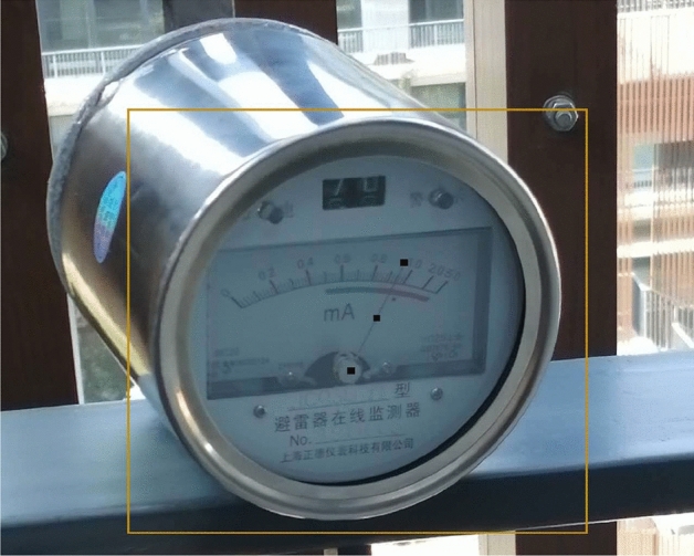
Annotation of the sample image. The image is from49.
Fig. 9.
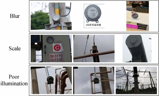
Low quality images in Pointer-10K49 (blur, scale, and poor illumination).
In order to highlight the superiority of our proposed method in recognizing multi-pointer targets in pointer meters, we selected images containing multi-pointer targets in the test part of the Pointer-10K49, called the multiple pointer targets dataset (MPT). Meanwhile, in order to show the superiority of our proposed method in recognizing pointer targets in low-quality images, we selected images with blurring, scaling, and poor lighting conditions in the TEST portion of the Pointer-10K49, called the low quality pointer images dataset (LQPI).
Implementation details
In our study, the models are trained and tested using an Ubuntu implementation with the following specifications. The Graphics Processing Unit (GPU) is an NVIDIA Tesla V100, and the deep learning framework is PyTorch 1.10.We set the input image size to 384 384 pixels, the batch size to 8, the momentum size to 0.9, and the epoch to 100. During training, the cost function is optimized using the Adam optimizer71, and the learning rate is initialized to using an on-demand tuning strategy. The learning rate is reduced at the 70th and 90th epochs with the decay coefficient set to 0.1. our backbone is ResNet50 initialized by a model pre-trained on the ImageNet classification task72. is set to 3 in Eq. (12), is set to 1 in Eq. (16), is set to 0.8, and set to 1 (see Section "Parameterization"). After the model training was completed, a pytorch model of size 110 MB was obtained.
Evaluation results
Given the similarity between biomedical images and instrumented images68, our proposed PIN is compared with several image segmentation networks, including VDN49, Anam-Net61, UNet62, UNet++63, SegNet64, Enet65, LEDNet66, improved Unet++67 and improved U-Net68, which are used as baseline methods to demonstrate the real-time performance and accuracy of our proposed network. Among them, improved Unet++67, improved U-Net68, AFFormer69 and EfficientSAM70 are the state-of-the-art methods published in the last two years.
Tables 1, 2 and 3 report the comparative results, which show that PIN achieves the best trade-off in terms of efficiency and accuracy. From the results in Tables 1 and 2, it can be known that compared to VDN, the proposer of the Pointer-10K dataset and also one of the BASELINE METHODS, our proposed method improves the AP accuracy by 0.4% and 0.9% on the OKS metrics, and the AR accuracy by 0.3% and 0.4% on the validation and test sets, respectively, and improves the AP accuracy by 1.6% and 4.6% on the VDS metrics, and improves the AP accuracy by 1.6% and 4.4% on the validation and 1.6% and 4.3% improvement in AP accuracy and 1% and 3.7% improvement in AR accuracy on VDS metrics on the test set, respectively; our PIN still achieves higher accuracy compared to the most accurate rival method. The main reasons may be (i) the improved CBAM method applied in our designed PIN has better target identification performance and can accurately find the keypoints of pointers. (ii) A lightweight channel attention mechanism is used in our designed OHSM method to focus on the overall features of the pointer, which leads to better prediction of the pointer direction.
Table 1.
Comparison with the different approaches in terms of the evaluation of OKS metrics on Pointer-10K49.
| Method | Split | AP | AP50 | AP75 | APM | APL | AR | AR50 | AR75 | ARM | ARL |
|---|---|---|---|---|---|---|---|---|---|---|---|
| validation | 0.965 | 0.969 | 0.968 | 0.939 | 0.966 | 0.971 | 0.973 | 0.972 | 0.952 | 0.971 | |
| VDN49 | test | 0.941 | 0.946 | 0.946 | 0.934 | 0.939 | 0.947 | 0.952 | 0.950 | 0.964 | 0.947 |
| validation | 0.961 | 0.966 | 0.966 | 0.956 | 0.963 | 0.968 | 0.970 | 0.965 | 0.947 | 0.965 | |
| Anam-Net61 | test | 0.929 | 0.934 | 0.934 | 0.923 | 0.929 | 0.942 | 0.947 | 0.944 | 0.961 | 0.941 |
| validation | 0.938 | 0.944 | 0.935 | 0.912 | 0.944 | 0.948 | 0.951 | 0.949 | 0.902 | 0.955 | |
| UNet62 | test | 0.930 | 0.933 | 0.931 | 0.889 | 0.926 | 0.940 | 0.950 | 0.942 | 0.886 | 0.932 |
| validation | 0.960 | 0.963 | 0.963 | 0.947 | 0.965 | 0.966 | 0.969 | 0.966 | 0.949 | 0.967 | |
| UNet++63 | test | 0.933 | 0.943 | 0.943 | 0.856 | 0.936 | 0.946 | 0.943 | 0.942 | 0.900 | 0.943 |
| validation | 0.049 | 0.092 | 0.042 | 0.014 | 0.050 | 0.229 | 0.381 | 0.219 | 0.128 | 0.231 | |
| SegNet64 | test | 0.052 | 0.100 | 0.043 | 0.059 | 0.053 | 0.261 | 0.426 | 0.242 | 0.164 | 0.264 |
| validation | 0.960 | 0.962 | 0.962 | 0.922 | 0.958 | 0.962 | 0.967 | 0.963 | 0.948 | 0.963 | |
| Enet65 | test | 0.930 | 0.936 | 0.936 | 0.921 | 0.930 | 0.938 | 0.945 | 0.942 | 0.950 | 0.942 |
| validation | 0.961 | 0.963 | 0.963 | 0.960 | 0.958 | 0.966 | 0.970 | 0.968 | 0.959 | 0.966 | |
| LEDNet66 | test | 0.945 | 0.949 | 0.949 | 0.891 | 0.942 | 0.942 | 0.943 | 0.945 | 0.900 | 0.967 |
| validation | 0.967 | 0.969 | 0.969 | 0.922 | 0.968 | 0.972 | 0.976 | 0.973 | 0.934 | 0.973 | |
| improved Unet++67 | test | 0.930 | 0.935 | 0.935 | 0.897 | 0.930 | 0.937 | 0.943 | 0.940 | 0.907 | 0.938 |
| validation | 0.969 | 0.970 | 0.970 | 0.942 | 0.967 | 0.972 | 0.970 | 0.971 | 0.952 | 0.976 | |
| improved U-Net68 | test | 0.941 | 0.946 | 0.946 | 0.889 | 0.942 | 0.949 | 0.956 | 0.955 | 0.900 | 0.953 |
| validation | 0.968 | 0.962 | 0.969 | 0.927 | 0.958 | 0.971 | 0.970 | 0.967 | 0.943 | 0.970 | |
| AFFormer69 | test | 0.943 | 0.935 | 0.901 | 0.930 | 0.947 | 0.949 | 0.951 | 0.951 | 0.951 | 0.955 |
| validation | 0.967 | 0.963 | 0.962 | 0.932 | 0.963 | 0.966 | 0.973 | 0.971 | 0.940 | 0.963 | |
| EfficientSAM70 | test | 0.945 | 0.934 | 0.936 | 0.896 | 0.941 | 0.933 | 0.955 | 0.956 | 0.958 | 0.942 |
| validation | 0.969 | 0.970 | 0.970 | 0.945 | 0.968 | 0.974 | 0.976 | 0.975 | 0.948 | 0.976 | |
| PIN(Ours) | test | 0.950 | 0.949 | 0.949 | 0.908 | 0.945 | 0.951 | 0.956 | 0.956 | 0.964 | 0.965 |
Significant values are in bold.
Table 2.
Comparison with the different approaches in terms of the evaluation of VDS metrics on Pointer-10K49.
| Method | Split | AP | AP50 | AP75 | APM | APL | AR | AR50 | AR75 | ARM | ARL |
|---|---|---|---|---|---|---|---|---|---|---|---|
| validation | 0.804 | 0.870 | 0.823 | 0.921 | 0.979 | 0.882 | 0.922 | 0.894 | 0.923 | 0.978 | |
| VDN49 | test | 0.720 | 0.777 | 0.744 | 0.879 | 0.914 | 0.819 | 0.860 | 0.835 | 0.881 | 0.918 |
| validation | 0.777 | 0.839 | 0.799 | 0.928 | 0.976 | 0.879 | 0.913 | 0.887 | 0.911 | 0.972 | |
| Anam-Net61 | test | 0.657 | 0.719 | 0.676 | 0.888 | 0.902 | 0.821 | 0.869 | 0.832 | 0.891 | 0.933 |
| validation | 0.685 | 0.747 | 0.702 | 0.896 | 0.967 | 0.856 | 0.894 | 0.869 | 0.900 | 0.971 | |
| UNet62 | test | 0.622 | 0.671 | 0.637 | 0.875 | 0.897 | 0.801 | 0.850 | 0.816 | 0.867 | 0.909 |
| validation | 0.789 | 0.793 | 0.802 | 0.909 | 0.979 | 0.873 | 0.913 | 0.876 | 0.918 | 0.975 | |
| UNet++63 | test | 0.759 | 0.811 | 0.777 | 0.906 | 0.958 | 0.853 | 0.888 | 0.867 | 0.901 | 0.964 |
| validation | 0.040 | 0.063 | 0.038 | 0.164 | 0.417 | 0.227 | 0.312 | 0.229 | 0.162 | 0.415 | |
| SegNet64 | test | 0.032 | 0.056 | 0.030 | 0.132 | 0.392 | 0.219 | 0.309 | 0.219 | 0.126 | 0.390 |
| validation | 0.790 | 0.858 | 0.809 | 0.912 | 0.969 | 0.872 | 0.912 | 0.883 | 0.938 | 0.963 | |
| Enet65 | test | 0.702 | 0.767 | 0.711 | 0.831 | 0.938 | 0.802 | 0.844 | 0.809 | 0.834 | 0.942 |
| validation | 0.803 | 0.871 | 0.821 | 0.910 | 0.980 | 0.876 | 0.918 | 0.893 | 0.925 | 0.981 | |
| LEDNet66 | test | 0.718 | 0.774 | 0.743 | 0.880 | 0.910 | 0.811 | 0.853 | 0.829 | 0.884 | 0.918 |
| validation | 0.817 | 0.872 | 0.829 | 0.930 | 0.969 | 0.887 | 0.921 | 0.893 | 0.927 | 0.977 | |
| improved Unet++67 | test | 0.751 | 0.814 | 0.761 | 0.878 | 0.930 | 0.877 | 0.913 | 0.890 | 0.907 | 0.938 |
| Validation | 0.815 | 0.862 | 0.830 | 0.928 | 0.975 | 0.876 | 0.919 | 0.892 | 0.930 | 0.980 | |
| improved U-Net68 | test | 0.747 | 0.818 | 0.770 | 0.877 | 0.947 | 0.850 | 0.880 | 0.857 | 0.915 | 0.950 |
| validation | 0.813 | 0.871 | 0.832 | 0.929 | 0.976 | 0.889 | 0.925 | 0.893 | 0.933 | 0.979 | |
| AFFormer69 | test | 0.753 | 0.815 | 0.778 | 0.881 | 0.916 | 0.853 | 0.891 | 0.856 | 0.905 | 0.953 |
| validation | 0.815 | 0.865 | 0.835 | 0.933 | 0.973 | 0.891 | 0.917 | 0.898 | 0.943 | 0.981 | |
| EfficientSAM70 | test | 0.747 | 0.819 | 0.773 | 0.886 | 0.921 | 0.855 | 0.886 | 0.863 | 0.903 | 0.956 |
| validation | 0.820 | 0.873 | 0.839 | 0.936 | 0.981 | 0.892 | 0.925 | 0.901 | 0.940 | 0.981 | |
| PIN(Ours) | test | 0.763 | 0.826 | 0.781 | 0.897 | 0.937 | 0.856 | 0.893 | 0.863 | 0.902 | 0.958 |
Significant values are in bold.
Table 3.
Comparison with the different approaches in terms of implementing efficiency on Pointer-10K49.
| Method | Parameters | MACs | Inference time | FPS |
|---|---|---|---|---|
| VDN49 | 34.01M | 29.11G | 38ms | 26 |
| Anam-Net61 | 5.10M | 80.63G | 43ms | 23 |
| UNet62 | 31.42M | 128.71G | 55ms | 18 |
| UNet++63 | 9.54M | 83.89G | 53ms | 19 |
| SegNet64 | 16.68M | 174.93G | 39ms | 25 |
| Enet65 | 0.67M | 5.09G | 46ms | 22 |
| LEDNet66 | 2.69M | 8.95G | 47ms | 21 |
| improved Unet++67 | 10.00M | 90.16G | 60ms | 17 |
| improved U-Net68 | 6.41M | 28.13G | 79ms | 12 |
| AFFormer69 | 5.26M | 11.42G | 41ms | 24 |
| EfficientSAM70 | 23.37M | 15.33G | 37ms | 27 |
| PIN(Ours) | 34.17M | 30.50G | 31ms | 32 |
Significant values are in bold.
Due to the reduction in the number of model parameters and computation by reducing the number of channels in the convolutional layer and keeping the number of channels in the CBR constant in the encoder network in PIN, the number of model parameters and computation are reduced by 8.3% and 9.1%, respectively, and the model inference is accelerated. As can be seen from the results in Table 3, our method is the shortest in terms of inference time compared to multiple networks at 31ms, which is 7ms faster than the second fastest VDN.Since Enet65 was originally designed to pursue the fastest and smallest network model, it has the smallest number of parameters and computation among these networks, where MACs are Multiply- Accumulate Operations, which is used to measure the amount of computation when the model is trained and reasoned, and a larger value of MACs means a larger amount of computation73; FPS is the number of images detected per second measured with a batchsize of 16.
The above results show that our PIN can better recognize the three key points of the pointer on the dashboard and can better indicate the direction of the pointer indication compared to these BASELINE METHODS. We initialize our network using ResNet50. Note that since the inputs and outputs of the Anam-Net61, UNet62, UNet++63, SegNet64, Enet65, improved Unet++67, improved U-Net68, AFFormer69 and EfficientSAM70 models have symmetry, we add two 3 3 convolutional operations with a step size of 2 to the tail of these networks. And insert a simplified version of the OHSM module as shown in Fig. 10 into the tails of these networks and LEDNet66 after adding the convolution operations for training and validation to compare with our PIN. We froze these networks and trained only the two convolutional operations and the simplified version of the OHSM which were inserted into the tails of these networks as a means of generating heat maps for performance comparisons. The object keypoint similarity (OKS)74 and Vector Direction Similarity (VDS) metrics49 are described below.
Fig. 10.
The simplified version of OHSM.
(1) OKS: We use object keypoint similarity (OKS) as a measure of pointer keypoints:
| 17 |
where is the Euclidean distance between the ith pointer keypoint and its corresponding ground truth, and is the marker of the ground truth being visible. In this dataset, all pointer keypoints are visible, so , N is the number of pointer instances in the image. is the standard deviation of the Gaussian distribution.
(2) VDS: We use the metric of Vector Direction Similarity (VDS) to evaluate the error between the predicted pointer indication direction and the ground truth. The predicted direction forms an angle with the ground truth:
| 18 |
where is the same as described in Eq. (17).
Both OKS and VDS use AP (average precision), AP50, AP75, APM, APL and AR (average recall), AR50, AR75, ARM, ARL to measure the precision and sensitivity of the PIN75.
During the training process, the changes in the loss values of PIN and baseline models are recorded on the training and validation sets, respectively, as shown in Fig. 12. From this figure, it can be seen that our proposed method decreases the overall loss faster than the baseline models during training and validation, and ends up with the lowest overall loss. This suggests that our PIN is able to focus on the pointers in the dashboard in the image faster, identify their key points more accurately and predict their indicated directions. After the PIN is trained to 20 epochs, there is a large decrease in the total loss; when the PIN is trained to about 70 epochs, the total loss fluctuates within a small range, as shown in Fig. 12, which means that the PIN model has converged.
Fig. 12.

Train and validation loss curves of PIN and other baselines.
Table 7 reports the comparison results of our PIN and baseline methods on our MPT dataset. It can be seen that PIN outperforms the baseline methods in recognizing multiple pointer targets for pointer meters. Figures 11 and 15 show the heat map comparison and pointer indication direction comparison between our PIN and baseline methods, respectively, in the presence of multiple pointer targets in the image. These figures illustrate that our designed PIN method achieves better performance in accurately recognizing the tips of multiple pointer targets and pointer indication directions. The model produces higher peaks at the tips of the pointers in the thermograms, which improves the accuracy and clearer visualization of the pointer indication direction results.
Table 7.
Comparison with the different approaches in terms of the evaluation of OKS and VDS metrics on MPT dataset.
| Method | Metrics | AP | AP50 | AP75 | APM | APL | AR | AR50 | AR75 | ARM | ARL |
|---|---|---|---|---|---|---|---|---|---|---|---|
| OKS | 0.796 | 0.800 | 0.800 | 0.796 | 0.796 | 0.799 | 0.805 | 0.810 | 0.810 | 0.799 | |
| VDN49 | VDS | 0.717 | 0.744 | 0.732 | 0.805 | 0.799 | 0.737 | 0.756 | 0.748 | 0.811 | 0.806 |
| OKS | 0.798 | 0.809 | 0.798 | 0.798 | 0.798 | 0.803 | 0.818 | 0.801 | 0.799 | 0.803 | |
| Anam-Net61 | VDS | 0.699 | 0.733 | 0.712 | 0.813 | 0.811 | 0.737 | 0.760 | 0.748 | 0.817 | 0.817 |
| OKS | 0.817 | 0.820 | 0.820 | 0.817 | 0.817 | 0.823 | 0.826 | 0.826 | 0.821 | 0.823 | |
| UNet62 | VDS | 0.693 | 0.730 | 0.707 | 0.796 | 0.849 | 0.743 | 0.768 | 0.76 | 0.801 | 0.853 |
| OKS | 0.799 | 0.801 | 0.801 | 0.799 | 0.799 | 0.803 | 0.805 | 0.805 | 0.800 | 0.803 | |
| UNet++63 | VDS | 0.724 | 0.755 | 0.733 | 0.790 | 0.820 | 0.740 | 0.764 | 0.748 | 0.796 | 0.826 |
| OKS | 0.041 | 0.089 | 0.036 | 0.045 | 0.045 | 0.195 | 0.309 | 0.202 | 0.200 | 0.195 | |
| SegNet64 | VDS | 0.042 | 0.060 | 0.048 | 0.064 | 0.224 | 0.127 | 0.160 | 0.136 | 0.059 | 0.221 |
| OKS | 0.797 | 0.800 | 0.800 | 0.797 | 0.797 | 0.799 | 0.801 | 0.801 | 0.801 | 0.799 | |
| Enet65 | VDS | 0.679 | 0.703 | 0.703 | 0.778 | 0.807 | 0.712 | 0.727 | 0.727 | 0.782 | 0.814 |
| OKS | 0.825 | 0.830 | 0.830 | 0.825 | 0.825 | 0.826 | 0.830 | 0.830 | 0.830 | 0.826 | |
| LEDNet66 | VDS | 0.713 | 0.756 | 0.726 | 0.791 | 0.843 | 0.733 | 0.768 | 0.744 | 0.797 | 0.846 |
| OKS | 0.780 | 0.781 | 0.781 | 0.780 | 0.780 | 0.788 | 0.789 | 0.789 | 0.788 | 0.788 | |
| improved Unet++67 | VDS | 0.733 | 0.754 | 0.742 | 0.788 | 0.830 | 0.748 | 0.760 | 0.752 | 0.795 | 0.835 |
| OKS | 0.799 | 0.800 | 0.800 | 0.799 | 0.799 | 0.808 | 0.809 | 0.809 | 0.800 | 0.808 | |
| improved U-Net68 | VDS | 0.714 | 0.745 | 0.730 | 0.811 | 0.798 | 0.734 | 0.752 | 0.744 | 0.815 | 0.805 |
| OKS | 0.852 | 0.862 | 0.865 | 0.863 | 0.856 | 0.873 | 0.869 | 0.853 | 0.872 | 0.847 | |
| AFFormer69 | VDS | 0.736 | 0.813 | 0.764 | 0.889 | 0.876 | 0.793 | 0.829 | 0.801 | 0.885 | 0.896 |
| OKS | 0.867 | 0.874 | 0.861 | 0.857 | 0.866 | 0.863 | 0.859 | 0.867 | 0.890 | 0.863 | |
| EfficientSAM70 | VDS | 0.737 | 0.812 | 0.765 | 0.869 | 0.876 | 0.787 | 0.832 | 0.798 | 0.881 | 0.907 |
| OKS | 0.875 | 0.881 | 0.871 | 0.879 | 0.875 | 0.877 | 0.881 | 0.877 | 0.891 | 0.877 | |
| PIN(Ours) | VDS | 0.795 | 0.834 | 0.795 | 0.888 | 0.901 | 0.816 | 0.848 | 0.815 | 0.895 | 0.906 |
Significant values are in bold.
Fig. 11.

Comparison of PIN and baseline methods on heat maps of multiple pointer targets. Each row shows from left to right the results for ground truth, PIN(ours), Anam-Net61, UNet62, Enet65, improved UNet++67, LEDNet66, SegNet64, improved U-Net68, UNet++63, VDN49, AFFormer69 and EfficientSAM70.
Fig. 15.

Comparison of PIN and baseline methods on scalar maps of multiple pointer targets. Each row shows from left to right the results for ground truth, PIN(ours), Anam-Net61, UNet62, Enet65, improved UNet++67, LEDNet66, SegNet64, improved U-Net68, UNet++63, VDN49, AFFormer69 and EfficientSAM70.
Figures 13 and 14 show the heat map comparison and pointer direction comparison of our PIN and baseline methods, respectively, in the presence of a single pointer target in some of the images. In Fig. 13, some of the baseline methods incorrectly identify the background or a scale similar in color to the pointer as the tip of the pointer, and thus in Fig. 14 they predict incorrect pointer directions or directions of irrelevant targets. These figures illustrate that, compared with the most accurate rival methods, our designed PIN method can accurately distinguish pointers from other uninteresting targets, eliminate the interference of the background, and achieve better performance in recognizing pointer keypoints and predicting pointer directions.
Fig. 13.

Comparison of PIN and baseline methods on heat maps of a single pointer target. Each row shows from left to right the results for ground truth, PIN(ours), Anam-Net61, UNet62, Enet65, improved UNet++67, LEDNet66, SegNet64, improved U-Net68, UNet++63, VDN49, AFFormer69 and EfficientSAM70.
Fig. 14.

Comparison of PIN and baseline methods on scalar maps of a single pointer target. Each row shows from left to right the results for ground truth, PIN(ours), Anam-Net61, UNet62, Enet65, improved UNet++67, LEDNet66, SegNet64, improved U-Net68, UNet++63, VDN49, AFFormer69 and EfficientSAM70.
Table 4 reports the comparison results of our PIN and baseline methods on our LQPI dataset. It can be seen that PIN performs better than baseline methods in recognizing the AP and AR of pointer target effects in low quality images. This indicates that our methods are more accurate for recognizing pointer keypoints in low-quality images, and the direction prediction is closer to reality.
Table 4.
Comparison with the different approaches in terms of the evaluation of OKS and VDS metrics on LQPI dataset.
| Method | Metrics | AP | AP50 | AP75 | APM | APL | AR | AR50 | AR75 | ARM | ARL |
|---|---|---|---|---|---|---|---|---|---|---|---|
| OKS | 0.883 | 0.925 | 0.897 | 0.899 | 0.897 | 0.935 | 0.927 | 0.916 | 0.890 | 0.943 | |
| VDN49 | VDS | 0.553 | 0.630 | 0.597 | 0.805 | 0.899 | 0.747 | 0.781 | 0.766 | 0.788 | 0.818 |
| OKS | 0.880 | 0.918 | 0.899 | 0.886 | 0.887 | 0.924 | 0.952 | 0.942 | 0.911 | 0.930 | |
| Anam-Net61 | VDS | 0.419 | 0.476 | 0.465 | 0.736 | 0.990 | 0.703 | 0.769 | 0.750 | 0.738 | 0.991 |
| OKS | 0.637 | 0.660 | 0.640 | 0.517 | 0.677 | 0.760 | 0.779 | 0.769 | 0.663 | 0.792 | |
| UNet62 | VDS | 0.232 | 0.292 | 0.243 | 0.957 | 0.706 | 0.540 | 0.596 | 0.558 | 0.658 | 0.709 |
| OKS | 0.893 | 0.935 | 0.891 | 0.926 | 0.893 | 0.916 | 0.952 | 0.913 | 0.947 | 0.914 | |
| UNet++63 | VDS | 0.580 | 0.642 | 0.595 | 0.804 | 0.941 | 0.769 | 0.817 | 0.788 | 0.807 | 0.945 |
| OKS | 0.013 | 0.031 | 0.007 | 0.024 | 0.014 | 0.159 | 0.279 | 0.125 | 0.179 | 0.158 | |
| SegNet64 | VDS | 0.024 | 0.038 | 0.023 | 0.152 | 0.258 | 0.134 | 0.173 | 0.135 | 0.149 | 0.255 |
| OKS | 0.892 | 0.937 | 0.897 | 0.982 | 0.881 | 0.911 | 0.952 | 0.913 | 0.984 | 0.899 | |
| Enet65 | VDS | 0.569 | 0.692 | 0.586 | 0.789 | 0.941 | 0.745 | 0.846 | 0.750 | 0.791 | 0.945 |
| OKS | 0.924 | 0.957 | 0.937 | 0.965 | 0.914 | 0.938 | 0.962 | 0.952 | 0.968 | 0.935 | |
| LEDNet66 | VDS | 0.605 | 0.718 | 0.623 | 0.828 | 0.946 | 0.761 | 0.846 | 0.769 | 0.833 | 0.950 |
| OKS | 0.870 | 0.915 | 0.864 | 0.885 | 0.874 | 0.900 | 0.942 | 0.894 | 0.911 | 0.900 | |
| improved Unet++67 | VDS | 0.527 | 0.618 | 0.560 | 0.815 | 0.901 | 0.723 | 0.798 | 0.750 | 0.818 | 0.909 |
| OKS | 0.940 | 0.965 | 0.942 | 0.935 | 0.947 | 0.951 | 0.971 | 0.952 | 0.942 | 0.963 | |
| improved U-Net68 | VDS | 0.632 | 0.698 | 0.660 | 0.812 | 0.995 | 0.825 | 0.875 | 0.846 | 0.816 | 0.995 |
| OKS | 0.893 | 0.929 | 0.939 | 0.926 | 0.949 | 0.957 | 0.982 | 0.960 | 0.937 | 0.971 | |
| AFFormer69 | VDS | 0.611 | 0.688 | 0.667 | 0.853 | 0.916 | 0.819 | 0.864 | 0.856 | 0.860 | 0.980 |
| OKS | 0.923 | 0.958 | 0.925 | 0.933 | 0.937 | 0.956 | 0.968 | 0.932 | 0.943 | 0.981 | |
| EfficientSAM70 | VDS | 0.618 | 0.697 | 0.673 | 0.852 | 0.931 | 0.817 | 0.883 | 0.842 | 0.862 | 0.928 |
| OKS | 0.941 | 0.970 | 0.942 | 0.932 | 0.947 | 0.961 | 0.981 | 0.962 | 0.942 | 0.971 | |
| PIN(Ours) | VDS | 0.637 | 0.725 | 0.668 | 0.868 | 0.946 | 0.831 | 0.883 | 0.849 | 0.871 | 0.950 |
Significant values are in bold.
Ablation studies
Keeping the experimental conditions consistent, we trained the following network models; PIN without improved CBAM, PIN without OHSM and PIN. the performance of these three models is compared using various metrics and the results are shown in Table 6.
Table 6.
Comparison with the different approaches in terms of the evaluation of OKS and VDS metrics on MPT dataset.
| Model | Paramters | MACs | AP | AP | AR | AR |
|---|---|---|---|---|---|---|
| PIN(without improved CBAM) | 34.15M | 30.48G | 0.967 | 0.944 | 0.816 | 0.745 |
| PIN(without OHSM) | 34.17M | 30.50G | 0.968 | 0.947 | 0.818 | 0.753 |
| PIN | 34.17M | 30.50G | 0.969 | 0.950 | 0.820 | 0.763 |
Significant values are in bold.
Proposed improved CBAM
Table 6 shows the results obtained by PIN with and without our proposed improved CBAM method. With the improved CBAM method, PIN is able to better focus on the features of the pointers in the image at the channel and spatial levels, thus identifying the key points of the pointers more accurately and predicting where the pointers will point. The improved CBAM method acquires the outputs of the first two encoders in the encoder network, which enriches the shallow image feature information and avoids the loss of shallow feature information. Our proposed improved CBAM method can improve AP by 0.2% and 0.6% on the validation and test sets, respectively, and AR by 0.4% and 1.8% on the validation and test sets, respectively, by increasing the number of parameters by only 0.06% and the computational effort by 0.07% with negligible overhead. As can be seen from the results in Table 6, our proposed improved CBAM method can make it easier for PIN to notice the key points of the pointers in the image and their directions.
Proposed OHSM
Table 6 shows the results obtained by PIN with and without our proposed OHSM method. Without using the OHSM method, the PIN tail still incorporates a module consisting of the upper and lower branches that both contain convolu-tional layers, which receives the feature maps from the element-by-element summation of the output of the improved CBAM and the output of the decoder network, which facilitates a better extraction of the pointer semantics by fusing the high-resolution of the shallow features with the high-semantic information of the higher-level features and still outputs the heatmaps and the scalar maps for the experimental comparison of results. Our proposed OHSM approach leads to negligibly small overheads and can improve AP by 0.1% and 0.3% on the validation and test sets, respectively, and AR by 0.2% and 1% on the validation and test sets, respectively. As can be seen from the results in Table 6, our proposed OHSM method can utilize the parameters and computation more efficiently and can more easily allow PIN to predict the pointer pointing in the image.
Parameterization of the loss function
As shown in Table 5, by conducting ablation experiments with different values of and , we arrive at the optimal parameter values: and . Since the tip keypoints of the pointers are more semantically informative for the pointer as a target, they are more readily available to the network, and the predicted direction of the pointers versus the actual pointers will form a greater or lesser angle, making the convergence of the scalar map loss slower than the heat map, so the coefficient of in Eq. (16) is larger than that of  , which dominates in the later stages of model training.
Table 5.
The effect of PIN with different values of and .
| APval | APtest | ARval | ARtest | APval | APtest | ARval | ARtest | ||||
|---|---|---|---|---|---|---|---|---|---|---|---|
| 0.2 | 0.2 | 0.970 | 0.923 | 0.819 | 0.731 | 0.6 | 0.2 | 0.967 | 0.927 | 0.817 | 0.740 |
| 0.4 | 0.969 | 0.927 | 0.817 | 0.733 | 0.4 | 0.965 | 0.931 | 0.818 | 0.743 | ||
| 0.6 | 0.969 | 0.928 | 0.818 | 0.730 | 0.6 | 0.963 | 0.933 | 0.816 | 0.745 | ||
| 0.8 | 0.967 | 0.925 | 0.815 | 0.735 | 0.8 | 0.968 | 0.931 | 0.819 | 0.744 | ||
| 1.0 | 0.965 | 0.929 | 0.812 | 0.739 | 1.0 | 0.967 | 0.937 | 0.820 | 0.751 | ||
| 0.2 | 0.968 | 0.925 | 0.818 | 0.733 | 0.2 | 0.967 | 0.935 | 0.820 | 0.749 | ||
| 0.4 | 0.968 | 0.929 | 0.817 | 0.738 | 0.4 | 0.968 | 0.941 | 0.816 | 0.753 | ||
| 0.6 | 0.967 | 0.930 | 0.815 | 0.742 | 0.6 | 0.965 | 0.947 | 0.815 | 0.751 | ||
| 0.8 | 0.968 | 0.929 | 0.817 | 0.741 | 0.8 | 0.969 | 0.945 | 0.817 | 0.757 | ||
| 0.4 | 1.0 | 0.968 | 0.930 | 0.815 | 0.743 | 0.8 | 1.0 | 0.969 | 0.950 | 0.820 | 0.763 |
Significant values are in bold.
This research addresses the key challenges in the automatic detection of pointer meters and their indeterminate pointers under the industrial domain, especially the issues of robustness, performance, and different image quality conditions. Traditional machine learning methods such as SVM and manual feature detectors (e.g., HOG and SIFT), as well as deep learning methods such as Convolutional Neural Networks such as Anam-Net, UNet++, SegNet, etc., have difficulties in detecting pointer meters and pointers under industrial environmental conditions such as low light and changing angles of camera angles. In the face of these challenges, it is necessary to develop deep learning models with better performance to ensure the accuracy and reliability of detection. The proposed PIN utilizes an encoder-decoder-based target detection framework that incorporates an improved CBAM as well as our proposed OHSM. The improved CBAM effectively helps the network to improve the representation of the target and enhance the saliency by increasing the attention to the information of interest in the channel as well as in the space and suppressing the attention to unnecessary information through the channel attention module and spatial attention module. Feature extraction, and enhances the detection ability of the system under different image qualities. OHSM introduces the channel attention mechanism to enhance the extraction of features further and improve the performance of our deep learning model PIN avoids dimensionality reduction and employs the use of average pooling of channels without dimensionality reduction to compress the global spatial information into channel descriptors, and efficiently captures local correlations between channels as a way to generate heat maps that highlight the location of the pointer head and scalar maps that predict the pointer pointing, which in turn indicates the pointer pointing in the pointer table shown in the detection results. Compared to recent deep learning methods, our approach exhibits superior performance, improving average precision by up to 2.1% and averaged recall by at least 1.4% for the OKS metric, and average precision by up to 14.1% for the VDS metric on the test set, for different image quality conditions The average inference time for the system is at least 1.4% for averaged precision and at least 14.1% for averaged recall. The system’s average inference time is 33 milliseconds per frame, ensuring its applicability in real-time industrial monitoring. By advancing this technology, the pressure of manual inspection in complex industrial scenarios can be reduced and inspection efficiency can be improved. Despite these promising results, some limitations remain. Since we only reduce the number of channels in the convolutional layers in the CBR of the encoder and keep the number of channels constant between the convolutional layers in the CBR, thus reducing the number of parameters and computation of the model to a lesser extent, the model requires more computational resources during training, which may limit its application on low-power devices. Future work will focus on optimizing the model through pruning and quantization for deployment on edge devices.
Conclusion
In this paper, we propose an instrument pointer orientation recognition method PIN based on target keypoints, which designs an asymmetric encoder-decoder architecture and introduces a jump connection and an improved CBAM method, which enlarges the sensory field of the network and enhances the feature extraction capability for shallow information, and by fusing the high-resolution of the shallow features with the high-semantic information of the higher-level features, it improves the pointer keypoint and direction recognition accuracy and enhanced detection effect. On the other hand, we designed the OHSM method to produce heat maps and scalar maps of the images, which can more intuitively observe the probing and direction prediction of multiple pointer targets by our designed model. The whole network is trained end-to-end. Experimental results show that our PIN method can achieve real-time detection of multiple pointers on the Pointer-10K dataset with an optimal trade-off between recognition accuracy and implementation efficiency. In addition, competitive experiments were completed to compare our method with other state-of-the-art methods. The experimental results show that our method outperforms other state-of-the-art methods in terms of recognition accuracy and efficiency. In this sense, the method is suitable for automated instrument detection and pointer recognition in industrial scenarios. Based on this, the generalization ability of the model can be further improved by extending the dataset and other methods. Future work includes applying PIN to automated instrumentation detection and readout, and considering further designing networks to be deployed into end devices to automatically interact with the backend for detection results and readout results.
Acknowledgements
This work was supported by the following projects: National Natural Science Foundation of China(Grant No. 32201679); Natural Science Foundation of Fujian Province of China (Grant No. 2022J05230).
Author contributions
Jiajun Feng wrote and revised the main manuscript and prepared all Figures and Tables. Haibo Luo and Rui Ming onducted the experiments. All authors reviewed the manuscript.
Data availibility
This work utilizes the Pointer-10K dataset, licensed under CC BY-NC-SA 4.0. See https://creativecommons.org/licenses/by-nc-sa/4.0/ for more details.
Declarations
Competing interests
The authors declare no competing interests.
Footnotes
Publisher’s note
Springer Nature remains neutral with regard to jurisdictional claims in published maps and institutional affiliations.
References
- 1.Jing, R. et al. An effective method for small object detection in low-resolution images. Eng. Appl. Artif. Intell.127, 107206 (2024). [Google Scholar]
- 2.Santos, G. R., Zancul, E., Manassero, G. & Spinola, M. From conventional to smart substations: a classification model. Electric Power Syst. Res.226, 109887 (2024). [Google Scholar]
- 3.Ullah, Z. et al. Iot-based monitoring and control of substations and smart grids with renewables and electric vehicles integration. Energy282, 128924 (2023). [Google Scholar]
- 4.Szczurek, K. A., Prades, R. M., Matheson, E., Rodriguez-Nogueira, J. & Di Castro, M. Mixed reality human-robot interface with adaptive communications congestion control for the teleoperation of mobile redundant manipulators in hazardous environments. IEEE Access10, 87182–87216 (2022). [Google Scholar]
- 5.Abo-Khalil, A. G. et al. Electric vehicle impact on energy industry, policy, technical barriers, and power systems. Int. J. Thermofluids13, 100134 (2022). [Google Scholar]
- 6.Sun, J., Huang, Z. & Zhang, Y. A novel automatic reading method of pointer meters based on deep learning. Neural Comput. Appl.35, 8357–8370 (2023). [Google Scholar]
- 7.Zou, Z., Chen, K., Shi, Z., Guo, Y. & Ye, J. Object detection in 20 years: a survey. Proc. IEEE111, 257–276 (2023). [Google Scholar]
- 8.Wang, C.-Y., Bochkovskiy, A. & Liao, H.-Y. M. Yolov7: Trainable bag-of-freebies sets new state-of-the-art for real-time object detectors. In Proceedings of the IEEE/CVF conference on computer vision and pattern recognition, 7464–7475 (2023).
- 9.Barbosa, J., Graça, R., Santos, G. & Vasconcelos, M. J. M. Automatic analogue gauge reading using smartphones for industrial scenarios. In Proceedings of the 2023 8th International Conference on Machine Learning Technologies, 277–284 (2023).
- 10.Huo, F., Li, A., Ren, W., Wang, D. & Yu, T. New identification method of linear pointer instrument. Multimedia Tools Appl.82, 4319–4342 (2023). [Google Scholar]
- 11.Wu, S., Zhang, S. & Jing, X. An industrial meter detection method based on lightweight yolox-calite. IEEE Access11, 3573–3583 (2023). [Google Scholar]
- 12.Tomasi, C. Histograms of oriented gradients. Comput. Vision Sampler 1–6 (2012).
- 13.Lowe, G. Sift-the scale invariant feature transform. Int. J.2, 2 (2004). [Google Scholar]
- 14.Suthaharan, S. & Suthaharan, S. Support vector machine. Mach. Learn. Models Algorithms Big Data Classif. Think. Examples Effect. Learn. 207–235 (2016).
- 15.Karypidis, E., Mouslech, S. G., Skoulariki, K. & Gazis, A. Comparison analysis of traditional machine learning and deep learning techniques for data and image classification. arXiv preprint[SPACE]arXiv:2204.05983 (2022).
- 16.Lai, Y. A comparison of traditional machine learning and deep learning in image recognition. In Journal of Physics: Conference Series, vol. 1314, 012148 (IOP Publishing, 2019).
- 17.Kramer, O. & Kramer, O. K-nearest neighbors. Dimensionality reduction with unsupervised nearest neighbors 13–23 (2013).
- 18.Esders, M., Ramirez, G. A. F., Gastegger, M. & Samal, S. S. Scaling up machine learning-based chemical plant simulation: A method for fine-tuning a model to induce stable fixed points. Comput. Chem. Eng.182, 108574 (2024). [Google Scholar]
- 19.Cancemi, S., Lo Frano, R. et al. The application of machine learning for on-line monitoring nuclear power plant performance. In The 30th International Conference Nuclear Energy for New Europe (NENE2021), 1–9 (2021).
- 20.Liu, Z. et al. Remote sensing-enhanced transfer learning approach for agricultural damage and change detection: A deep learning perspective. Big Data Res.36, 100449 (2024). [Google Scholar]
- 21.Han, H. et al. Innovative deep learning techniques for monitoring aggressive behavior in social media posts. J. Cloud Comput.13, 19 (2024). [Google Scholar]
- 22.Asif, M., Al-Razgan, M., Ali, Y. A. & Yunrong, L. Graph convolution networks for social media trolls detection use deep feature extraction. J. Cloud Comput.13, 33 (2024). [Google Scholar]
- 23.Han, H. et al. Deep learning techniques for enhanced mangrove land use and land change from remote sensing imagery: A blue carbon perspective. Big Data Res. 100478 (2024).
- 24.Girshick, R. Fast r-cnn. arXiv preprint[SPACE]arXiv:1504.08083 (2015).
- 25.Gavrilescu, R., Zet, C., Foşalău, C., Skoczylas, M. & Cotovanu, D. Faster r-cnn: an approach to real-time object detection. In 2018 International Conference and Exposition on Electrical And Power Engineering (EPE), 0165–0168 (IEEE, 2018).
- 26.Redmon, J. You only look once: Unified, real-time object detection. In Proceedings of the IEEE conference on computer vision and pattern recognition (2016).
- 27.Redmon, J. & Farhadi, A. Yolo9000: better, faster, stronger. In Proceedings of the IEEE conference on computer vision and pattern recognition, 7263–7271 (2017).
- 28.Farhadi, A., Redmon, J. Yolov3: An incremental improvement. In Computer vision and pattern recognition, vol.,. 1–6 (Springer 2018 (Berlin/Heidelberg, Germany, 1804).
- 29.Liu, W. et al. Ssd: Single shot multibox detector. In Computer Vision–ECCV 2016: 14th European Conference, Amsterdam, The Netherlands, October 11–14, 2016, Proceedings, Part I 14, 21–37 (Springer, 2016).
- 30.Carion, N. et al. End-to-end object detection with transformers. In European conference on computer vision, 213–229 (Springer, 2020).
- 31.Li, D., Hou, J. & Gao, W. Instrument reading recognition by deep learning of capsules network model for digitalization in industrial internet of things. Eng. Rep.4, e12547 (2022). [Google Scholar]
- 32.Dosovitskiy, A. An image is worth 16x16 words: Transformers for image recognition at scale. arXiv preprint[SPACE]arXiv:2010.11929 (2020).
- 33.Woo, S., Park, J., Lee, J.-Y. & Kweon, I. S. Cbam: Convolutional block attention module. In Proceedings of the European conference on computer vision (ECCV), 3–19 (2018).
- 34.Zhang, T. & Cao, Y. Improved lightweight deep learning algorithm in 3d reconstruction. Comput. Mater. Continua72 (2022).
- 35.Mo, Y., Wu, Y., Yang, X., Liu, F. & Liao, Y. Review the state-of-the-art technologies of semantic segmentation based on deep learning. Neurocomputing493, 626–646 (2022). [Google Scholar]
- 36.Lin, T.-Y. et al. Feature pyramid networks for object detection. In Proceedings of the IEEE conference on computer vision and pattern recognition, 2117–2125 (2017).
- 37.He, K., Zhang, X., Ren, S. & Sun, J. Deep residual learning for image recognition. In Proceedings of the IEEE conference on computer vision and pattern recognition, 770–778 (2016).
- 38.Ioffe, S. & Szegedy, C. Batch normalization: Accelerating deep network training by reducing internal covariate shift. In International conference on machine learning, 448–456 (pmlr, 2015).
- 39.Nair, V. & Hinton, G. E. Rectified linear units improve restricted boltzmann machines. In Proceedings of the 27th international conference on machine learning (ICML-10), 807–814 (2010).
- 40.Lin, L., Chen, S., Yang, Y. & Guo, Z. Aacp: Model compression by accurate and automatic channel pruning. In 2022 26th International Conference on Pattern Recognition (ICPR), 2049–2055 (IEEE, 2022).
- 41.Movva, R., Lei, J., Longpre, S., Gupta, A. & DuBois, C. Combining compressions for multiplicative size scaling on natural language tasks. arXiv preprint[SPACE]arXiv:2208.09684 (2022).
- 42.Hou, Z. et al. Chex: Channel exploration for cnn model compression. In Proceedings of the IEEE/CVF Conference on Computer Vision and Pattern Recognition, 12287–12298 (2022).
- 43.He, J., Chen, B., Ding, Y. & Li, D. Feature variance ratio-guided channel pruning for deep convolutional network acceleration. In Proceedings of the Asian Conference on Computer Vision (2020).
- 44.Guo, M.-H., Lu, C.-Z., Liu, Z.-N., Cheng, M.-M. & Hu, S.-M. Visual attention network. Comput. Vis. Media9, 733–752 (2023). [Google Scholar]
- 45.Oakes, L. & Amso, D. Development of visual attention. The Stevens’ Handbook Exp. Dev. Soc. Psychol. Cogn. Neurosci.4, 1–33 (2018).
- 46.Hu, J., Shen, L. & Sun, G. Squeeze-and-excitation networks. In Proceedings of the IEEE conference on computer vision and pattern recognition, 7132–7141 (2018).
- 47.Chen, L. et al. Sca-cnn: Spatial and channel-wise attention in convolutional networks for image captioning. In Proceedings of the IEEE conference on computer vision and pattern recognition, 5659–5667 (2017).
- 48.Jaderberg, M., Simonyan, K., Zisserman, A. et al. Spatial transformer networks. Adv. Neural Inf. Process. Syst.28 (2015).
- 49.Dong, Z., Gao, Y., Yan, Y. & Chen, F. Vector detection network: An application study on robots reading analog meters in the wild. IEEE Trans. Artif. Intell.2, 394–403 (2021). [Google Scholar]
- 50.Zagoruyko, S. & Komodakis, N. Paying more attention to attention: Improving the performance of convolutional neural networks via attention transfer. arXiv preprint[SPACE]arXiv:1612.03928 (2016).
- 51.Li, Y. et al. Bevdepth: Acquisition of reliable depth for multi-view 3d object detection. In Proceedings of the AAAI Conference on Artificial Intelligence37, 1477–1485 (2023).
- 52.Wang, Q. et al. Eca-net: Efficient channel attention for deep convolutional neural networks. In Proceedings of the IEEE/CVF conference on computer vision and pattern recognition, 11534–11542 (2020).
- 53.Ding, X., Zhang, X., Han, J. & Ding, G. Scaling up your kernels to 31x31: Revisiting large kernel design in cnns. In Proceedings of the IEEE/CVF conference on computer vision and pattern recognition, 11963–11975 (2022).
- 54.Dehghani, M. et al. Scaling vision transformers to 22 billion parameters. In International Conference on Machine Learning, 7480–7512 (PMLR, 2023).
- 55.Bhatt, D. et al. Cnn variants for computer vision: History, architecture, application, challenges and future scope. Electronics10, 2470 (2021). [Google Scholar]
- 56.Budiman, A. et al. Student attendance with face recognition (lbph or cnn): Systematic literature review. Procedia Comput. Sci.216, 31–38 (2023). [Google Scholar]
- 57.Cheng, B., Misra, I., Schwing, A. G., Kirillov, A. & Girdhar, R. Masked-attention mask transformer for universal image segmentation. In Proceedings of the IEEE/CVF conference on computer vision and pattern recognition, 1290–1299 (2022).
- 58.Agarwal, M., Gupta, S. K. & Biswas, K. Development of a compressed fcn architecture for semantic segmentation using particle swarm optimization. Neural Comput. Appl.35, 11833–11846 (2023). [DOI] [PMC free article] [PubMed] [Google Scholar]
- 59.Qian, L., Huang, H., Xia, X., Li, Y. & Zhou, X. Automatic segmentation method using fcn with multi-scale dilated convolution for medical ultrasound image. Vis. Comput.39, 5953–5969 (2023). [Google Scholar]
- 60.Zhang, D., Zhang, L. & Tang, J. Augmented fcn: rethinking context modeling for semantic segmentation. Sci. China Inf. Sci.66, 142105 (2023). [Google Scholar]
- 61.Paluru, N. et al. Anam-net: Anamorphic depth embedding-based lightweight cnn for segmentation of anomalies in covid-19 chest ct images. IEEE Trans. Neural Netw. Learn. Syst.32, 932–946 (2021). [DOI] [PMC free article] [PubMed] [Google Scholar]
- 62.Ronneberger, O., Fischer, P. & Brox, T. U-net: Convolutional networks for biomedical image segmentation. In Medical image computing and computer-assisted intervention–MICCAI 2015: 18th international conference, Munich, Germany, October 5-9, 2015, proceedings, part III 18, 234–241 (Springer, 2015).
- 63.Zhou, Z., Siddiquee, M. M. R., Tajbakhsh, N. & Liang, J. Unet++: Redesigning skip connections to exploit multiscale features in image segmentation. IEEE Trans. Med. Imaging39, 1856–1867 (2019). [DOI] [PMC free article] [PubMed] [Google Scholar]
- 64.Badrinarayanan, V., Kendall, A. & Cipolla, R. Segnet: A deep convolutional encoder-decoder architecture for image segmentation. IEEE Trans. Pattern Anal. Mach. Intell.39, 2481–2495 (2017). [DOI] [PubMed] [Google Scholar]
- 65.Paszke, A., Chaurasia, A., Kim, S. & Culurciello, E. Enet: A deep neural network architecture for real-time semantic segmentation. arXiv preprint[SPACE]arXiv:1606.02147 (2016).
- 66.Wang, Y. et al. Lednet: A lightweight encoder-decoder network for real-time semantic segmentation. In 2019 IEEE international conference on image processing (ICIP), 1860–1864 (IEEE, 2019).
- 67.Huo, Y., Bai, H., Sun, L. & Fang, Y. Reading recognition of pointer meters based on an improved unet++ network. Meas. Sci. Technol.35, 035009 (2023). [Google Scholar]
- 68.Chen, L. et al. An intelligent vision recognition method based on deep learning for pointer meters. Meas. Sci. Technol.34, 055410 (2023). [Google Scholar]
- 69.Bo, D., Pichao, W. & Wang, F. Afformer: Head-free lightweight semantic segmentation with linear transformer. In Proceedings of the AAAI Conference on Artificial Intelligence (2023).
- 70.Xiong, Y. et al. Efficientsam: Leveraged masked image pretraining for efficient segment anything. arXiv:2312.00863 (2023).
- 71.Kingma, D. P. & Ba, J. Adam: A method for stochastic optimization. arXiv preprint[SPACE]arXiv:1412.6980 (2014).
- 72.Deng, J. et al. Imagenet: A large-scale hierarchical image database. In 2009 IEEE conference on computer vision and pattern recognition, 248–255 (Ieee, 2009).
- 73.Howard, A. G. Mobilenets: Efficient convolutional neural networks for mobile vision applications. arXiv preprint[SPACE]arXiv:1704.04861 (2017).
- 74.Lin, T. et al. Coco-common objects in context-keypoint evaluation.
- 75.Consortium, C. et al. Coco-common objects in context-detection evaluation (2015).
Associated Data
This section collects any data citations, data availability statements, or supplementary materials included in this article.
Data Availability Statement
This work utilizes the Pointer-10K dataset, licensed under CC BY-NC-SA 4.0. See https://creativecommons.org/licenses/by-nc-sa/4.0/ for more details.