Machine learning assisted classification RASAR modeling for the nephrotoxicity potential of a curated set of orally active drugs

Abstract

We have adopted the classification Read-Across Structure–Activity Relationship (c-RASAR) approach in the present study for machine-learning (ML)-based model development from a recently reported curated dataset of nephrotoxicity potential of orally active drugs. We initially developed ML models using nine different algorithms separately on topological descriptors (referred to as simply “descriptors” in the subsequent sections of the manuscript) and MACCS fingerprints (referred to as “fingerprints” in the subsequent sections of the manuscript), thus generating 18 different ML QSAR models. Using the chemical spaces defined by the modeling descriptors and fingerprints, the similarity and error-based RASAR descriptors were computed, and the most discriminating RASAR descriptors were used to develop another set of 18 different ML c-RASAR models. All 36 models were cross-validated 20 times with a fivefold cross-validation strategy, and their predictivity was checked on the test set data. A multi-criteria decision-making strategy – the Sum of Ranking Differences (SRD) approach—was adopted to identify the best-performing model based on robustness and external validation parameters. This statistical analysis suggested that the c-RASAR models had an overall good performance, while the best-performing model was also a c-RASAR model (LDA c-RASAR model derived from topological descriptors, with MCC values of 0.229 and 0.431 for the training and test sets, respectively). This model was used to screen a true external data set prepared from the known nephrotoxic compounds of DrugBankDB, demonstrating good predictivity.

Introduction

Kidneys are one of the most vital organs in the human body. They filter out toxic substances and metabolites from the blood and help excrete them, resulting in detoxification. However, their efficiency is significantly reduced when certain external or internal factors, like exposure to xenobiotics and structural damage to the kidneys, prevent their proper functioning^1,2. Drug-Induced Kidney Injury (DIKI) has been a significant contributor to this issue since various drugs result in kidney damage either directly or indirectly³. It has been observed that out of every five drugs reaching Phase III of the clinical trial, one drug has been withdrawn due to its associated nephrotoxic effects⁴. Typically, antihypertensive classes of drugs like Diuretics, angiotensin receptor blockers, angiotensin-converting enzyme inhibitors, calcium channel blockers, and painkillers belonging to the class of cyclooxygenase inhibitors work by disrupting the renal hemodynamics and the glomerular filtration pressure^3,5. Additionally, drugs like zalcitabine, cisplatin, and amphotericin B, among others, are responsible for the damage of renal mitochondrial constituents, thus aiding in the disruption of cellular energy production⁶. Other drugs like Tacrolimus, Acyclovir, and Puromycin are responsible for decreased oxidative phosphorylation, crystal deposition in the glomerulus or renal tubule, and the formation of abnormal proteins resulting in stress to the endoplasmic reticulum, respectively^7–9. Therefore, it is essential to determine the nephrotoxic potential of drugs and drug-like molecules at an early stage of the drug discovery pipeline for a better future and to avoid the colossal expenses of developing unsuccessful drug candidates. Essentially, experimentally determining drugs’ nephrotoxic potential requires a lot of time, labor, and cost, which has led to a paradigm shift toward adopting computational approaches that are fast, reliable, more efficient, and less expensive^10,11

With the advent of the Quantitative Structure–Activity Relationship (QSAR) studies¹², scientists have successfully been able to correlate a molecule’s structural and physicochemical features with the target endpoint. Typically, this consists of a mathematical model where the structural and physicochemical features are considered a linear function of the target response. However, modern QSARs have considerably deviated from this simplicity and have started to consider non-linear relationships of the features with the target response. This is where various Machine Learning (ML) and Deep Learning (DL) algorithms have now been successfully integrated into the QSAR paradigm¹³. ML concepts are used not only in the context of model development but also for the proper and judicious identification of the essential features that have some relationship with the response values. In terms of modeling data points, the availability of various ML approaches is essentially required as they capture different linear and non-linear relationships in different data structures. With the advent of neural networks and DL, the modern world has been presented with highly precise tools that effectively encode hidden data patterns¹⁴. However, from a statistical point of view, we find that the traditional/conventional QSAR models are not often reliable when modeling small datasets. This is because small dataset modeling warrants a considerable amount of feature space that leads to considering a larger pool of modeling descriptors, thus reducing the degree of freedom of the developed model¹⁵. Adherence to non-statistical approaches like Read-Across is common nowadays, especially for dealing with small datasets^16,17. In its simplest form, Read-Across identifies close congeners of a particular query compound, and its property prediction is obtained using the experimentally known data of the close source neighbors¹⁸. Although this is a popular tool in predictive toxicology, its only limitation is that, in most cases, one cannot directly understand the relative contribution of the features quantitatively. To compile the advantages of both the QSAR and Read-Across approaches, Roy’s group developed the quantitative Read-Across Structure–Activity Relationship (q-RASAR) approach that inducts the concepts of Read-Across into a mathematical modeling framework, using the Read-Across-derived similarity and error-based measures as descriptors^19,20. Although the term q-RASAR is applied to modeling quantitative endpoint data, this concept has been further extended to the field of classification modeling, where the classification RASAR models are termed c-RASAR²¹. Although utilizing the same amount of chemical space, this novel chemometric technique has been shown to enhance predictivity compared to the conventional QSAR models in various previous studies^22–26. As evident from the previous studies^27–29, another important property of q-RASAR and c-RASAR models is that they can generate models using fewer descriptors with enhanced predictivity than the corresponding QSAR models. What differentiates the RASAR descriptors from the conventional QSAR descriptors of a compound is that the latter describes the property of that particular compound, while the former represents the information of its close source neighbors³⁰. Therefore, even in a linear q-RASAR or c-RASAR model, the used RASAR descriptors have originally been derived through a nonlinear Machine Learning (ML) function, which paves the path to a novel idea where it is possible to encode non-linear relationships into a linear modeling framework²².

A few computational modeling studies of the nephrotoxicity of chemicals and drugs have been reported previously^31–33. However, these studies involved data sets that included organic chemicals (non-drugs), herbal medicines, and responses with conflicting reports. This means that those modeling sets did not represent highly curated data for the nephrotoxicity of drugs. Recently, Connor et al.³⁴ published a highly curated set of nephrotoxicity of orally active drugs which we have used here for c-RASAR model development. So far, most of the studies on applying q-RASAR and c-RASAR models have centered on using descriptors, and its application on chemical space defined by fingerprints has remained an unexplored area. Therefore, we have developed QSAR models in this study using the standard 0-2D descriptor matrix and the MACCS fingerprint. Consequently, the standard QSAR descriptors and the MACCS fingerprints defined two different molecular structure representations. After that, we developed c-RASAR models based on the two different feature matrices. We have applied various machine learning modeling algorithms to the QSAR and RASAR descriptors. The best models and the employed modeling algorithms were determined using the Sum of Ranking Differences (SRD) approach³⁵. Using the best model, we have additionally screened a true external set of data and determined the generalizability of our model. Additional analyses involving the development of t-SNE plots on the four different feature spaces inferred that the RASAR descriptors more efficiently encoded the complete chemical information. Additionally, various activity cliffs were identified using the novel supervised dimensionality reduction framework – ARKA¹⁵, and their nature has been explained using the information of their closest congeners.

Materials and methods

Collection of the nephrotoxicity data

A list of 317 orally active nephrotoxic and non-nephrotoxic drugs was assembled from the works of Connor et al.³⁴ and has been provided in Supplementary materials SI-1. The motive of the work of Connor et al. was to create a complete, comprehensive, and curated dataset that can be used for new approach methodologies (NAMs). This study identified different orally administered drugs and their nephrotoxicity data (1 for toxic and 0 for non-toxic) from different literature sources. To generate a comprehensive nephrotoxicity dataset, they verified the listed nephrotoxicity data from various literature sources, including external sources like the FDA and DrugBankDB. This careful curation performed as per the strategy described in³⁶ was essential as it was observed that different literature sources often had contrasting nephrotoxicity data for a particular drug molecule. Additionally, some nephrotoxicity data had contrasting inferences when verified with the data from different sources like the FDA and DrugBankDB. As per OECD principle 1 (“A defined endpoint”), the authors believe that Connor et al. significantly contributed by providing a curated data set and preventing the model development process from being misled by erroneous observed data.

Structural representation and chemical curation

The SMILES notations were used to draw the structures in MarvinSketch (https://chemaxon.com/marvin). The structures were manually curated to remove mixtures (retaining the biggest fragment) and inorganic components. Further curation steps involved adding explicit hydrogens and converting the ring systems to their aromatic form. The curated compounds were then saved in a single .sdf file to calculate descriptors and fingerprints.

Calculation of descriptors and fingerprints

Simple 0-2D descriptors from the classes of constitutional indices, ring descriptors, molecular properties, functional group counts, atom-centered fragments, atom-type E-state indices, 2D atom pairs, connectivity indices, and extended topochemical atom (ETA) indices were calculated, which account for the total number of 2400 descriptor columns computed initially. Additionally, MACCS-166-bit fingerprints were calculated for all the molecules. The descriptor matrix and fingerprint matrices were saved in two different Excel files.

Data pre-treatment

Among the large number of computed descriptors and MACCS fingerprints, there were a lot of features that possess significant inter-correlation, noise, and some missing values that are considered as “string” entities. Since these are impeding factors for the development of a statistically meaningful model, such descriptors and fingerprints were removed using the in-built filtering option in alvaDesc³⁷ and a Java-based Data Pre-Treatment tool available from https://teqip.jdvu.ac.in/QSAR_Tools/. The variance cut-off and inter-correlation cut-off were 0.1 and 0.5 for the descriptors and 0.1 and 0.9 for the MACCS fingerprints, resulting in 114 descriptors and 98 fingerprints for the modelling analysis.

Dataset splitting

The standard practice in developing QSAR models is assessing their performance on the training data and checking how the models accurately predict unseen data. Following this, we split the dataset into training and test sets (n_Training = 259, n_Test = 78), where the training set was used to develop models while the test set was used to evaluate the predictive performance on unseen data.

At first, we separated the actives and inactives of our dataset. Considering the active compounds only, a t-distributed Stochastic neighbor embedding (t-SNE) plot³⁸ was developed using the pre-treated 0-2D descriptor matrix. The t-SNE values (t-SNE1 and t-SNE2), thus obtained, were temporarily considered as a descriptor matrix to encode non-linear relationships in our data division process. Using this temporary descriptor matrix (consisting only of t-SNE1 and t-SNE2), we have applied the Euclidean distance-based division algorithm to divide the active dataset into training and test sets (in size ratio 3:1), employing the Dataset division tool available from https://teqip.jdvu.ac.in/QSAR_Tools/. Next, we considered the inactive compounds only and performed the same algorithm using t-SNE to have another set of training and test sets. Finally, the training sets of the actives and inactives were merged to obtain a complete training set. Similarly, the test sets of the actives and inactives were merged to obtain a complete test set. It is to be noted that the finally obtained training and test sets were composed of the pre-treated 0-2D descriptor matrix. For the MACCS dataset, we have maintained the same training and test set data composition as obtained using the process as mentioned earlier.

Feature selection of the molecular descriptors

Among the different descriptors computed, it was essential to identify the features most likely to affect the target outcome. For this, we have employed the most discriminating feature selection technique, a.k.a. molecular spectrum analysis³⁹, to identify the essential features. This technique computes the absolute mean difference of the normalized values (between 0 to 1) of a particular descriptor in the active and inactive classes. The descriptors that have higher absolute mean difference values in the training set are considered as important descriptors. It is to be noted that this feature selection technique is “model independent”, i.e., we have not employed any modeling algorithm to screen out the essential features, which might not work well for other modeling techniques.

Development of machine learning QSAR models

For the development of models, we adopted an array of linear and non-linear Machine Learning (ML) modeling algorithms. We employed nine different ML models on the feature spaces defined by the molecular descriptors and MACCS fingerprints, generating 18 different ML QSAR models. The modeling techniques employed were Linear Discriminant Analysis (LDA)⁴⁰, Support Vector Machine (SVM)⁴¹, Random Forest (RF)⁴², Logistic Regression (LR)⁴³, Quadratic Discriminant Analysis (QDA)⁴⁴, Multilayer Perceptron (MLP)⁴⁵, Gaussian Naïve Bayes (NB)⁴⁶, Gradient Boosting (GB)⁴⁷ and Adaboost⁴⁸. It is to be noted that the descriptor and the fingerprint matrices were standardized⁴⁹ before the development of the ML models. The hyperparameters were optimized using GridSearchCV, adhering to a fivefold cross-validation technique, taking accuracy as the objective function. Additionally, 20 times fivefold cross-validation⁵⁰ of all the developed ML-based QSAR models was performed to check their robustness and identify overfitting. The developed models underwent rigorous internal and external validation to check the robustness and external predictivity on the test set (unseen) data, respectively.

Optimization of the read-across hyperparameters and computation of the RASAR descriptors

Once we developed the ML QSAR models using molecular descriptors and fingerprints, we used the same feature spaces to compute the similarity and error-based RASAR descriptors. However, the basic pre-requisite is to identify the optimized hyperparameter setting using Read-Across. This was done by dividing the training set into sub-training and validation sets, and Read-Across predictions for the validation set were generated using the tool Read-Across-v4.2.2 available from https://sites.google.com/jadavpuruniversity.in/dtc-lab-software/home. Different combinations of hyperparameter settings (the number of close congeners ranging from 2 to 10) were explored, and the optimized setting was selected based on the prediction performance of the validation set. The selected hyperparameter settings were used to compute the RASAR descriptors for the training and test sets using RASAR-Desc-Calc-v3.0.3, available from https://sites.google.com/jadavpuruniversity.in/dtc-lab-software/home. It is to be noted that this Read-Across optimization and computation of the RASAR descriptors using the optimized setting was done twice, first using the selected molecular descriptors and second using the MACCS fingerprints. The complete list of RASAR descriptors that was computed using the RASAR descriptor calculator tool has been listed in Table SS of the Supplementary materials SI-2.

Feature selection of the RASAR descriptors

Like the QSAR analysis, feature selection was performed on the RASAR descriptor matrix to identify the most discriminating features. However, before this, we have deliberately removed the RASAR descriptors SD_Activity, SE, and CVact, which stands for the weighted standard deviation of the activity values of the close congeners, the corresponding standard error, and the coefficient of variation. Since we were developing classification-based models with either 0 or 1 response values, these three descriptors should be omitted³⁰. We employed the same feature selection algorithm, i.e., identifying the most discriminating features, as used for the QSAR analysis which aimed towards an unbiased feature selection due to its modeling algorithm-independent nature. This procedure was carried out on the RASAR descriptor matrices generated from the molecular and fingerprint descriptor spaces.

Development of ML-based c-RASAR models

Similar to the QSAR analysis, we have employed nine different linear and non-linear ML modeling algorithms on each of the selected RASAR descriptor matrices. These modeling algorithms include Linear Discriminant Analysis, Support Vector Machine, Random Forest, Logistic Regression, Quadratic Discriminant Analysis, Multilayer Perceptron, Gaussian Naïve Bayes, Gradient Boosting and Adaboost classifiers. A total set of 18 different ML-based c-RASAR models were developed (9 models for the descriptor-based RASAR and 9 models for the fingerprint-based RASAR). It should be noted that the selected RASAR descriptor matrices were standardized before the development of the ML c-RASAR models. The hyperparameters were optimized using GridSearchCV, adhering to a fivefold cross-validation technique, taking accuracy as the objective function. Additionally, 20 times fivefold cross-validation of all the developed ML-based c-RASAR models was performed to check their robustness and identify overfitting. The developed models underwent rigorous internal and external validation to check the robustness and external predictivity on the test set (unseen) data.

Performance evaluation of the different ML models using the Sum of Ranking Differences (SRD) approach

This is an important aspect where judging the best-performing model is important. Among all the 36 different ML models (18 QSAR models and 18 c-RASAR models), we must identify the best model and the better modeling strategy among QSAR and c-RASAR. This was achieved by adopting the Sum of Ranking Differences (SRD) approach³⁵, which is a form of Multi-Criteria Decision Making (MCDM) strategy, where the best model was identified based on different external and internal validation metrics. External validation metrics like Accuracy, Balanced Accuracy, Precision, Recall, F1_score, Matthews Correlation Coefficient (MCC), Cohen’s kappa (Ckappa), and AUC were used, while 20 times fivefold cross-validated internal validation metrics like AccuracyCV, Balanced AccuracyCV, PrecisionCV and RecallCV were considered. Additionally, as parameters for robustness, the absolute differences of the training set Accuracy, Balanced Accuracy, Precision, and Recall, with the AccuracyCV, Balanced AccuracyCV, PrecisionCV, and RecallCV, respectively, were considered. These robustness parameters ideally equate to the lower the absolute difference, the better the model. In contrast, the other parameters are the opposites;  therefore, the exact robustness parameter we considered was 1-ABS(Metric-MetricCV). All 16 different metrics formed our “Multi-Criteria,” which was subjected to SRD analysis to identify the best-performing model. The SRD analysis was carried out using software named CRRN_DNA (downloaded from http://knight.kit.bme.hu/CRRN). We arranged the models to be ranked in the rows, and the metrics used for the ranking in columns of an input matrix followed by scaling the columns to unit length. The derived matrix was then transposed and used for the SRD analysis, taking the maximum row values as the reference. Then, the metric values of each model are ranked in increasing magnitude order. The difference between the rank of the model results and the standard results (here, row maximum) was then computed, followed by the sum of absolute values of the differences for all models. A lower value of SRD (close to 0) indicates a better model. The closeness of SRD values indicates the similarity of the models, whereas large variation indicates dissimilarity. A randomization test was used to validate the SRD method, which uses a recursive algorithm to compute the discrete distribution for a small number of objects (n < 14) or the normal distribution if the number of objects is large. The theoretical distribution is visualized for random numbers and can be used to identify SRD values for models far from being random. Apart from the randomization test, leave-one-seventh-out cross-validation of the results has been performed. After removing (approximately) one-seventh of the objects, the ordering has been carried out on the remaining six-sevenths seven times. The distribution of SRD values produced by cross-validation can be seen in a Box-Whisker plot.

Generalization of the best-performing model – Analysis of a true external set data

Screening of a true external set is essential for the proper estimation of the model’s predictive performance. In this regard, we collected the list of approved drugs showing nephrotoxicity from the DrugBank Database (https://go.drugbank.com/categories/DBCAT003959 ). From this list, we have eliminated the drug molecules that were already a part of our training set, as well as the drugs that are organometallic in nature. The structures of the final list of 111 nephrotoxic drugs were drawn, and curated and the relevant RASAR descriptors were computed. This was the true external set used for the prediction with the best-performing model.

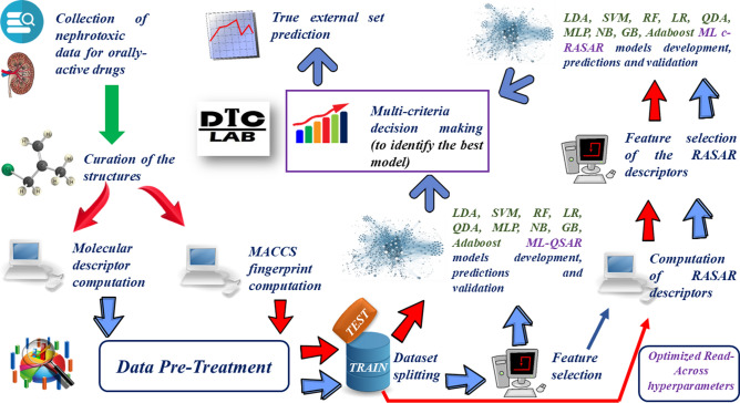
A detailed workflow has been presented in Fig. 1.

Fig. 1.

Detailed workflow of the model development procedure.

Results and discussion

Analysis of the chemical diversity of the dataset

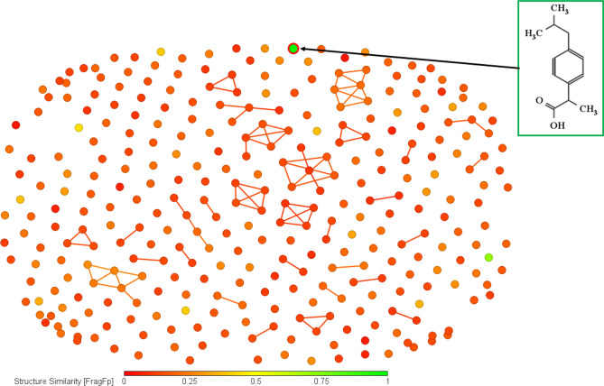
This initial level of analysis aimed to explore the structural diversity of the compounds constituting the dataset. Figure 2 represents a chemical diversity plot where the compounds are located according to their similarity. This plot was generated using DataWarrior (https://openmolecules.org/datawarrior/), using structural similarity information based on substructure fragment dictionary-based binary FragFp (Similarity limit: Automatic, Similarity on: Structure[FragFp]). Taking a well-known nephrotoxic compound Ibuprofen as the reference, it is evident from this plot that the dataset is highly diverse, offering a significant challenge for developing reliable mathematical models.

Fig. 2.

Chemical diversity analysis shows that the dataset compounds are highly dissimilar, taking Ibuprofen as the reference standard.

Selection of the important molecular descriptors for QSAR analysis

For the efficient selection of essential features, we identified the descriptors that have high discriminating power between the positive and the negative classes, using the most discriminating feature selection algorithm³⁹. The reason for adopting this feature selection technique is that it is independent of any particular modeling algorithm, thus enabling a fair comparison between the developed ML models. We used a Java-based tool MDF_Identifier-v1.0, available from https://sites.google.com/jadavpuruniversity.in/dtc-lab-software/home to identify the most discriminating features. We selected those features that have absolute mean difference values > 0.05. A list of 21 descriptors falls under this category and has been presented in Supplementary materials SI-1.

Selection of the important RASAR descriptors for c-RASAR analysis

The selection of the essential RASAR descriptors follows the same algorithm as the selection of the essential molecular descriptors for QSAR analysis. The RASAR descriptors with an absolute mean difference of > 0.11 were selected for modeling analysis. In the case of RASAR descriptors computed from the selected molecular descriptors, five fall under this category, while six RASAR descriptors calculated from the MACCS fingerprints fall under this category. The computed RASAR descriptors used to develop c-RASAR models are presented in Supplementary materials SI-1.

Results of the ML-based QSAR and c-RASAR models

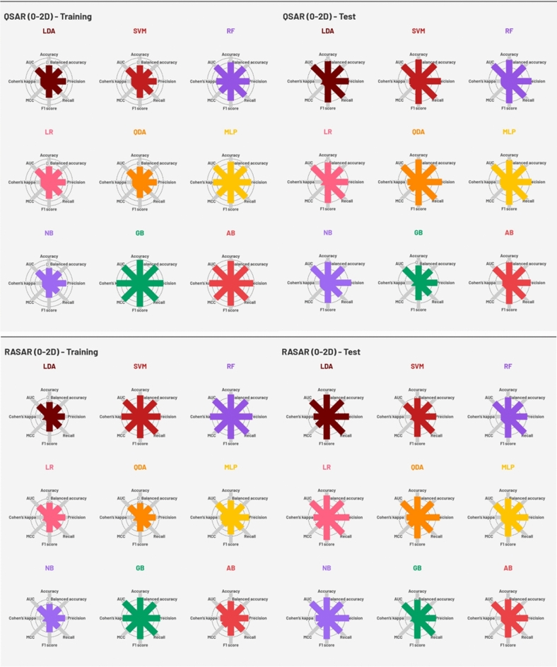
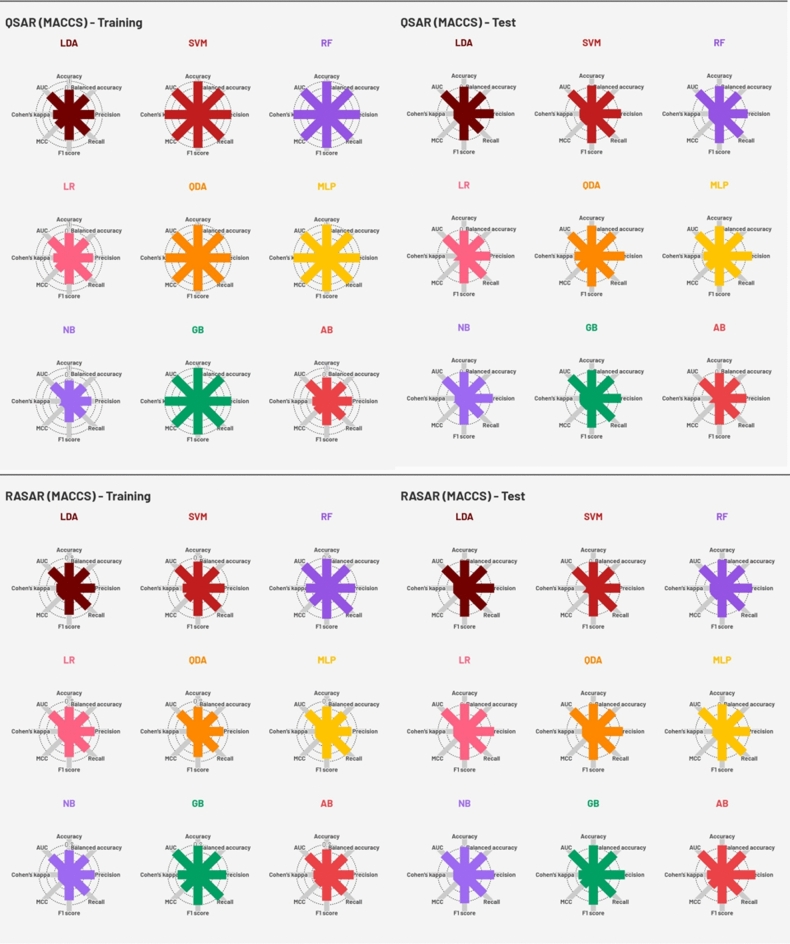
The quality metrics of all the developed QSAR models (nine using molecular descriptors and nine using MACCS fingerprints) and c-RASAR models (nine using the RASAR descriptors derived from the molecular features and nine using the RASAR descriptors derived from MACCS fingerprints) have been reported in Tables S1 and S2 in the Supplementary material SI-1, and also pictorially represented in Figs. 3 and 4. An array of different linear and non-linear ML modeling algorithms was adopted to generate classification-based QSAR models. The hyperparameters associated with the various models were optimized using GridSearchCV, adhering to a fivefold cross-validation strategy. The models’ quality was assessed using various classification-based validation metrics, and the best models were judged based on a “multi-criteria decision-making” strategy (to be discussed later in the manuscript).

Fig. 3.

Radar plots representing the performance metrics of the QSAR and c-RASAR models developed from 0-2D descriptors.

Fig. 4.

Radar plots representing the performance metrics of the QSAR and c-RASAR models developed from MACCS fingerprints.

This work applied a hybrid methodology of RASAR to predict the nephrotoxicity potential of drugs/drug candidates. This research aims to develop a predictive model that can be used for the virtual screening of a database of potential drugs. No specific receptor binding affinity or enzyme inhibition has been modeled here; the response modeled here is the binary data of nephrotoxicity potential. The multi-criteria decision-making considering training, cross-validation, and external set statistics clearly demonstrates that RASAR models perform better than traditional QSAR models reported in this work (vide infra).

Results for the cross-validation of all the developed models

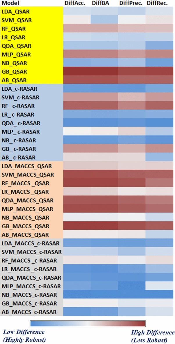
Cross-validation is an integral aspect to judge the robustness and stability of a model and to ensure that the overall quality of models is not dependent on a certain limited number of compounds only. The purpose of cross-validation is to check whether the performance of a model is stable even with the removal of certain data points from the training set. In the present investigation, we have cross-validated all our developed QSAR and c-RASAR models to check their robustness. We have performed rigorous cross-validation by adopting 20 times fivefold cross-validation strategy using Accuracy, Balanced Accuracy, Precision, and Recall as the objective functions. The results of cross-validation have been presented in Table S3 of the Supplementary material SI-1. From this table, it can be observed that there has been an increase in robustness (indicated by the marginal decrease in the cross-validated objective functions) of the c-RASAR models as compared to the conventional QSAR models, indicating that the models are not overfitted. Moreover, the significantly reduced number of modeling descriptors in the c-RASAR models provides greater compliance to the statistical considerations. Figure 5 presents a heat map of the absolute difference between the individual metric values and their cross-validated values. It can be clearly observed that the overall robustness of the MACCS QSAR models are lower, while the MACCS c-RASAR models are the most robust.

Fig. 5.

A heat map that pictorially demonstrates the robustness of the developed models after 20 times fivefold cross-validation. It is observed that MACCS c-RASAR models are highly robust. (DiffAcc = Absolute difference between Accuracy and AccuracyCV, DiffBA = Absolute difference between Balanced Accuracy and Balanced AccuracyCV, DiffPrec = Absolute difference between Precision and PrecisionCV, DiffRec = Absolute difference between Recall and RecallCV).

Identification of the best-performing model – An application of the Sum of Ranking Difference (SRD) approach

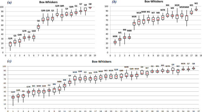
Since we have developed many mathematical models using different combinations of modeling descriptors, it is critical to identify the best-performing model directly. This is because this judgment should ideally encompass factors like robustness and predictivity. Therefore, we have adopted a multi-criteria decision-making strategy to judge the best-performing models using many objective functions. The Sum of Ranking Differences (SRD) is a well-known method to estimate the best-performing model based on multiple criteria³⁵. In this approach, the data should be arranged in a matrix with the metric values in the column and models in the rows. The metric values should be scaled (for example, scaled to unit length) column-wise, and then the scaled matrix may be transposed so the comparison models appear column-wise. Then, the absolute difference between the standard reference (which may be the maximum value row-wise) and individual method ranks is deduced and summed for each technique. In this manner, the sum of ranking difference (SRD) values is calculated for each method. An SRD value closer to zero (i.e., the closer the ranking is to the reference value) signifies that the model is better. Concerning external predictivity, we have considered metrics like Accuracy, Balanced Accuracy, Precision, Recall, F1_score, MCC, Ckappa, and AUC that define the predictive performance on the test set. Additionally, metrics like AccuracyCV, Balanced AccuracyCV, PrecisionCV, and RecallCV were considered for encoding information relating to robustness. Since the difference between a metric and its cross-validated value is a measure of robustness, we have additionally considered the absolute differences in the training set Accuracy, Balanced Accuracy, Precision, and Recall, with the AccuracyCV, Balanced AccuracyCV, PrecisionCV, and RecallCV, respectively. These 16 different parameters, representing robustness and predictivity of models, were considered for SRD analysis. We have validated the method using leave-one-seventh-out cross-validation. The scaled SRD values between 0 and 100 were calculated using the software named CRRN_DNA (downloaded from http://knight.kit.bme.hu/CRRN). The results were graphically analyzed by plotting the % SRD data (Fig. 6) for each modeling technique in a random environment, i.e., random ranking given to each data input for each model to generate all possible random sum of ranking differences. The SRD plot represents different modeling techniques placed in ascending order of their SRD values. The critical threshold XX1 indicates the region of randomness with p < 0.05 (i.e., probability of randomness less than 5%), Med means 50% randomness, and XX19 signifies 95% randomness.

Fig. 6.

SRD analysis of (a) the descriptor-based QSAR and c-RASAR models, (b) the fingerprint-based QSAR and c-RASAR models, and (c) all the developed models. The X-axis and left Y-axis represent the normalized SRD values, whose small values indicate better models. The right Y-axis represents the cumulative relative frequencies corresponding to the randomization test. (CRRN: Comparison of Ranks with Ranking Numbers).

Three different sets of analyses were performed. First, we intended to identify the best-performing ML models developed from molecular descriptors and their corresponding ML c-RASAR models. In the second case, we analyzed the ML QSAR models developed from the MACCS fingerprints and their corresponding ML c-RASAR models. Lastly, we took all the developed models and performed an overall comparison. As evident from Figs. 6a and 7a, where the analysis is between the descriptor-based ML QSAR models and their corresponding ML c-RASAR models, it can be observed that the overall performance of the ML c-RASAR models is better than the ML QSAR models. Additionally, the best-performing model appeared to be the LDA c-RASAR model. On the other hand, Figs. 6b and 7b represent the analysis between the fingerprint-based ML QSAR models and their corresponding ML c-RASAR models. Again, the c-RASAR models performed better than the corresponding QSAR models. The best-performing model in this comparison appeared to be the Adaboost MACCS c-RASAR model. The SRD analysis of all the developed models (36 models) has been presented in Figs. 6c and 7c. From this analysis comparing all the developed models, the LDA c-RASAR model appeared to be the best-performing model. This is quite significant where a linear model performs better than many other non-linear ML models, using different types of descriptors and fingerprints, thus demonstrating the potential of c-RASAR models fortifying previous similar observations^20,21,25,51. The models are represented in the following codes: Q1-Q9 = LDA, SVM, RF, LR, QDA, MLP, NB, GB, and AB QSAR models developed from molecular descriptors, M1-M9 = LDA, SVM, RF, LR, QDA, MLP, NB, GB, and AB QSAR models developed from MACCS fingerprints, Q1R-Q9R = LDA, SVM, RF, LR, QDA, MLP, NB, GB and AB c-RASAR models developed from molecular descriptors and M1R-M9R = LDA, SVM, RF, LR, QDA, MLP, NB, GB and AB c-RASAR models developed from MACCS fingerprints.

Fig. 7.

Leave-1/7^th-out cross-validated SRD results showing that the LDA q-RASAR model (Q1R) is the best model. The X-axis represents the models and the Y-axis are the corresponding Leave-1/7^th-out cross-validated SRD.

Interpretation of the RASAR descriptors used to develop the LDA c-RASAR model

One of the essential purposes of any modeling analysis is to interpret the modeled features and provide an idea of their contribution toward the endpoint of interest. After selecting the best-performing model (LDA c-RASAR) by statistical evaluation using the SRD approach, we used the LDA coefficients to identify the contribution of the RASAR descriptors toward the model. Since the c-RASAR models are developed using similarity and error-based RASAR descriptors, it is essential to note that the interpretation is relative, and it considers the structural characteristics of the close source congeners. The descriptor RA function is a read-across-derived function, which is a compact representation of the entire structural and physicochemical descriptor space into a single variable⁵². Since it encodes all chemical information, this descriptor contributes positively to the response. This can be observed in the case of Dabrafenib (283), which has a high value of RA function and is nephrotoxic. Similarly, Ribavirin (265) has a very low value of RA function and is observed to be non-nephrotoxic. The descriptor CVsim demonstrates the coefficient of variation of the similarity values of close source congeners for a particular target compound, and this descriptor contributes positively towards the response. This indicates the high dispersion of the similarity values of the close congeners, inferring that the dataset is highly diverse, as also previously demonstrated in Fig. 2. This can be exemplified by Irbesartan (197), that have a high value of CVsim and is an active compound, while inactive compounds like Chlorzoxazone (50) have a lower CVsim value. The descriptor MaxNeg is the similarity value to the closest negative/inactive source compound for an individual query compound, and this descriptor contributes negatively to the response. A query compound having a higher value of MaxNeg justifies that it shares a high similarity to an inactive/negative compound, which increases the propensity of the query compound to be inactive. On the other hand, a compound having a lower maximum similarity to a negative compound is most likely to become an active compound. This can be exemplified with the inactive compound Theophylline (261), which has a high value of MaxNeg, while active compounds like Cefpodoxime (167) have a lower value of MaxNeg. This is shown pictorially in Fig. 8 where we also analyze the structures of the close source compounds. It is observed that the nearest inactive neighbor of Theophylline (an inactive compound) is Caffeine, which is highly similar in structure. However, the nearest inactive neighbor of Cefpodoxime (an active compound) is Terazosin, with a very low level of similarity. This proves that the highly similar compounds of Cefpodoxime are active, explaining why the MaxNeg expresses a negative contribution. The descriptor s_m¹, a.k.a. the Banerjee-Roy similarity coefficient, is a novel concordance measure that helps identify activity cliffs²¹. However, from a modeling point of view, this descriptor makes a positive contribution. As evident from the formula mentioned in the work of Banerjee and Roy²¹, a positive contribution is expected since a higher value of MaxPos than MaxNeg signifies that the query compound has a propensity to become active. This can be exemplified with active compounds like Valsartan (11), which has a high value of s_m¹. Similarly, inactive compounds like Labetalol (142) have lower values of s_m¹. The descriptor g_m_class is a modified version of the Banerjee-Roy concordance coefficient, and this descriptor contributes positively to the response. The main property of this descriptor is that it is binary (values are either 0 or 1), and can potentially identify the propensity of a particular compound to be active or inactive. This can be observed in active compounds like Rabeprazole (102) that has a high value of g_m_class, while inactive compounds like Riboflavin (152) have a lower value of g_m_class.

Fig. 8.

Analysis of the nearest negative/inactive compounds for active and inactive query compounds.

Predictions of the true external set data using the LDA c-RASAR model

This is an essential aspect that further justifies the generalizability of the developed model. We identified 111 compounds labeled as nephrotoxic from the DrugBankDB. It should be noted that these 111 compounds were exclusively the compounds not present in the training set and are not organometallic. However, analyzing the predictive performance revealed that out of the 111 data points, 73 compounds were correctly identified as nephrotoxic, which corresponds to a sensitivity value of 0.658. Thus, it can be concluded that the LDA c-RASAR model also generalizes well with true external data and efficiently identifies nephrotoxic compounds. The prediction results are presented in Supplementary Materials SI-1.

t-SNE analysis of the descriptor and fingerprint spaces

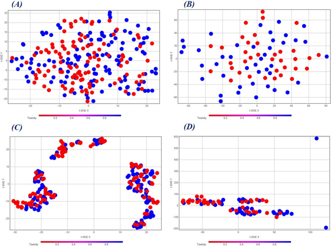
This analysis reflects not only the diversity of the dataset but also how the individual descriptor and fingerprint spaces encode the chemical information. This is analyzed by adopting non-linear dimensionality reduction techniques like the t-SNE³⁸. We have subjected our different training and test sets individually encoded by different feature matrices to generate the t-SNE plots using the DataWarrior software (https://openmolecules.org/datawarrior/). Fig. 9 represents the t-SNE plots derived from the molecular descriptors of the training and test sets that were used for QSAR modeling (Figs. 9(A) and 9(B)) and the corresponding similarity and error-based RASAR descriptors that were used for c-RASAR modeling (Figs. 9(C) and 9(D)). From the visual representation, one can easily understand how well the RASAR descriptors encode chemical information, reflected in the tight clustering of the data points in Figs. 9(C) and 9(D). This highlights the underlying reasons why most of the c-RASAR models had a superior ranking in the SRD analysis, which is a reflection of the robustness and external predictivity of the models.

Fig. 9.

t-SNE plots of the (A) Training set data using the selected molecular descriptors, (B) Test set data using the selected molecular descriptors, (C) Training set data using the corresponding RASAR descriptors developed from descriptor-based feature space, and (D) Test set data using the corresponding RASAR descriptors developed from descriptor-based feature space. These plots highlight how well the RASAR descriptors encapsulate the complete chemical information, as evident from the tight clustering.

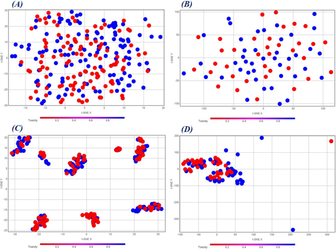
On the other hand, Fig. 10 represents the t-SNE plots of the training and test sets of the MACCS fingerprints that were used for QSAR modeling (Figs. 10(A) and 10(B)) and the corresponding similarity and error-based RASAR descriptors that were used for c-RASAR modeling (Figs. 10(C) and 10(D)). Similar to the previous case, the c-RASAR descriptors computed from MACCS fingerprints were observed to encode chemical information very efficiently, and one can observe from Fig. 10C how it produces a near-ideal level of clustering of data points in the training set. This is also justified since, in Fig. 5, it is observed that the MACCS c-RASAR models are the most robust among all the other approaches. Additionally, better clustering is observed in the test set constituting the RASAR descriptors compared to the MACCS fingerprints. Another important point to note is that in all the cases in this current study, the c-RASAR models are developed using only a few modeling descriptors that further justify their potential and statistical reliability.

Fig. 10.

t-SNE plots of the (A) Training set data using the MACCS fingerprints, (B) Test set data using the MACCS fingerprints, (C) Training set data using the corresponding RASAR descriptors developed from fingerprint-based feature space, and (D) Test set data using the corresponding RASAR descriptors developed from fingerprint-based feature space. Like Fig. 9, these plots also highlight how well the RASAR descriptors encapsulate the complete chemical information, as evident from the tight clustering.

Analysis of the activity cliffs using a supervised algorithm for dimensionality reduction

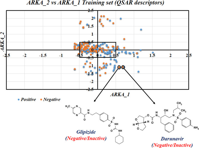
We discussed above how the RASAR descriptors efficiently encode the chemical information through t-SNE analysis. However, one typical drawback of this approach is its unsupervised nature, which does not allow for the identification of potential activity cliffs. Therefore, we have adopted a supervised dimensionality reduction technique – the ARKA framework for identifying activity cliffs ¹⁵. The Arithmetic Residuals in k-groups Analysis (ARKA) is a recently developed supervised dimensionality reduction technique proposed by Banerjee and Roy ¹⁵. The basic theory behind this approach is that the information of descriptors (in the normalized form of 0–1) having a mean value greater in the active/toxic class as compared to the inactive/non-toxic class (signifying positive mean difference values), gets incorporated into ARKA_1, while the descriptors obeying the opposite trend is incorporated into ARKA_2, with suitable weights in both the cases, based on the magnitude of mean differences. This analysis is done on the training set descriptor matrix to identify the two classes of descriptors, and a weighted function on the standardized descriptor matrices is applied to compute the ARKA descriptors for the training and test sets. As per this theory, the positive/toxic compounds should have a positive ARKA_1 and negative ARKA_2 value, which is opposite in the case of inactive compounds. If, by chance, a positive data point has negative ARKA_1 and positive ARKA_2, or a negative data point has a positive ARKA_1 and a negative ARKA_2, then such compounds can be considered as activity cliffs, provided that we consider ARKA values greater than ± 0.5. In the current investigation, we have computed the ARKA descriptors, using the tool ARKAdesc-v2.0 available from https://sites.google.com/jadavpuruniversity.in/dtc-lab-software/arithmetic-residuals-in-k-groups-analysis-arka, for the training set that has been defined using the selected 21 molecular descriptors employed for QSAR analysis, and an ARKA_2 (Y-axis) v/s ARKA_1 (X-axis) scatter plot was developed. Many less confident data points (points in the first and third quadrants) and two distinct activity cliffs (both in the fourth quadrant) were identified. More significant activity cliffs may be determined based on their distance from the origin (which is equivalent to the square root of the sum of the ARKA descriptors), provided positive compounds are located in the second quadrant and negative compounds are located in the fourth quadrant. Additionally, many data points were in the less modelable region (the central rectangle surrounding the origin) and the borderline zone (± 0.5 on either side of the axes). The corresponding ARKA_2 vs ARKA_1 plot has been shown in Fig. 11. More theoretical information on the ARKA framework can be found in the work of Banerjee and Roy ¹⁵.

Fig. 11.

ARKA_2 vs ARKA_1 plot for the training set defined by molecular descriptors. Activity cliffs like Glipizide and Darunavir were identified.

The compound Glipizide, identified as an activity cliff, was reported as non-nephrotoxic. Let’s analyze the Gaussian Kernel similarity of this compound with some of its close source congeners (as identified by the Read-Across algorithm of the RASAR descriptor calculator tool). All the similarity levels are very low. Moreover, out of the ten closest source neighbors of Glipizide, eight were in the nephrotoxic class, and only two were in the non-nephrotoxic class, suggesting that this compound has more structural similarity with the nephrotoxic compounds. This explains why Glipizide has been identified as an activity cliff. Darunavir, an antiretroviral drug, has also been identified as an activity cliff from the ARKA analysis. This drug was also labeled as a non-nephrotoxic compound, but all its closest ten nearest neighbors belong to the nephrotoxic class of drugs, which again suggests that this drug has more structural similarity to a nephrotoxic compound. If we observe the predictions from the QDA QSAR model (the best performing QSAR model developed from molecular descriptors), both the compounds have been mispredicted as nephrotoxic compounds, thus implying their activity cliff nature.

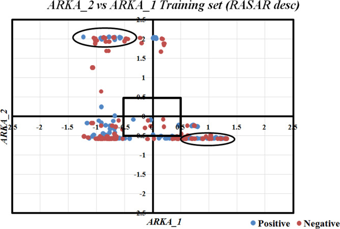
So far, the analysis and identification of the activity cliffs have centered on the molecular descriptors employed in QSAR modeling. However, as previously stated in the manuscript and also in ^53–55, the RASAR descriptors encode the chemical information more efficiently, ultimately reducing the number of modeling descriptors. We have computed the ARKA descriptors on the selected 5 RASAR descriptors used to develop the c-RASAR models to explore and identify additional activity cliffs, which the standard molecular descriptors could not identify. It can be observed from the ARKA_2 vs ARKA_1 plot of the training set (Fig. 12) that a lower number of data points existed inside the central rectangular zone (as compared to Fig. 11) ultimately infers that the modelability of the dataset has been increased on the application of the RASAR descriptors. Additionally, this plot identifies many activity cliffs (including the previously identified Glipizide and Darunavir) that belong to both the active/positive and inactive/negative classes. The regions enclosed by the two ellipses demonstrate the location of these activity cliffs.

Fig. 12.

ARKA_2 vs ARKA_1 plot for the training set defined by the RASAR descriptors. The ellipses represent the location of the multiple activity cliffs. It is to be noted that a minimal number of compounds exist in the central rectangular region, inferring the enhancement of the modelability of the application of the RASAR descriptors.

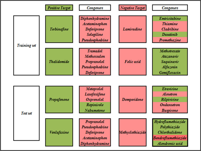
In this case, we analyzed the two most significant activity cliffs from each positive and negative class. Initially, we have identified the compounds in the opposite quadrant (i.e., positive compounds in the second quadrant and negative compounds in the fourth quadrant). Among these compounds, we have computed the Euclidean Distance from the origin using the formula mentioned in Eq. 1. We have identified four compounds (two each) with the highest Euclidean Distance values from the positive and negative classes, justifying that these compounds are “most confident activity cliffs”. Additionally, we have explored the five nearest neighbors from our RASAR analysis and observed that most of these close congeners are from the opposite class of activity. This is pictorially represented in Fig. 13, where we analyze the activity cliffs from the training and test sets.

1

Fig. 13.

Activity cliffs from the positive and negative classes and their five closest neighbors. The green color indicates active/positive compounds, while the red indicates inactive/negative compounds.

ED is the Euclidean Distance, X is the value of ARKA_1, and Y is the value of ARKA_2. The confidence in the activity cliff nature of a compound should increase with its location from the origin, i.e., with an increase in the value of ED, provided it is located in the wrong quadrant, as mentioned above.

Activity cliffs like Terbinafine (Positive), Thalidomide (Positive), Folic acid (Negative), and Venlafaxine (Positive) have all of their five closest neighbors in the opposite class. This infers that these compounds have structural similarities towards their opposite class, which eventually hinders the modelability of the dataset. If we consider the predictions of these compounds by our LDA c-RASAR model, it can be observed that all these compounds have been mispredicted into their opposite class. In the case of compounds like Propafenone (Positive) and Methyclothiazide (Negative), although compounds of the same class exist in the list of closest congeners, it can be observed that a higher fraction of the closest congeners belongs to the opposite class. If we consider their predictions, it was observed that Propafenone was mispredicted as inactive, while Methyclothiazide was mispredicted as active. However, in the cases of Lamivudine (Negative) and Domperidone (Negative), although a higher fraction of the closest source congeners belongs to the same class, it can be observed that the similarity levels to the closest neighbor are high but drastically decreases afterward. This infers that only one compound is close to the target compounds (Lamivudine and Domperidone). In contrast, the other close congeners are located quite far away in terms of their similarities. Therefore, the closest neighbor is the one that describes the propensity of the target compounds towards being active or inactive. If we analyze the closest neighbors of Lamivudine, it has a high similarity value of 0.971 with Emtricitabine, while the similarity level with its second closest compound (Thiamine) is 0.00002. A similar observation was obtained from Domperidone with a similarity level of 0.069 with the closest neighbor Etravirine, while the similarity level with the second closest compound (Alosetron) is only 0.001. As both Emtricitabine (Positive) and Etravirine (Positive) belong to the opposite class of Lamivudine and Domperidone, respectively, it can be concluded that this leads to the mis-prediction of both the compounds by our LDA c-RASAR model.

Comparison with the previous works

Gong et al. ³¹ and Shi et al. ³² developed multiple machine-learning models to predict the nephrotoxicity of compounds. However, the works of Connor et al. ³⁴ involved compilation of the data from the two sources and curation adhering to the strategy proposed by Tropsha’s group ³⁶. These authors mapped the molecules to the DrugBank database to identify the drug molecules and further verified with the Anatomical, Therapeutic and Chemical (ATC) index ^56,57 to identify “orally administered drugs” with nephrotoxicity data. These nephrotoxicity data from the two literature sources were cross-checked with sources like the FDA and DrugBankDB to obtain a final list of experimental data. This particular step was crucial since it can be observed from the works of Connor et al. that many molecules had contrasting nephrotoxicity labels in the two different sources (Gong et al. and Shi et al.). In this regard, our model stands out since we have used the fully curated dataset presented by Connor et al. to develop Machine Learning models. This increased reliability of the modeling data used, ultimately increasing the acceptability of our model and its predictions. A detailed comparison report of our work with the works of Gong et al. and Shi et al. has been presented in Table 1, which justifies how this present study is better. Sun et al. ³³ also predicted the nephrotoxicity of natural products and drugs. Although not specific for orally active drugs, the poor external validation results showing MCC values of 0.000 and 0.089 of the ANN and SVM models respectively justify that the models did not generalize well with the test set data. This is not the case of our LDA c-RASAR model, as its external predictivity is quite good where MCC value is 0.431. Therefore, we can infer that our LDA c-RASAR model is superior in terms of reliability and prediction quality to predict the nephrotoxicity of orally administered drugs.

Table 1.

Comparison of our work with the works of Gong et al. and Shi et al.

Parameters	Gong et al. 31	Shi et al. 32	Our work
Dataset strictly focusing on drug molecules (more specifically, orally active drug molecules)	No	No	Yes
True external set prediction	Yes	No	Yes
Size of the true external set	Lower (n = 71)	-	Higher (n = 111)
Activity cliffs analysis	No	No	Yes
Statistical tests (using multi-criteria decision-making approaches) for the identification of best models	No	No	Yes (by using the Sum of Ranking Differences approach)
The presence of conflicting data labels for the same compounds reduces the reliability of the models	Yes (e.g., Aspirin has been labelled as Nephrotoxic)	Yes (e.g., Aspirin has been labelled as Non-nephrotoxic)	No, since we developed models on the curated dataset presented by Connor et al
Rigorous cross-validation	Yes	Yes	Yes

Conclusion

Drug-induced nephrotoxicity is an area of concern since our kidneys are associated with the removal of toxic substances and metabolites from the blood. A lot of drugs that we take orally for treating specific ailments are often silently associated with producing nephrotoxicity. Since experimental identification is tedious and involves ethical complications, we have developed Machine Learning (ML) models to easily screen drugs, identifying their potential nephrotoxicity when administered orally. We have used a highly curated data set of orally active drugs for the reliability of the developed models. Simple and interpretable 0-2D molecular descriptors and MACCS fingerprints were used to develop ML models. We have also developed ML c-RASAR models on the feature spaces encoded by the selected 0-2D descriptors and MACCS fingerprints to incorporate similarity-based considerations. This resulted in the enhancement of robustness and predictivity of the c-RASAR models, justifying the more efficient and concise use of the chemical information of the close source neighbors. All the developed QSAR and c-RASAR models were subjected to statistical comparison using the Sum of Ranking Differences (SRD) approach, considering factors associated with robustness and external predictivity. This analysis suggested that the LDA c-RASAR model, developed from the feature space of the molecular descriptors, was the best-performing model among 36 different linear and non-linear ML models. Once again, this infers the successful incorporation of the non-linear information into a linear modeling framework by the RASAR descriptors, which results in linear models having enhanced performance than non-linear models.

RASAR is sufficiently different from conventional QSAR in its algorithm. In case of QSAR, the division of the data set into training and test sets is done after computation of descriptors while RASAR descriptors are computed after division of the data set intro training and test sets. The RASAR descriptors are computed based on a similarity concept and those from the training set are computed from training set molecules only using the leave-same-out approach. This is unique in RASAR thus contributing sufficient novelty to the approach. In this particular work, we showed that this algorithm can also successfully be used in case of feature spaces defined by fingerprints, while the previous works dealt with c-RASAR modeling on topological descriptor space. The results of the current study showed that the MACCS c-RASAR models appeared to be among the most robust models, while the LDA c-RASAR model developed from topological descriptors had an overall best performance, making it the most robust and highly predictive one. In this study, we showed the limitations of the previously reported nephrotoxicity models in the comparison section of our manuscript, and evidently, the previous models suffered from reliable experimental data on which the models were developed, and suffered ambiguity in the data labels. In our study, we have used a fully curated set of nephrotoxicity data presented by Weida Tong and co-workers ³⁴ that encourage the use of NAMs to develop machine learning models, thereby enhancing the reliability and acceptability of our models.

To assess the model performance on true external set data, we have used the LDA c-RASAR model to predict the nephrotoxicity of the approved drugs from the DrugBankDB. The successful results on the true external set justify the reliability of our simple model. This LDA c-RASAR model can thus be used for quick and efficient nephrotoxicity prediction for orally active drugs. The efficient identification of activity cliffs by the ARKA analysis and the tight and distinct clustering observed in the t-SNE plots exactly points out the true potential of the c-RASAR approach in not only optimizing the utilization of the feature space but also in the identification of activity and prediction cliffs. This study opens up the avenue for successfully incorporating the similarity considerations that can be used to optimize the utilization of the available feature space, resulting in enhanced predictivity. This is particularly useful in the phase of drug discovery and development where a more accurate prioritization of chemicals is desired, leading to optimization of the existing molecules to lower their toxicity profiles while retaining or enhancing their therapeutic effects. Considering the increasing uses of deep learning in cheminformatics ⁵⁸, it would also be interesting to see the prediction performance of the c-RASAR approach when subjected to a deep learning modelling framework, thus paving the way for future research.

Author contributions

Arkaprava Banerjee: Data curation, Formal analysis, validation, software, Writing—Initial draft Kunal Roy: Conceptualization, Funding acquisition, Supervision, Writing—Editing.

Funding

This research has been funded by the Life Sciences Research Board, DRDO, New Delhi (LSRB/01/15001/M/LSRB-394/SH&DD/2022). Financial assistance from SERB, New Delhi is also thankfully acknowledged.

Data availability

The source data used to develop the models reported in this paper are available in the Supplementary Materials SI-1. The RASAR descriptors and their significance has been tabulated in Supplementary Material SI-2 The software tools used for the Read-Across predictions and the computation of the RASAR descriptors and ARKA descriptors are freely available from https://sites.google.com/jadavpuruniversity.in/dtc-lab-software/home and https://sites.google.com/jadavpuruniversity.in/dtc-lab-software/arithmetic-residuals-in-k-groups-analysis-arka

Declarations

A preprint version of the article has been deposited to ChemRxiv (https://doi.org/10.26434/chemrxiv-2024-57klw). Kunal Roy: Conceptualization, Funding acquisition, Supervision, Writing—Editing.

Competing interests

The authors declare no competing interests.

Supplementary Information

The online version contains supplementary material available at 10.1038/s41598-024-85063-y.

References

- 1.Vleet, T. R. V. & Schnellmann, R. G. Toxic nephropathy: environmental chemicals. Sem. Nephro.23, 500–508 (2003). [DOI] [PubMed] [Google Scholar]
- 2.Kellum, J. A. et al. Acute kidney injury. Nat. Rev. Dis. Primers.7, 52 (2021). [DOI] [PubMed] [Google Scholar]
- 3.Kulkarni, P. Prediction of drug-induced kidney injury in drug discovery. Drug Metabol. Rev.53, 234–244 (2021). [DOI] [PubMed] [Google Scholar]
- 4.Redfern, W. S. et al. Impact and frequency of different toxicities throughout the pharmaceutical life cycle. Toxicologist.114, 231 (2010). [Google Scholar]
- 5.Choudhury, D. & Ahmed, Z. Drug-associated renal dysfunction and injury. Nat. Clin. Pract. Nephrol.2, 80–91 (2006). [DOI] [PubMed] [Google Scholar]
- 6.Gai, Z., Gui, T., Kullak-Ublick, G. A., Li, Y. & Visentin, M. The role of mitochondria in drug-induced kidney injury. Front. Physiol.11, 1079 (2020). [DOI] [PMC free article] [PubMed] [Google Scholar]
- 7.Simon, N., Morin, C., Urien, S., Tillement, J. P. & Bruguerolle, B. Tacrolimus and sirolimus decrease oxidative phosphorylation of isolated rat kidney mitochondria. Br. J. Pharmacol.138, 369–376 (2003). [DOI] [PMC free article] [PubMed] [Google Scholar]
- 8.Sawyer, M. H., Webb, D. E., Balow, J. E. & Straus, S. E. Acyclovir-induced renal failure: Clinical course and histology. Amer. J. Med.84, 1067–1071 (1988). [DOI] [PubMed] [Google Scholar]
- 9.Min, S.-Y., Ha, D.-S. & Ha, T.-S. Puromycin aminonucleoside triggers apoptosis in podocytes by inducing endoplasmic reticulum stress. Kidney Res Clin Prac.37, 210–221 (2018). [DOI] [PMC free article] [PubMed] [Google Scholar]
- 10.Roy, K., Kar, S. & Das, R. N. Understanding the basics of QSAR for applications in pharmaceutical sciences and risk assessment (Academic Press, 2015). [Google Scholar]
- 11.Brogi, S., Ramalho, T. C., Kuca, K., Medina-Franco, J. L. & Valko, M. Editorial: in silico methods for drug design and discovery. Front. Chem.8, 612 (2020). [DOI] [PMC free article] [PubMed] [Google Scholar]
- 12.Hansch, C., Hoekman, D. & Gao, H. Comparative QSAR: Toward a deeper understanding of chemicobiological interactions. Chem. Rev.96, 1045–1076 (1996). [DOI] [PubMed] [Google Scholar]
- 13.Gini, G. QSAR methods. In In Silico Methods for Predicting Drug Toxicity (ed. Benfenati, E.) (Springer NY, 2022). [Google Scholar]
- 14.Hessler, G. & Baringhaus, K. H. Artificial intelligence in drug design. Molecules23, 2520 (2018). [DOI] [PMC free article] [PubMed] [Google Scholar]
- 15.Banerjee, A. & Roy, K. ARKA: a framework of dimensionality reduction for machine-learning classification modeling risk assessment and data gap-filling of sparse environmental toxicity data. Environ. Sci. Process. Impacts26(6), 991–1007 (2024). [DOI] [PubMed] [Google Scholar]
- 16.Gajewicz, A. What if the number of nanotoxicity data is too small for developing predictive Nano-QSAR models? An alternative read-across based approach for filling data gaps. Nanoscale9, 8435–8448 (2017). [DOI] [PubMed] [Google Scholar]
- 17.Chatterjee, M., Banerjee, A., De, P., Gajewicz-Skretna, A. & Roy, K. A. novel quantitative read-across tool designed purposefully to fill the existing gaps in nanosafety data. Environ. Sci. Nano.9(1), 189–203 (2022). [Google Scholar]
- 18.Manganelli, S. & Benfenati, E. Use of Read-Across tools. In In Silico Methods for Predicting Drug Toxicity (ed. Benfenati, E.) (Springer NY, 2016). [Google Scholar]
- 19.Banerjee, A. & Roy, K. First report of q-RASAR modeling toward an approach of easy interpretability and efficient transferability. Mol. Divers.26, 2847–2862 (2022). [DOI] [PubMed] [Google Scholar]
- 20.Banerjee, A. & Roy, K. On Some novel similarity-based functions used in the ML-based q-RASAR approach for efficient quantitative predictions of selected toxicity end points. Chem. Res. Toxicol.36, 446–464 (2023). [DOI] [PubMed] [Google Scholar]
- 21.Banerjee, A. & Roy, K. Prediction-inspired intelligent training for the development of classification read-across structure–activity relationship (c-RASAR) models for organic skin sensitizers: assessment of classification error rate from novel similarity coefficients. Chem. Res. Toxicol.36, 1518–1531 (2023). [DOI] [PubMed] [Google Scholar]
- 22.Banerjee, A. & Roy, K. Read-across-based intelligent learning: development of a global q-RASAR model for the efficient quantitative predictions of skin sensitization potential of diverse organic chemicals. Environ. Sci. Process. Impacts25, 1626–1644 (2023). [DOI] [PubMed] [Google Scholar]
- 23.Wang, Y. et al. From molecular descriptors to the developmental toxicity prediction of pesticides/veterinary drugs/bio-pesticides against zebrafish embryo: Dual computational toxicological approaches for prioritization. J. Hazard. Mater.476, 134945 (2024). [DOI] [PubMed] [Google Scholar]
- 24.Jiang, J., Cai, W., Chen, Z., Liao, X. & Cai, Z. Prediction of acute toxicity for Chlorella vulgaris caused by tire wear particle-derived compounds using quantitative structure-activity relationship models. Water Res.256, 121643 (2024). [DOI] [PubMed] [Google Scholar]
- 25.Kumar, V., Banerjee, A. & Roy, K. Breaking the barriers: Machine-learning-based c-RASAR approach for accurate blood–brain barrier permeability prediction. J. Chem. Inf. Model.64, 4298–4309 (2024). [DOI] [PubMed] [Google Scholar]
- 26.Pandey, S. K. & Roy, K. Development of a read-across-derived classification model for the predictions of mutagenicity data and its comparison with traditional QSAR models and expert systems. Toxicology500, 153676 (2023). [DOI] [PubMed] [Google Scholar]
- 27.Banerjee, A., De, P., Kumar, V., Kar, S. & Roy, K. Quick and efficient quantitative predictions of androgen receptor binding affinity for screening Endocrine Disruptor Chemicals using 2D-QSAR and Chemical Read-Across. Chemosphere309, 136579 (2022). [DOI] [PubMed] [Google Scholar]
- 28.Banerjee, A. & Roy, K. Machine-learning-based similarity meets traditional QSAR: “q-RASAR” for the enhancement of the external predictivity and detection of prediction confidence outliers in an hERG toxicity dataset. Chemom. Intell. Lab. Syst.237, 104829 (2023). [Google Scholar]
- 29.Varsou, D.-D. et al. The Round Robin approach applied to nanoinformatics: Consensus prediction of nanomaterials zeta potential. Beilstein J. Nanotechnol. 15, 1536–1553 (2024) [DOI] [PMC free article] [PubMed] [Google Scholar]
- 30.Banerjee, A. & Roy, K. How to correctly develop q-RASAR models for predictive cheminformatics. Expert Opin. Drug Discov.19, 1017–1022 (2024). [DOI] [PubMed] [Google Scholar]
- 31.Gong, Y. et al. In silico prediction of potential drug-induced nephrotoxicity with machine learning methods. J. Appl. Toxicol.42, 1639–1650 (2022). [DOI] [PubMed] [Google Scholar]
- 32.Shi, Y., Hua, Y., Wang, B., Zhang, R. & Li, X. In silico prediction and insights into the structural basis of drug induced nephrotoxicity. Front. Pharmacol.12, 793332 (2022). [DOI] [PMC free article] [PubMed] [Google Scholar]
- 33.Sun, Y., Shi, S., Li, Y. & Wang, Q. Development of quantitative structure-activity relationship models to predict potential nephrotoxic ingredients in traditional Chinese medicines. Food Chem. Toxicol.128, 163–170 (2019). [DOI] [PubMed] [Google Scholar]
- 34.Connor, S., Li, T., Qu, Y., Roberts, R. A. & Tong, W. Generation of a drug-induced renal injury list to facilitate the development of new approach methodologies for nephrotoxicity. Drug Discov. Today29, 103938 (2024). [DOI] [PubMed] [Google Scholar]
- 35.Racz, A., Bajusz, D. & Heberger, K. Multi-Level comparison of machine learning classifiers and their performance metrics. Molecules24, 2811 (2019). [DOI] [PMC free article] [PubMed] [Google Scholar]
- 36.Fourches, D., Muratov, E. & Tropsha, A. Trust, But Verify: On the importance of chemical structure curation in cheminformatics and QSAR modeling research. J. Chem. Inf. Model.50, 1189–1204 (2010). [DOI] [PMC free article] [PubMed] [Google Scholar]
- 37.Mauri, A. alvaDesc: A Tool to Calculate and Analyze Molecular Descriptors and Fingerprints. In Ecotoxicological QSARs (ed. Roy, K.) (Springer NY, 2020). [Google Scholar]
- 38.van der Maaten, L. & Hinton, G. Visualizing data using t-SNE. J. Mach. Learn. Res.9, 2579–2605 (2008). [Google Scholar]
- 39.Murcia-Soler, M. et al. Artificial neural networks and linear discriminant analysis: A valuable combination in the selection of new antibacterial compounds. J. Chem. Inf. Comput. Sci.44, 1031–1041 (2004). [DOI] [PubMed] [Google Scholar]
- 40.Xanthopoulos, P., Pardalos, P.M., & Trafalis, T.B. Linear Discriminant Analysis. In Robust Data Mining. SpringerBriefs in Optimization. (Springer, New York, NY, 2013).
- 41.Lau, K. W. & Wu, Q. H. Online training of support vector classifier. Patt. Recog.36, 1913–1920 (2003). [Google Scholar]
- 42.Breiman, L. Random forests. Mach. Learn.45, 5–32 (2001). [Google Scholar]
- 43.Stoltzfus, J. C. Logistic regression: A brief primer. Aca. Emer. Med.18, 1099–1104 (2011). [DOI] [PubMed] [Google Scholar]
- 44.Srivastava, S., Gupta, M. R. & Frigyik, B. A. Bayesian quadratic discriminant analysis. J. Mach. Learn. Res.8, 1277–1305 (2007). [Google Scholar]
- 45.Chaudhuri, B. B. & Bhattacharya, U. Efficient training and improved performance of multilayer perceptron in pattern classification. Neurocomputing34, 11–27 (2000). [Google Scholar]
- 46.Ontivero-Ortega, M., Lage-Castellanos, A., Valente, G., Goebel, R. & Valdes-Sosa, M. Fast Gaussian Naïve Bayes for searchlight classification analysis. NeuroImage163, 471–479 (2017). [DOI] [PubMed] [Google Scholar]
- 47.Natekin, A. & Knoll, A. Gradient boosting machines, a tutorial. Front. Neurorobot.7, 21 (2013). [DOI] [PMC free article] [PubMed] [Google Scholar]
- 48.Wang, R. AdaBoost for feature selection, classification and its relation with SVM, a review. Phys. Procedia25, 800–807 (2012). [Google Scholar]
- 49.Snedecor, G. W. & Cochran, W. G. Statistical Methods 8th edn. (Wiley-Blackwell, 1989). [Google Scholar]
- 50.Fushiki, T. Estimation of prediction error by using K-fold cross-validation. Stat. Comput.21, 137–146 (2011). [Google Scholar]
- 51.Pandey, S. K., Banerjee, A. & Roy, K. Machine learning-based q-RASPR predictions of detonation heat for nitrogen-containing compounds. Mater. Adv.4, 5797–5807 (2023). [Google Scholar]
- 52.Banerjee, A., Kar, S., Pore, S. & Roy, K. Efficient predictions of cytotoxicity of TiO2-based multi-component nanoparticles using a machine learning-based q-RASAR approach. Nanotoxicology17, 78–93 (2023). [DOI] [PubMed] [Google Scholar]
- 53.Roy, K. & Banerjee, A. q-RASAR. A Path to Predictive Cheminformatics (Springer, 2024). [DOI] [PubMed] [Google Scholar]
- 54.Banerjee, A. et al. Molecular similarity in chemical informatics and predictive toxicity modeling: from quantitative read-across (q-RA) to quantitative read-across structure–activity relationship (q-RASAR) with the application of machine learning. Crit. Rev. Toxicol.54, 659–684 (2024). [DOI] [PMC free article] [PubMed] [Google Scholar]
- 55.Banerjee, A. & Roy, K. The application of chemical similarity measures in an unconventional modeling framework c-RASAR along with dimensionality reduction techniques to a representative hepatotoxicity dataset. Sci. Rep.14, 20812 (2024). [DOI] [PMC free article] [PubMed] [Google Scholar]
- 56.World Health Organization (WHO) Anatomical therapeutic chemical (ATC) classification index with defined daily doses (DDDs). Oslo: WHO Collaborating Centre for Drug Statistics Methodology. 2000:20.
- 57.World Health Organization (WHO) collaborating centre for drug statistics methodology. Guidelines for ATC classification and DDD assignment. Norwegian Institute of Public Health; 2021. 2022.
- 58.Banerjee, A., Roy, K. & Gramatica, P. A bibliometric analysis of the Cheminformatics/QSAR literature (2000–2023) for predictive modeling in data science using the SCOPUS database. Mol. Divers.10.1007/s11030-024-11056-8 (2024). [DOI] [PubMed] [Google Scholar]
Associated Data
This section collects any data citations, data availability statements, or supplementary materials included in this article.
Supplementary Materials
Data Availability Statement