Automated delineation of head and neck organs at risk using synthetic MRI-aided mask scoring regional convolutional neural network

Abstract

Purpose:

Auto-segmentation algorithms offer a potential solution to eliminate the labor-intensive, time-consuming, and observer-dependent manual delineation of organs-at-risk (OARs) in radiotherapy treatment planning. This study aimed to develop a deep learning-based automated OAR delineation method to tackle the current challenges remaining in achieving reliable expert performance with the state-of-the-art auto-delineation algorithms.

Methods:

The accuracy of OAR delineation is expected to be improved by utilizing the complementary contrasts provided by computed tomography (CT) (bony-structure contrast) and magnetic resonance imaging (MRI) (soft-tissue contrast). Given CT images, synthetic MR images were firstly generated by a pre-trained cycle-consistent generative adversarial network. The features of CT and synthetic MRI were then extracted and combined for the final delineation of organs using mask scoring regional convolutional neural network. Both in-house and public datasets containing CT scans from head-and-neck (HN) cancer patients were adopted to quantitatively evaluate the performance of the proposed method against current state-of-the-art algorithms in metrics including Dice similarity coefficient (DSC), 95th percentile Hausdorff distance (HD95), mean surface distance (MSD), and residual mean square distance (RMS).

Results:

Across all of 18 OARs in our in-house dataset, the proposed method achieved an average DSC, HD95, MSD, and RMS of 0.77 (0.58–0.90), 2.90 mm (1.32–7.63 mm), 0.89 mm (0.42–1.85 mm), and 1.44 mm (0.71–3.15 mm), respectively, outperforming the current state-of-the-art algorithms by 6%, 16%, 25%, and 36%, respectively. On public datasets, for all nine OARs, an average DSC of 0.86 (0.73–0.97) were achieved, 6% better than the competing methods.

Conclusion:

We demonstrated the feasibility of a synthetic MRI-aided deep learning framework for automated delineation of OARs in HN radiotherapy treatment planning. The proposed method could be adopted into routine HN cancer radiotherapy treatment planning to rapidly contour OARs with high accuracy.

1 |. INTRODUCTION

The clinical outcome of radiotherapy in terms of survival and post-therapy quality of life relies on therapeutic doses precisely delivered to the targets with minimized toxicity to the normal tissues.¹ The delineation of target and organs-at-risk (OARs) is a critical step in radiotherapy treatment planning.² Manual contouring of OARs is the current clinical practice. Manual OAR contouring is labor intensive, and because it requires significant expertise, particularly in the head and neck, can be inconsistent.³ Even with expertise, inter- and intra-observer variabilities are unavoidable in manual contouring of OARs and this may be partially attributable to the low soft tissue contrast of computed tomography (CT) imaging which is the primary modality for treatment planning.^4,5

Automatic contouring approaches are of great clinical value to increase contour consistency and decrease manual labor. Existing atlas-based and model-based automatic contouring methods still require extensive substantial manual modifications.^6–8 Issues of limited anatomical variations of atlas patients and limited accuracy of deformation between anatomies lead to sub-optimal performance of atlas-based contouring methods. Advances in machine learning techniques, especially deep learning algorithms,^9–12 enable fully automated contouring methods without manual interventions to provide clinically acceptable contours.^13–22 Several studies have already shown the possibility of deep learning-based approaches for head-and-neck (HN),^14–18,23 chest,²⁴ abdominal,^25–27 and pelvic^28–30 CT contouring. Currently, the majority of deep learning-based algorithms are focused on extracting the features as much as possible from single-modality images to improve the contouring performance. Due to the inherent quality of a single-modality imaging, it is difficult to further improve the delineation accuracy after reaching the performance plateau.

The use of multiple imaging modalities offering complementary contrasts are emerging in radiotherapy clinical practice. It has been shown that the delineation accuracy of OARs can be improved through combining the high bony-structure contrasts of computer tomography (CT) and the superior soft-tissue contrasts of magnetic resonance imaging (MRI).^31,32 However, it results in extra cost to patients, while image-to-image registration errors still limit the improvement in the delineation accuracy.

Inter-modality image synthesis algorithms open up the opportunity to provide multiple contrasts without actually acquiring the multimodality images. Our initial studies incorporated a synthetic MRI (sMRI) into a deep learning-based CT image segmentation algorithm for contouring five OARs in prostate radiotherapy, showing encouraging results.^30,33 In this study, we further developed this idea and refined it for the more challenging task of contouring on HN OARs which are of up to 18 OARs. Inherent to the head and neck anatomy is larger inter-organ variations in both volume and tissue type. In contrast to our prior studies that relied on conventional neural networks, a more advanced deep learning algorithm, called mask scoring regional convolutional neural network (MS-RCNN), was implemented to more efficiently extract and utilize the features from CT and sMRI images for segmentation. Compared to other state-of-the-art deep learning-based algorithms for HN CT OAR contouring, the performance of our proposed method was further improved by the complementary contrasts offered by CT and sMRI. A cohort of 118 HN cancer patients consisting of an in-house dataset of 70 HN cancer patients and a public dataset of 48 HN cancer patients was used to assess the performance of our proposed method.

2 |. MATERIALS AND METHOD

The schematic flow diagram of the proposed method is shown in Figure 1. Given CT images, sMRI images were firstly estimated using a cycle-consistent adversarial networks (cycleGAN),³⁴ which was pre-trained using paired CT-MRI images. The CT and sMRI images were then fed into the MS-RCNN model which consists of five subnetworks, a backbone, a regional proposal network (RPN), a RCNN head, a mask head, and a mask score head. The backbone was used to extract features from CT and sMRI, while, RPN was applied to roughly locate the position of organs, RCNN head was for further adjusting the position of organs, mask heads was for performing segmentation within the predicted regions-of-interests (ROIs), and mask score head was used to estimate the reliability of each predicted ROIs. In this work, the backbone is implemented via a three-dimensional (3D) dual pyramid networks (DPNs). Those features that were extracted by the backbone were used by the RPN to localize the rough candidate foreground ROIs. The intermediary feature maps were obtained through cropping the coarse feature maps corresponding to the rough candidate ROIs, followed by informative highlighting via attention gate (AG) and size re-scaling via ROI alignment. Since noise and uninformative elements could be introduced from CT, sMRI, and two previous subnetworks, AG was integrated as an automatic feature selection operator to refine the features used for mask head.³³ The purpose of ROI alignment is to make the feature maps–cropped inside each of the ROIs–of equal size so that a single mask head can be used without changing the network design to account for the variable dimensions of the input feature maps for the different structures.³⁵ Using those intermediary feature maps as the input, the RCNN head further predicted the classes of organs and adjusted the index of ROIs. Considering a candidate ROI may include several organs, the output of the RCNN head was designed to be multi-channel in nature, where each channel represented only one label. The final segmentations (i.e., contours of OARs) were obtained through applying the mask head and the mask score head on those refined candidate ROIs. In the training procedure, paired CT and ground truth contour images were fed into the MS-RCNN model supervised by losses to estimate optimal parameters of the model. Once the model was well trained in the inference procedure, OAR contours were derived from a CT in under 1 min. In the inference stage, a series of binary masks within the detected ROIs were obtained by feeding a new patient’s CT and sMRI patches into the trained MS-RCNN model. The final segmentation is obtained via tracing these binary masks back to the original image coordinate system with the ROIs’ respective labels and coordinate indexes, which is called as re-transform.

FIGURE 1.

Schematic flow diagram of the proposed method which contains the training procedure (upper) and the inference procedure (lower). AG, attention gate; IoU, intersection over union; $m_b^a$ denotes the score of the detected candidate ROI a for organ b; RCNN, regional convolutional neural network; ROI, region-of-interest; RPN, regional proposal network; sMRI, synthetic magnetic resonance imaging

2.1 |. MRI synthesis

CycleGAN has been recently used in MRI-only synthetic CT estimation to force the mapping between CT and MRI to be closed to a one-to-one mapping since it includes inverse transformations to make the synthesis of synthetic image to be loops.³⁶ A 3D cycleGAN was used to generate synthetic MRI (Figure S1). The cycleGAN consists of two generators and two discriminators. The two generators share the same architecture, in which one convolutional layer with stride size of 1 × 1 × 1 followed two convolutional layers with stride size of 2 × 2 × 2, nine dense blocks, two deconvolutional layers and two convolutional layers with stride size of 1 × 1 × 1, outputting feature maps with sizes equal to inputs. The two discriminators share the same architecture consisting of six convolutional layers with stride size of 2 × 2 × 2 and one fully connected layer followed by a sigmoid operation. CycleGAN was pre-trained using paired CT-MRI images. For cycleGAN training, standard T1-weighted MRI was captured using a GE MRI scanner with Brain Volume Imaging sequence (BRAVO) and 1.0 × 1.0 × 1.4 mm³ voxel size (TR/TE: 950/13 ms, flip angle: 90°). The MRI was rigidly registered and re-sampled to CT to match the CT.

2.2 |. Backbone

The DPNs consisting of two U-net³⁷ like networks and five AGs (Figure S2) were used as the backbone. Each U-net like network has encoding and decoding paths with 6 pyramid levels. The two U-net like networks were independently implemented for extracting features from CT and sMRI images, respectively. Concatenation operators were used as skip connection in each U-Net. The features from 5 pyramid levels of CT and sMRI were then combined via AGs. These AGs were designed to obtain the complementary features of CT and sMRI, such as bony structure from CT, and soft-tissue contrasts from sMRI. Here, binary cross-entropy loss³⁸ was implemented to supervise the training of the backbone.

2.3 |. RCNN and RPN

The regional convolutional neural network was originally proposed for efficient object localization in object detection,³⁹ in which convolutional networks applied independently on each ROI. While, RPN was firstly introduced in Faster RCNN to accelerate object detection, which is a fully convolutional network capable of predicting object bounds and objectness scores at each position simultaneously.⁴⁰ In our network, RPN was designed to predict the candidate ROIs (location and class) from feature maps, while RCNN was utilized to further adjust the locations and classes of those ROIs corresponding to organs that were expected to be segmented, using feature maps within candidate ROIs as inputs. Sigmoid cross entropy⁴¹ was applied for the loss functions of both RPN and RCNN subnetworks.

2.4 |. Mask and mask scoring

Mask head consisted of convolutional layers with a stride size of 1 × 1 × 1 and a softmax layer, obtaining binary masks from refined feature maps by the RCNN head. In order to build a direct correlation between the mask quality and the classification score, the mask score head⁴² (Figure S4) which was constructed with convolutional layers with stride size of 2 × 2 × 2. Next the binary masks and the refined feature maps were input into the full connected and Sigmoid layers to predict the mask score which was defined as $S_{\mathit{\text{mask}}}$. The ideal $S_{\mathit{\text{mask}}}$ equals to the intersection over union (IoU) between segmented binary mask and its corresponding round truth mask. In multi-organ segmentation, one-to-one relationship between each organ and its mask has to be built, therefore, the ideal $S_{\mathit{\text{mask}}}$ should have positive value only for the ground truth category, and be zero for other classes. The mask score needs to work well on two tasks: classifying the mask to a proper category and regressing the proposal’s $S_{\mathit{\text{mask}}}$ for foreground object category. However, it is generally difficult to address both tasks using only a single objective function. For simplicity, the mask score learning task could be decomposed into mask classification and IoU regression, denoted as $S_{\mathit{\text{mask}}}=S_{cls}\cdot S_{IoU}\cdot S_{cls}$ is for classifying masks, while $S_{IoU}$ focuses on regression. Here, $S_{cls}$ was obtained through directly taking the classification score from RCNN head. $S_{IoU}$ was predicted by the mask score head. The feature maps from RCNN and the segmented binary masks from mask head were concatenated as the input of the mask score head. The output of mask score head was a vector whose length equals to the number of classes. In the training, the segmentation loss, which was a combination of Dice loss and binary cross-entropy loss,⁴³ was used to supervise the mask head. L₁-norm difference between the estimated score (Figure S4) and IOU⁴⁴ score between the classification $C^i$ (Figure S3) and ground truth class was used to supervise the mask scoring head.

2.5 |. Consolidation of segmentation

Due to the patch-based manner and data augmentations used in our proposed method, the trained mask scoring RCNN model may yield multiple predictions, which require further analysis to obtain final segmentations. In this study, the final output was obtained by averaging every voxel over all predictions. A weighted box clustering (WBC) introduced by Jaeger et al.⁴⁵ was used. WBC consolidated those predictions according to IoU score ranking and thresholding. Instead of selecting the ROI with the highest $S_{\mathit{\text{mask}}}$ value in the cluster, the weighted average $o_c$ per coordinate and the weighted confidence score $o_s$ per resulting ROI were calculated. Meanwhile, the prior knowledge about the expected number of predictions at a position (including number of candidates from assembling, test time augmentations and patch overlaps at the position) was used to down-weight $o_s$ for candidate ROIs that did not contribute at least one ROI to the cluster ($n_{\mathit{\text{missing}}}$), resulting in our final formulation of our prediction:

$$o_s=\frac{\sum s_i{w}_i}{\sum w_i+n_{\mathit{\text{missing}}}*\overline{w}}$$ (1)

$$o_c={\frac{\sum c_i{s}_i{w}_i}{\sum s_i{w}_i}}_s$$ (2)

where $i$ is the index of the cluster members, $s$ and $c$ are respectively the corresponding confidence score and coordinates, and $w=f\cdot a\cdot p$ is the weighting factor. The overlap factor $f$ denotes the overlap ratio between a candidate ROI and the highest scoring ROI in the cluster. The area $a$ assigns higher weights to larger ROIs based on our empirical observations indicating an increase in image evidence from larger areas. The patch center factor $p$ is down-weights ROIs based on the distance to the input patch center, where most image context is captured. Scores were assigned according to the density of a normal distribution that is centered at the patch center.

2.6 |. Datasets

In this retrospective study, two datasets were used for assessing the performance of our proposed method. The first dataset was an in-house collection of 70 HN cancer patients who received proton therapy in our department. CT images were acquired on Siemens (Erlangen, Germany) SOMATOM Definition Edge with 120 kVp. The voxel size was 0.977 mm × 0.977 mm × 1 mm on CT images. The input image size is with 512 × 512 pixels in axial plane and is various in number of slices for different patient, range from 311 to 502 slices. Following the guideline of delineation in HN radiotherapy,³ the ground truth contours of all the organs of interest (18 organs) were manually contoured by two radiation oncologists using software (Velocity, Varian Medical Systems) to reach a consensus. Both readers were blinded to the patients’ clinical information. In total, eighteen OARs were contoured including the brain stem, left/right cochlea, esophagus, left/right eye, larynx, left/right lens, mandible, optic chiasm, left/right optic nerve, oral cavity, left/right parotid, pharynx, and spinal cord.

The second dataset was obtained from the Public Domain Database for Computational Anatomy (PDDCA), which was used for the HN auto segmentation challenge at the MICCAI conference in 2015.⁴⁶ Nine OARs are segmented: brain stem, mandible, optic chiasm, left/right optic nerve, left/right parotid, and left/right submandibular gland.

2.7 |. Validation and evaluation

The proposed method was implemented on a NVIDIA Tesla V100 GPU with 32 GB of memory. Given CT, the synthetic MRI was firstly generated by cycleGAN which was pre-trained by using paired CT and MRI images. The training of cycleGAN for generating synthetic MRI (sMRI) can be referred to our previous study³⁶ in detail. Once the sMRI generated, then the CT and sMRI images were used as input of the mask scoring RCNN model. For the mask scoring RCNN, 3D patches with size of 512 × 512 × 256 were extracted from the 3D CT and sMRI volumes by sliding this window along z-axis, with overlapping size of 248. The corresponding contour volumes were used as a learning target to supervise the network. Adam gradient optimizer with a learning rate of 2e-4 was used to optimize the learnable parameters of the network. The number of training was set to 400 epochs. For each iteration of one epoch, a batch of 20 patches was used. Five-fold cross-validation was performed across the entire dataset. The dataset was randomly sampled into training and testing sets. The training was performed using 80% of the cases while testing was performed using the remaining 20% of cases. The process was repeated 5 times so that each case was tested once. Results were quantified using the Dice similarity coefficient (DSC), 95th percentile Hausdorff distance (HD95), mean surface distance (MSD), and residual mean square distance (RMS).

3 |. RESULTS

The performance of the proposed segmentation method (1) MS-RCNN with sMRI–was compared with (2) MS-RCNN without sMRI (CT-only) and (3) U-net with sMRI (U-net). Figure 2 shows representative results from an in-house case. To illustrate the performance benefit of our proposed method, the discrepancies between the ground truth and the prediction by those above automated three algorithms were calculated. Six transverse slices are shown in six rows for each segmentation method. The leftmost column shows the CT images, followed by four columns which respectively show the ground truth, the discrepancies between the proposed method predicted contours and the ground truth, the discrepancies between CT-only prediction and the ground truth, and the differences between U-net prediction and the ground truth. Visual inspection of the contours shows that our proposed method overperforms the CT-only method especially in soft tissue, such as brain stem, left/right lens, left/right parotid, and optic chiasm. Higher accuracy was achieved by our proposed method than the U-net based method using the CT and sMRI as dual inputs. The enhanced contrasts provided by sMRI over CT is illustrated in Figure 3. The profiles transecting organs were plotted for CT, MRI, and sMRI, respectively. To provide better illustration, the voxel intensities in each imaging modality (CT, MRI, and sMRI) on the dashed lines were normalized to the range of [0, 1]. As shown in Figure 3(a2), 3(a3), 3(b2), 3(b3), 3(b4), and 3(c2), the profiles of sMRI were closer to that of MRI. In other words, the contrasts offered by MRI but not CT can be obtained using sMRI, especially for those soft-tissue organs such as brain stem, esophagus, optic chiasm, parotid, and so forth. Further DSC comparison of these three approaches are shown in Table 1 for in-house dataset. From Table 1, our proposed method achieved higher DSC values for all the eighteen organs than either CT-only method or U-net method. Especially, compared to U-net method, the proposed method had significant improvements (p < 0.05) in DSC value for organs including brain stem, larynx, left/right lens, oral cavity, left/right parotid, pharynx, and spinal cord. And significant improvements in organs including brain stem, esophagus, larynx, mandible, optic chiasm, oral cavity, pharynx, and spinal cord were achieved by the proposed method compared to CT-only method. Figure 4a–c respectively show the numerical comparisons among the three methods for all the eighteen organs in HD95, MSD, RMS. Similar as DSC, our proposed method achieved better performance in all the metrics of HD95, MSD, and RMS than the other two methods (CT-only and U-net). Furthermore, to analyze the statistical significance of the improvement by our proposed method compared to CT-only and U-net based methods, paired student t-test was conducted for all those metrics including HD95, MSD, and RMS, the results of which are shown in Table 2.

FIGURE 2.

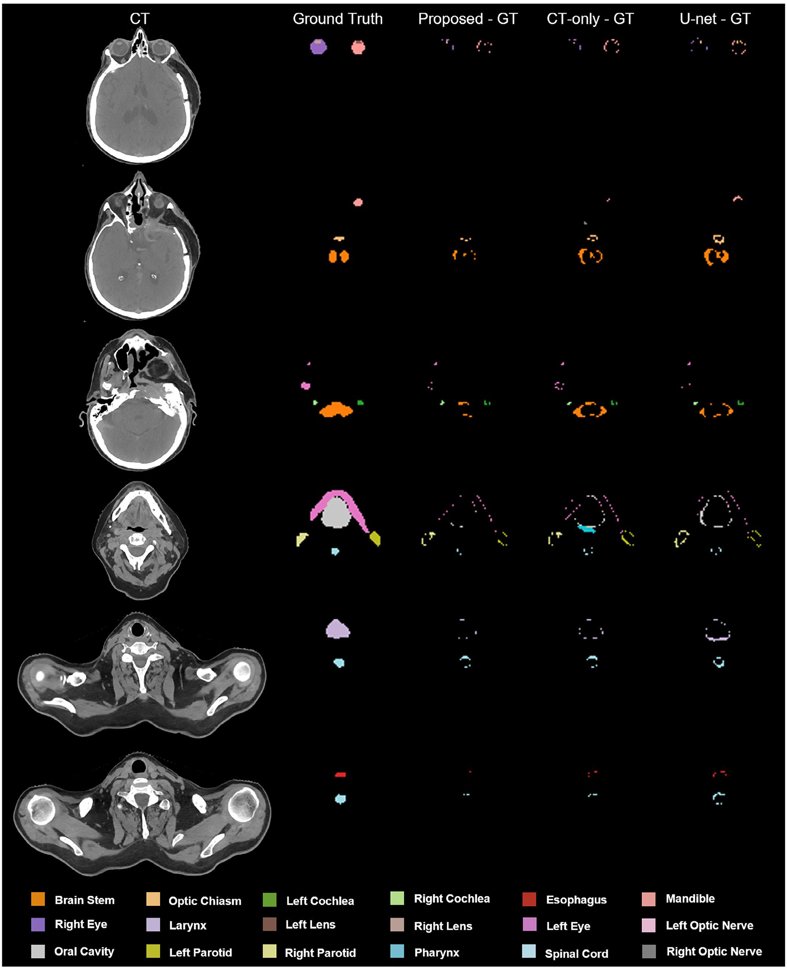
An illustrative example of the benefit of our proposed method (MS-RCNN with sMRI) compared with MS-RCNN without sMRI, and U-net with sMRI. Proposed – GT, the discrepancy between proposed method prediction and ground truth, computed tomography (CT)-only – GT, the discrepancy between CT-only method prediction and ground truth, U-net – GT, the discrepancy between U-net method prediction and ground truth

FIGURE 3.

An illustrative example of the complementary contrasts obtained from synthetic magnetic resonance imaging (sMRI). (a1)-(c1) are three transversal slices of computed tomography (CT), MRI, sMRI, and ground truth contour images. (a2) and (a3) are the profiles of CT, MRI, and sMRI along the dashed lines in (a1), (b2)-(b4) show the profiles of CT, MRI, and sMRI along the dashed lines in (b1), and (c2) is the profiles of CT, MRI, and sMRI along the dashed lines in (c1)

TABLE 1.

Dice similarity coefficient (DSC) comparison of the proposed, computed tomography (CT)-only, and U-net methods on in-house dataset

Organ	I. Proposed	II. CT-only	III. U-net	p value (I vs II)	p value (I vs III)
Brain Stem	0.90±0.06	0.86±0.06	0.87±0.04	<0.01	<0.01
Left Cochlea	0.67±0.21	0.66±0.19	0.60±0.26	0.14	0.07
Right Cochlea	0.67±0.21	0.66±0.18	0.60±0.24	0.13	0.07
Esophagus	0.85±0.12	0.81±0.12	0.84±0.07	<0.01	0.19
Left Eye	0.78±0.23	0.78±0.25	0.74±0.28	0.84	0.40
Right Eye	0.76±0.26	0.76±0.27	0.72±0.30	0.99	0.37
Larynx	0.88±0.10	0.82±0.17	0.84±0.17	<0.01	0.03
Left Lnns	0.79±0.10	0.77±0.14	0.71±0.19	0.38	<0.01
Right nens	0.77±0.10	0.75±0.12	0.62±0.25	0.29	<0.01
Mandible	0.89±0.10	0.85±0.10	0.88±0.08	<0.01	0.22
Optic Chiasm	0.58±0.25	0.50±0.24	0.54±0.20	<0.01	0.12
Left Optic Nerve	0.66±0.17	0.64±0.19	0.63±0.22	0.42	0.24
Right Optic Nerve	0.66±0.20	0.63±0.20	0.60±0.23	0.40	0.06
Oral Cavity	0.89±0.10	0.83±0.12	0.85±0.12	<0.01	0.02
Left Parotid	0.83±0.09	0.83±0.09	0.75±0.27	0.49	0.02
Right Parotid	0.82±0.13	0.82±0.14	0.75±0.25	0.47	0.04
Pharynx	0.68±0.27	0.62±0.28	0.65±0.27	<0.01	<0.01
Spinal Cord	0.86±0.07	0.82±0.08	0.84±0.05	<0.01	<0.01

Note: Bold indicates the best performance achieved among the comparing methods.

FIGURE 4.

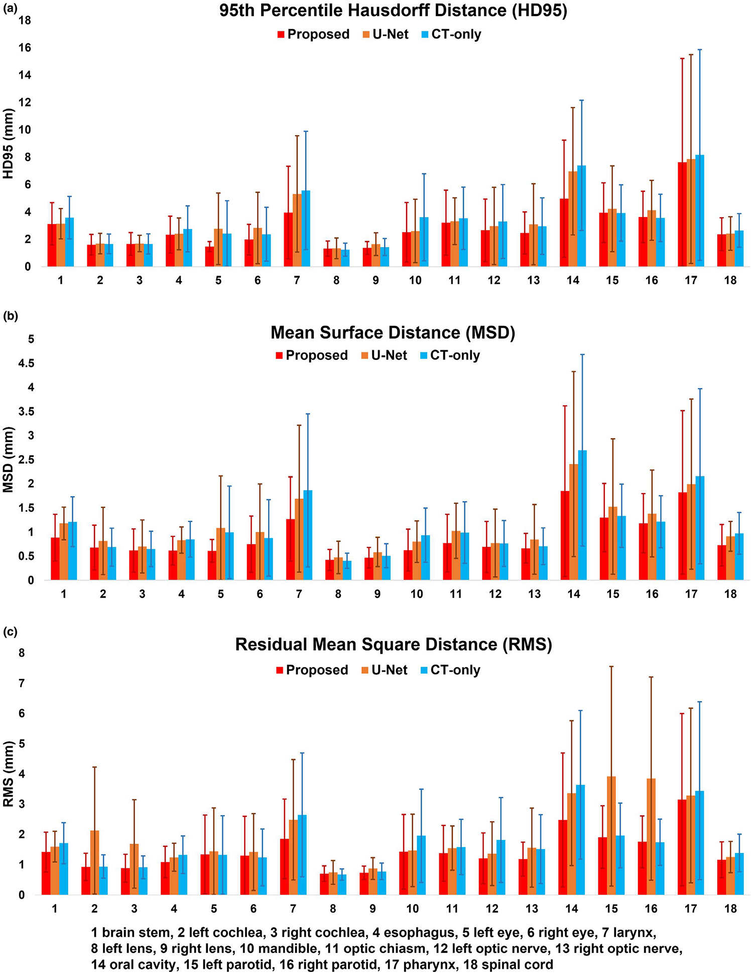
Comparisons of the proposed, computed tomography-only, and U-net methods in metrics including 95th percentile Hausdorff distance, mean surface distance, and residual mean square distance for in-house dataset

TABLE 2.

Results of paired student t-test (p-value) among the computed tomography (CT)-only, U-net, and the proposed methods on in-house dataset

Organ	Method	HD95	MS.	RMS
Brain Stem	Proposed vs CT-only	<0.01	<0.01	<0.01
	Proposed vs U-net	0.93	<0.01	<0.01
Left Cochlea	Proposed vs CT-only	0.05	0.47	0.46
	Proposed vs U-net	0.36	0.09	0.07
Right Cochlea	Proposed vs CT-only	0.89	0.07	0.08
	Proposed vs U-net	0.79	0.30	0.06
Esophagus	Proposed vs CT-only	<0.01	<0.01	<0.01
	Proposed vs U-net	0.66	0.06	0.06
Left Eye	Proposed vs CT-only	0.06	0.11	0.97
	Proposed vs U-net	0.06	0.07	0.81
Right Eye	Proposed vs CT-only	0.27	0.35	0.95
	Proposed vs U-net	0.08	0.17	0.62
Larynx	Proposed vs CT-only	<0.01	<0.01	<0.01
	Proposed vs U-net	<0.01	0.01	<0.01
Left Lens	Proposed vs CT-only	0.17	0.31	0.20
	Proposed vs U-net	0.04	0.01	0.04
Right Lens	Proposed vs CT-only	0.52	0.30	0.36
	Proposed vs U-.et	0.04	<0.01	0.01
Mandible	Proposed vs CT-only	<0.01	<0.01	<0.01
	Proposed vs U-net	0.72	0.06	0.59
Optic Chiasm	Proposed vs CT-only	<0.01	<0.01	<0.01
	Proposed vs U-n.t	0.64	0.05	0.05
Left Optic Nerve	Proposed vs CT-only	0.13	0.40	0.06
	Proposed vs U-net	0.09	0.07	0.06
Right Optic Nerve	Proposed vs CT-only	0.31	0.63	0.19
	Proposed vs U-net	0.37	0.19	0.15
Oral Cavity	Proposed vs CT-only	<0.01	<0.01	<0.01
	Proposed vs U-net	<0.01	0.02	<0.01
Left Parotid	Proposed vs CT-only	0.74	0.05	0.26
	Proposed vs U-net	0.03	0.03	0.04
Right Parotid	Proposed vs CT-only	0.12	0.09	0.71
	Proposed vs U-net	0.02	0.01	0.04
Pharynx	Proposed vs CT-only	<0.01	<0.01	<0.01
	Proposed vs U-net	<0.01	<0.01	<0.01
Spinal Cord	Proposed vs CT-only	<0.01	<0.01	<0.01
	Proposed vs U-ne1	<0.01	<0.01	<0.01

Table 3 summarized the DSC comparison between our proposed and the state-of-the-art methods. Except left/right parotid, our proposed method overperformed all the four state-of-the-art methods in organs including brain stem, optic chiasm, mandible, left/right optic nerve, and left/right submandibular.

TABLE 3.

Dice similarity coefficient (DSC) comparison to the published state-of-the-art methods on the 2015 PDDCA dataset

Organ	Proposed	Method of43	Method of14	Method of10	Method of44
Brain Stem	0.93 ± 0.02	0.88 ± 0.02	0.87 ± 0.03	0.87 ±0.03	0.87 ± 0. 02
Optic Chiasm	0.73 ± 0.15	0.45 ± 0.17	0.58 ± 0.1	0.62 ± 0.1	0.53 ± 0.15
Mandible	0.97 ± 0.01	0.93 ± 0.02	0.87 ± 0.03	0.95 ± 0.01	0.93 ± 0.02
Left Optic Nerve	0.80 ± 0.07	0.74 ± 0.15	0.65 ± 0.05	0.75 ± 0.07	0.72 ± 0.06
Right Optic Nerve	0.80 ± 0.08	0.74 ± 0.09	0.69 ± 0.5	0.72 ± 0.06	0.71 ± 0.1
Left Parotid	0.89 ± 0.05	0.86 ± 0.02	0.84 ± 0.02	0.89 ± 0.02	0.88 ± 0.02
Right Parotid	0.88 ± 0.06	0.85 ± 0.07	0.83 ± 0.02	0.88 ± 0.05	0.87 ± 0.04
Left Submandibular	0.88 ± 0.05	0.76 ± 0.15	0.76 ± 0.06	0.82 ± 0.05	0.81 ± 0.04
Right Submandibular	0.85 ± 0.11	0.73 ± 0.01	0.81 ± 0.06	0.82 ± 0.05	0.81 ± 0.04

Note: Bold indicates the best performance achieved among the comparing methods.

4 |. DISCUSSION

Delineation of organs-at-risk is a foundational component for radiotherapy treatment planning. Especially for those highly modulated treatment modalities such as intensity modulated radiotherapy (IMRT), stereotactic body radiotherapy (SBRT), and pencil beam protons, accuracy is essential. In this study, a new deep learning-based automated OAR delineation in the head and neck area has been presented. In terms of DSC score, our proposed method improved the delineation accuracy over the competing methods by 6% using our in-house dataset, and over the published state-of-the-art methods by 6% using public benchmark dataset, respectively. For the cross-validation using in-house dataset, the proposed method achieved even higher improvements in terms of HD95 (16%), MSD (25%), and RMS (36%).

The promising results can be attributed to two features of the proposed method. In contrast to most existing deep learning models for HN segmentation, which primarily rely on extracting features from only CT data,^14–17 a pre-trained cycleGAN was used in the proposed method to generate a synthetic MRI from CT. Next, both the CT and synthetic MRI were simultaneously fed into the model for segmentation, thereby leveraging the soft tissue features of the synthetic MRI and the bony contrast of the CT. Further the synthetic MRI is not subject to co-registration errors from independent MRI and CT datasets which can degrade segmentation accuracy. The second key feature is the two-stage-in-one design of the network architecture, which outperformed most existing deep learning algorithms based on U-net or its variants. In our model, the initial candidate ROIs were determined by 3D dual pyramid networks as the backbone and a regional proposal network. Then the final contours were obtained by a refining stage constructed by a regional convolutional neural network head, a mask head, and a mask score head working on those coarse initial ROIs. Even though this complex two-stage-in-one network architecture could increase the computational time for the initial model training, once the model is well trained, the automatic contour delineation is as fast as existing algorithms.

Despite these encouraging results, there are study limitations worth noting. As seen in Table 3, for a majority of organs, our proposed method achieved better results. But for left/right parotid, our proposed method achieved comparable mean DSC but a larger standard deviation compared to the reported method.¹⁴ In MS-RCNN, a set of anchors (used as potential ROIs) have to be pre-defined. RPN was used to predict the relationship between these anchors and organ ROIs. RCNN was then used to adjust the position of each detected ROI. By using anchors, the features used for ROI detection and segmentation within ROI is cropped within the anchors, thus the global spatial correlation between organs could be missing as compared to those fully convolutional networks.¹⁴ Besides, in the training process, manual contours were used as the ground truth. Uncertainty is unavoidable in the manual contouring process. Inter-observer variations still exist among experts.¹⁴ Ideally, standardized benchmark datasets would be used to evaluate the performance of all deep learning-based segmentation algorithms. One possible way to build this type of benchmark dataset is to derive contours for a common case from an ensemble of contours from multiple experts at multiple institutions, each following the same guidelines. Another method is to build a large dataset, by which, the model is expected to minimize the uncertainty in the ground truth. These limitations noted, we assessed the performance of our proposed method through comparisons between the predictions and an imperfect ground truth. The general framework of the model can easily accept consensus datasets or larger datasets.

5 |. CONCLUSIONS

We developed a synthetic MRI-aided deep learning framework for automated delineation of OARs in HN radiotherapy treatment planning. The proposed network provides accurate and consistent segmentation up to 18 organs, and has the potential to facilitate routine radiotherapy treatment planning.

DATA AVAILABILITY STATEMENT

The data that support the findings of this study are available on request from the corresponding author. The data are not publicly available due to privacy or ethical restrictions.

REFERENCES

- 1.Harari PM, Song S, Tome WA. Emphasizing conformal avoidance versus target definition for IMRT planning in head-and-neck cancer [published online ahead of print 2010/04/10]. Int J Radiat Oncol Biol Phys. 2010;77(3):950–958. [DOI] [PMC free article] [PubMed] [Google Scholar]
- 2.Brouwer CL, Steenbakkers RJHM, van den Heuvel E, et al. 3D Variation in delineation of head and neck organs at risk. Radiat Oncol. 2012;7(1):32. [DOI] [PMC free article] [PubMed] [Google Scholar]
- 3.Brouwer CL, Steenbakkers RJHM, Bourhis J, et al. CT-based delineation of organs at risk in the head and neck region: DAHANCA, EORTC, GORTEC, HKNPCSG, NCIC CTG, NCRI, NRG Oncology and TROG consensus guidelines. Radiother Oncol. 2015;117(1):83–90. [DOI] [PubMed] [Google Scholar]
- 4.Walker GV, Awan M, Tao R, et al. Prospective randomized double-blind study of atlas-based organ-at-risk autosegmentation-assisted radiation planning in head and neck cancer [published online ahead of print 2014/09/14]. Radiother Oncol 2014;112(3):321–325. [DOI] [PMC free article] [PubMed] [Google Scholar]
- 5.Kosmin M, Ledsam J, Romera-Paredes B, et al. Rapid advances in auto-segmentation of organs at risk and target volumes in head and neck cancer. Radiother Oncol. 2019;135:130–140. [DOI] [PubMed] [Google Scholar]
- 6.Daisne J-F, Blumhofer A Atlas-based automatic segmentation of head and neck organs at risk and nodal target volumes: a clinical validation. Radiat Oncol. 2013;8(1):154. [DOI] [PMC free article] [PubMed] [Google Scholar]
- 7.Hoogeman MS, Han X, Teguh D, et al. Atlas-based auto-segmentation of CT images in head and neck cancer: what is the best approach? Int J Radiat Oncol Biol Phys. 2008;72(1):S591. [Google Scholar]
- 8.Levendag PC, Hoogeman M, Teguh D, et al. Atlas based auto-segmentation of ct images: clinical evaluation of using auto-contouring in high-dose, high-precision radiotherapy of cancer in the head and neck. Int J Radiat Oncol Biol Phys. 2008;72(1):S401. [Google Scholar]
- 9.Dai X, Lei Y, Wang T, et al. Self-supervised learning for accelerated 3D high-resolution ultrasound imaging [published online ahead of print 2021/05/17]. Med Phys. 2021;48(7):3916–3926. 10.1002/mp.14946. [DOI] [PMC free article] [PubMed] [Google Scholar]
- 10.Dai X, Lei Y, Liu Y, et al. Intensity non-uniformity correction in MR imaging using residual cycle generative adversarial network [published online ahead of print 2020/11/28]. Phys Med Biol. 2020;65(21):215025. [DOI] [PMC free article] [PubMed] [Google Scholar]
- 11.Dai X, Lei Y, Fu Y, et al. Multimodal MRI synthesis using unified generative adversarial networks [published online ahead of print 2020/10/15]. Med Phys. 2020;47(12):6343–6354. [DOI] [PMC free article] [PubMed] [Google Scholar]
- 12.Xing L, Giger ML, Min JK. Artificial intelligence in medicine: technical basis and clinical applications. Academic Press; 2020. [Google Scholar]
- 13.Lin LI, Dou QI, Jin Y-M, et al. Deep learning for automated contouring of primary tumor volumes by MRI for nasopharyngeal carcinoma [published online ahead of print 2019/03/27]. Radiology. 2019;291(3):677–686. [DOI] [PubMed] [Google Scholar]
- 14.Tang H, Chen X, Liu Y, et al. Clinically applicable deep learning framework for organs at risk delineation in CT images. Nat Mach Int. 2019;1(10):480–491. [Google Scholar]
- 15.van Rooij W, Dahele M, Brandao HR, Delaney AR, Slotman BJ, Verbakel WF. Deep learning-based delineation of head and neck organs at risk: geometric and dosimetric evaluation. Int J Radiat Oncol Biol Phys. 2019;104(3):677–684. [DOI] [PubMed] [Google Scholar]
- 16.Guo D, Jin D, Zhu Z, et al. Organ at Risk Segmentation for Head and Neck Cancer using Stratified Learning and Neural Architecture Search. Paper presented at: Proceedings of the IEEE/CVF Conference on Computer Vision and Pattern Recognition; 2020. [Google Scholar]
- 17.van Dijk LV, Van den Bosch L, Aljabar P, et al. Improving automatic delineation for head and neck organs at risk by Deep Learning Contouring. Radiother Oncol. 2020;142:115–123. [DOI] [PubMed] [Google Scholar]
- 18.Tong N, Gou S, Yang S, Ruan D, Sheng K. Fully automatic multi-organ segmentation for head and neck cancer radiotherapy using shape representation model constrained fully convolutional neural networks. Med Phys. 2018;45(10):4558–4567. [DOI] [PMC free article] [PubMed] [Google Scholar]
- 19.Sahiner B, Pezeshk A, Hadjiiski LM, et al. Deep learning in medical imaging and radiation therapy [published online ahead of print 2018/10/28]. Med Phys. 2019;46(1):e1–e36. [DOI] [PMC free article] [PubMed] [Google Scholar]
- 20.van der Veen J, Willems S, Deschuymer S, et al. Benefits of deep learning for delineation of organs at risk in head and neck cancer. Radiother Oncol. 2019;138:68–74. [DOI] [PubMed] [Google Scholar]
- 21.Seo H, Badiei Khuzani M, Vasudevan V, et al. Machine learning techniques for biomedical image segmentation: An overview of technical aspects and introduction to state-of-art applications. Med Phys. 2020;47(5):e148–e167. [DOI] [PMC free article] [PubMed] [Google Scholar]
- 22.Dai X, Lei Y, Wang T, et al. Head-and-neck organs-at-risk auto-delineation using dual pyramid networks for CBCT-guided adaptive radiotherapy [published online ahead of print 2021/01/08]. Phys Med Biol. 2021;66(4):045021. [DOI] [PMC free article] [PubMed] [Google Scholar]
- 23.Ibragimov B, Xing L. Segmentation of organs-at-risks in head and neck CT images using convolutional neural networks. Med Phys. 2017;44(2):547–557. [DOI] [PMC free article] [PubMed] [Google Scholar]
- 24.Zhou X, Takayama R, Wang S, Hara T, Fujita H. Deep learning of the sectional appearances of 3D CT images for anatomical structure segmentation based on an FCN voting method [published online ahead of print 2017/07/22]. Med Phys. 2017;44(10):5221–5233. [DOI] [PubMed] [Google Scholar]
- 25.Weston AD, Korfiatis P, Kline TL, et al. Automated abdominal segmentation of CT scans for body composition analysis using deep learning. Radiology. 2019;290(3):669–679. [DOI] [PubMed] [Google Scholar]
- 26.Gibson E, Giganti F, Hu Y, et al. Automatic multi-organ segmentation on abdominal CT with Dense V-Networks [published online ahead of print 2018/07/12]. IEEE Trans Med Imaging. 2018;37(8):1822–1834. [DOI] [PMC free article] [PubMed] [Google Scholar]
- 27.Seo H, Huang C, Bassenne M, Xiao R, Xing L. Modified U-Net (mU-Net) with incorporation of object-dependent high level features for improved liver and liver-tumor segmentation in CT images. IEEE Trans Med Imaging. 2019;39(5):1316–1325. [DOI] [PMC free article] [PubMed] [Google Scholar]
- 28.Wang S, He K, Nie D, Zhou S, Gao Y, Shen D. CT male pelvic organ segmentation using fully convolutional networks with boundary sensitive representation. Med Image Anal. 2019;54:168–178. [DOI] [PMC free article] [PubMed] [Google Scholar]
- 29.Kazemifar S, Balagopal A, Nguyen D, et al. Segmentation of the prostate and organs at risk in male pelvic CT images using deep learning. Biomed Phys Eng Exp. 2018;4(5):055003. [Google Scholar]
- 30.Dong X, Lei Y, Tian S, et al. Synthetic MRI-aided multi-organ segmentation on male pelvic CT using cycle consistent deep attention network. Radiother Oncol. 2019;141:192–199. [DOI] [PMC free article] [PubMed] [Google Scholar]
- 31.Khoo VS, Joon DL. New developments in MRI for target volume delineation in radiotherapy [published online ahead of print 2006/09/19]. Br J Radiol. 2006;79(special_issue_1):S2–S15. [DOI] [PubMed] [Google Scholar]
- 32.Das IJ, McGee KP, Tyagi N, Wang H. Role and future of MRI in radiation oncology [published online ahead of print 2018/11/02]. Br J Radiol. 2019;92(1094):20180505. [DOI] [PMC free article] [PubMed] [Google Scholar]
- 33.Lei Y, Dong X, Tian Z, et al. CT prostate segmentation based on synthetic MRI-aided deep attention fully convolution network [published online ahead of print 2019/11/21]. Med Phys. 2020;47(2):530–540. [DOI] [PMC free article] [PubMed] [Google Scholar]
- 34.Zhu J-Y, Park T, Isola P, Efros AA. Unpaired image-to-image translation using cycle-consistent adversarial networks. Paper presented at: Proceedings of the IEEE international conference on computer vision; 2017. [Google Scholar]
- 35.Lei Y, He X, Yao J, et al. Breast tumor segmentation in 3D automatic breast ultrasound using Mask scoring R-CNN [published online ahead of print 2020/11/01]. Med Phys. 2021;48(1):204–214. [DOI] [PubMed] [Google Scholar]
- 36.Lei Y, Harms J, Wang T, et al. MRI-only based synthetic CT generation using dense cycle consistent generative adversarial networks. Med Phys. 2019;46(8):3565–3581. [DOI] [PMC free article] [PubMed] [Google Scholar]
- 37.Ronneberger O, Fischer P, Brox T. U-net: Convolutional networks for biomedical image segmentation. Paper presented at: International Conference on Medical image computing and computer-assisted intervention; 2015. [Google Scholar]
- 38.Zhang Z, Sabuncu MR. Generalized cross entropy loss for training deep neural networks with noisy labels. arXiv preprint arXiv:07836. 2018. [Google Scholar]
- 39.Girshick R, Donahue J, Darrell T, Malik J. Rich feature hierarchies for accurate object detection and semantic segmentation. Paper presented at: Proceedings of the IEEE conference on computer vision and pattern recognition; 2014. [Google Scholar]
- 40.Ren S, He K, Girshick R, Sun J. Faster r-cnn: Towards real-time object detection with region proposal networks. Paper presented at: Advances in neural information processing sytems; 2015. [DOI] [PubMed] [Google Scholar]
- 41.Cui Y, Jia M, Lin T-Y, Song Y, Belongie S. Class-balanced loss based on effective number of samples. Paper presented at: Proceedings of the IEEE/CVF Conference on Computer Vision and Pattern Recognition; 2019. [Google Scholar]
- 42.Huang Z, Huang L, Gong Y, Huang C, Wang X. Mask scoring r-cnn. Paper presented at: Proceedings of the IEEE conference on computer vision and pattern recognition; 2019. [Google Scholar]
- 43.Dai X, Lei Y, Zhang Y, et al. Automatic multi-catheter detection using deeply supervised convolutional neural network in MRI-guided HDR prostate brachytherapy. Med Phys 2020;47(9):4115–4124. [DOI] [PMC free article] [PubMed] [Google Scholar]
- 44.He K, Gkioxari G, Dollár P, Girshick R. Mask r-cnn. Paper presented at: Proceedings of the IEEE international conference on computer vision; 2017. [Google Scholar]
- 45.Jaeger PF, Kohl SA, Bickelhaupt S, et al. Retina U-Net: Embarrassingly simple exploitation of segmentation supervision for medical object detection. arXiv preprint arXiv:181108661. 2018. [Google Scholar]
- 46.Raudaschl PF, Zaffino P, Sharp GC, et al. Evaluation of segmentation methods on head and neck CT: auto-segmentation challenge 2015 [published online ahead of print 2017/03/09]. Med Phys. 2017;44(5):2020–2036. [DOI] [PubMed] [Google Scholar]
Associated Data
This section collects any data citations, data availability statements, or supplementary materials included in this article.
Supplementary Materials