Enhancing Cure Rate Analysis Through Integration of Machine Learning Models: A Comparative Study

Abstract

Cure rate models have been thoroughly investigated across various domains, encompassing medicine, reliability, and finance. The merging of machine learning (ML) with cure models is emerging as a promising strategy to improve predictive accuracy and gain profound insights into the underlying mechanisms influencing the probability of cure. The current body of literature has explored the benefits of incorporating a single ML algorithm with cure models. However, there is a notable absence of a comprehensive study that compares the performances of various ML algorithms in this context. This paper seeks to address and bridge this gap. Specifically, we focus on the well-known mixture cure model and examine the incorporation of five distinct ML algorithms: extreme gradient boosting, neural networks, support vector machines, random forests, and decision trees. To bolster the robustness of our comparison, we also include cure models with logistic and spline-based regression. For parameter estimation, we formulate an expectation maximization algorithm. A comprehensive simulation study is conducted across diverse scenarios to compare various models based on the accuracy and precision of estimates for different quantities of interest, along with the predictive accuracy of cure. The results derived from both the simulation study, as well as the analysis of real cutaneous melanoma data, indicate that the incorporation of ML models into cure model provides a beneficial contribution to the ongoing endeavors aimed at improving the accuracy of cure rate estimation.

1. Introduction

Cure rate analysis, a statistical methodology, is employed to identify a sub-group of individuals within a population who are immuned to a specific event of interest, such as disease recurrence or mortality with respect to a certain condition, thus exhibiting a “cure” response (Maller & Zhou, 1996; Balakrishnan & Pal, 2013, 2015, 2016; Peng & Yu, 2021, Pal & Roy, 2021, 2022, 2023). The study of cure models, which are models to analyze time-to-event data consisting of a cured subgroup, has become an invaluable area of research in recent times due to the numerous applications of cure models in medicine and epidemiology, engineering, criminology, sociology, and finance, among others. For example, in healthcare and medicine, precise estimates of cure rates can prevent patients from going through unnecessary treatments which may have toxic effects, thereby leading to more personalized and effective healthcare strategies (Levine et al., 2005, Liu et al., 2012). Understanding factors that significantly contribute to the estimation of cure rates can provide valuable insights into disease dynamics and inform public health interventions (Peng & Dear, 2000; Pal & Balakrishnan, 2017a b; Pal, 2021; Treszoks & Pal, 2023, 2024). Similarly, in finance, those customers who would never default on a loan can be considered as cured. Thus, cure models can help mitigate risks associated with loan defaults and financial distress (Jiang et al., 2019). Again, in criminology, the effectiveness of rehabilitation in deterring offenders from recommitting crimes hinges significantly on the recidivism rate. In this regard, those subjects who would never commit a crime again can be considered cured and hence cure models play a big role in predicting these subjects and identifying the associated factors (Treszoks & Pal, 2022; de la Cruz et al., 2022). Thus, we see that even though the term “cure” sounds biomedical, cure models have diverse applications across various disciplines.

The mixture cure model (MCM) stands out as the most frequently employed cure model (Boag. 1949; Berkson & Gage, 1952; Farewell, 1986). This type of model is particularly relevant in situations where a proportion of individuals in the population under study will never experience the event of interest, leading to a “cured” state. MCM helps to account for heterogeneity in the population and provides insights into both the probability of being susceptible to an event of interest and the probability of being cured. Let $U$ denote the cured status, defined as $U=0$ if a subject is cured and $U=1$ if a subject is susceptible or uncured. Further, let $T^{*}$ denote the lifetime of an uncured subject. Then, we can define the lifetime, $T$, for any subject in the mixture population as

$$T=U{T}^{*}+(1-U)\infty .$$ (1)

In addition, let the survival function of $T^{*}$ be denoted by $S_u(\cdot )$, i.e., $S_u\left(t\right)=P\left(T^{*}>t\right)$. Thus, we can express the survival function of the mixture population, denoted by $S_p(\cdot )$, as

$$S_p\left(t\right)=\left(1-\pi \right)+\pi S_u\left(t\right),$$ (2)

where $1-\pi =P(U=0)$ denotes the cured probability. To incorporate covariate structure into the MCM in (1), let $\mathit{x}$ denote a covariate vector associated with the survival distribution of the susceptible subject (also known as the latency), i.e., $S_u\left(t\right)=S_u(t;\mathit{x})$. Also, let $\mathit{z}$ denote another covariate vector associated with the cure/uncure probability (also known as the incidence), i.e., $\pi =\pi \left(\mathit{z}\right)$. Observe that $\mathit{x}$ and $\mathit{z}$ may have full, partial, or no overlap.

The conventional method of modeling $\pi \left(\mathit{z}\right)$ or $1-\pi \left(\mathit{z}\right)$ involves assuming a logistic link function, i.e.,

$$\pi \left(\mathit{z}\right)=\frac{\text{exp}\left({\mathit{z}}^{\prime }\mathit{\gamma }\right)}{1+\text{exp}\left({\mathit{z}}^{\prime }\mathit{\gamma }\right)},$$ (3)

where $\mathit{\gamma }$ denotes the vector of regression coefficients including an intercept term (Peng & Dear, 2000). Other alternate modeling strategies include the use of probit link function $\left({\Phi }^{-1}\left(\pi \right(\mathit{z}\left)\right)={\mathit{z}}^{\prime }\mathit{\gamma }\right)$ or the complementary log-log link function $\left(\text{log}[-\text{log}(1-\pi \left(\mathit{z}\right)\left)\right]={\mathit{z}}^{\prime }\mathit{\gamma }\right)$, where $\Phi$ denotes the cumulative distribution function of the standard normal distribution (Peng, 2003; Cai et al., 2012; Tong et al., 2012). The performances of the aforementioned link functions are similar and they facilitate a straightforward interpretation of how $\mathit{z}$ affect $\pi \left(\mathit{z}\right)$. However, a major drawback of these link functions is that they cannot capture complex effects of $\mathit{z}$ on $\pi \left(\mathit{z}\right)$. Other non-parametric approaches to model the effect of $\mathit{z}$ on $\pi \left(\mathit{z}\right)$ are feasible only for a single covariate (Xu & Peng, 2014, López-Cheda et al., 2017). Similarly, spline-based approaches have shown some promise, however, they may not perform well in the presence of a large number of covariates with complicated interaction terms (Chen & Du, 2018). Hence, there is considerable space for enhancing the modeling strategies for the incidence component of the MCM.

The integration of machine learning (ML) algorithms with cure models has gained significant attention in recent years across various research domains. Such an integration offers the potential to enhance the accuracy and predictive power of identifying the “cured” sub-group within the population. ML models are renowned for their ability to uncover intricate patterns and relationships within datasets, making them promising candidates for improving the predictive accuracy of cure. The pioneering work that effectively integrated ML algorithm with cure model is by Li et al. (2020), where the authors proposed the support vector machine (SVM) classifier to model the incidence part of MCM. It was shown that the SVM-based MCM outperforms the existing logistic regression-based MCM. Xie & Yu (2021a) used neural networks (NN) to capture complex unstructured covariate effect on the incidence part of MCM. The authors estimated the model parameters through the development of an expectation maximization (EM) algorithm and showed consistency of the estimators; see also Xie & Yu (2021b) and Pal & Aselisewine (2023). Later, Aselisewine & Pal (2023) used the decision trees (DT) to model the incidence part of MCM and showed their model to perform better when compared to both logistic regression-based and spline-based MCM models. Pal, Peng, & Aselisewine (2023) and Pal, Peng, Aselisewine, & Barui (2023) extended the previous work of Li et al. (2020) by considering the form of the observed data to be interval censored. An EM algorithm was developed in the presence of interval censored data and the superiority of the proposed models was demonstrated.

To the best of our knowledge there does not exist any comprehensive study comparing the performances of different ML algorithms in the context of modeling the incidence part of MCM. To fill this gap, in this work, we propose to model the incidence part of MCM using some well-known ML-based classifiers such as the Extreme Gradient Boosting (XGB), Random Forests (RF), NN, SVM, and DT, which can capture complex relationship between $\mathit{z}$ and $\pi \left(\mathit{z}\right)$. ML models are well known for their ability to uncover intricate patterns and relationships in data analysis, and by integrating them with cure model we stand to gain not only the improvement in the predictive capabilities of cure rate analysis but also unlock a deeper insights into the mechanisms underlying the probability of cure. Studying each of these ML-based MCM models will help us explore and discover distinct advantages and disadvantages associated with each underlying model. Note, however, that by bringing in ML-based approaches we sacrifice the easy interpretation of the effect of covariates on the incidence that, for example, a logistic regression-based model may provide. In this regard, we retain the proportional hazards (PH) structure on the latency part, which allows for a simple interpretation of covariate effect on the survival distribution of the uncured subjects. We develop an EM algorithm to estimate model parameters for each ML-based MCM under consideration McLachlan & Krishnan (2007). The performances of the ML-based MCM models, together with the traditional logistic regression-based MCM and spline-based MCM, are evaluated and compared using both simulated data and real data.

The rest of this article is organized as follows. In Section 2, we discuss the form of the data and our modeling strategies for the incidence and latency parts of the MCM. In Section 3, we outline the construction of the EM algorithm used for estimating model parameters. In Section 4, we conduct a thorough simulation study and compare different models under varying scenarios and parameter settings. In Section 5, we apply the proposed models and estimation method to analyze survival data obtained from a study on cutaneous melanoma. Finally, in Section 6, we conclude with final remarks and delve into potential avenues for future research.

2. Machine learning-based mixture cure models

We examine a situation where the censoring mechanism for the observed right-censored data is non-informative. If we let $Y$ denote the true lifetime and $C$ denote the right censoring time, then, the observed lifetime, denoted by $T$, can be written as $T=\text{min}\{Y,C\}$. Furthermore, let the censoring indicator, denoted by $\delta$, take the value 1 if the true lifetime is observed (i.e., $T=Y$) and the value 0 if the true lifetime is right censored (i.e., $T=C$). The observed data are of the form $\left\{\left(t_i,{\delta }_i,{\mathit{x}}_i,{\mathit{z}}_i\right)\right.,\text{for}i=\mathrm{1,2},\cdots ,n\}$, where $n$ denotes the number of subjects in the study. Next, to incorporate the effect of covariates on the latency, we assume the lifetime distribution of the uncured subjects to follow a semi-parametric proportional hazards structure. Thus, the hazard function of the uncured subjects can be expressed as

$$h_u\left(t;\mathit{x}\right)=h_{u0}\left(t\right)\text{exp}\left({\mathit{x}}^{\prime }\mathit{\beta }\right),$$ (4)

where $\mathit{\beta }$ is a vector of regression coefficients without an intercept term and $h_{u0}(\cdot )$ is an unspecified baseline hazard function that depends only on $t$. The MCM defined in (2) can then be rewritten as

$$S_p\left(t;\mathit{x},\mathit{z}\right)=1-\pi \left(\mathit{z}\right)+\pi \left(\mathit{z}\right){\left\{S_{u0}\left(t\right)\right\}}^{\text{exp}\left({\mathit{x}}^{\prime }\mathit{\beta }\right)},$$ (5)

where $S_{u0}\left(t\right)=\text{exp}\left\{-{\int }_0^t{h}_{u0}\left(u\right)du\right\}$ is the baseline survival function. Considering the cured status $U$ as the missing data (note that $U$ is unknown if $\delta =0$), we define the complete data as $\left\{\left(t_i,{\delta }_i,U_i,{\mathit{x}}_i,{\mathit{z}}_i\right),i=\mathrm{1,2},\cdots ,n\right\}$ which includes both observed and unobserved $U_i$’s. Using the complete data, we can express the complete data likelihood function as

$$L_c=\prod _{i=1}^n{\left[{\left\{\pi \left({\mathit{z}}_i\right)f_u\left(t_i;{\mathit{x}}_i\right)\right\}}^{U_i}\right]}^{{\delta }_i}{\left[{\left\{1-\pi \left({\mathit{z}}_i\right)\right\}}^{1-U_i}{\left\{\pi \left({\mathit{z}}_i\right)S_u\left(t_i;{\mathit{x}}_i\right)\right\}}^{U_i}\right]}^{1-{\delta }_i},$$ (6)

where $S_u\left(t_i;{\mathit{x}}_i\right)={\left\{S_{u0}\left(t_i\right)\right\}}^{\text{exp}\left({\mathit{x}}_i^{\prime }\mathit{\beta }\right)}$ and $f_u\left(t_i;{\mathit{x}}_i\right)$ is the density function associated with $S_u\left(t_i;{\mathit{x}}_i\right)$. Using (6), the corresponding log-likelihood function, denoted by $l_c$, can be expressed as $l_c=l_{c1}+l_{c2}$, where

$$l_{c1}=\sum _{i=1}^n\left[U_i\text{log}\pi \left({\mathit{z}}_i\right)+\left(1-U_i\right)\text{log}\left(1-\pi \left({\mathit{z}}_i\right)\right)\right]$$ (7)

and

$$l_{c2}=\sum _{i=1}^n\left[U_i\text{log}{S}_u\left(t_i;{\mathit{x}}_i\right)+{\delta }_i\text{log}{h}_u\left(t_i;{\mathit{x}}_i\right)\right].$$ (8)

It is crucial to emphasize that $l_{c1}$ exclusively encompasses parameters linked to the incidence, while $l_{c2}$ exclusively encompasses parameters associated with the latency. Also, observe that $U_i$’s are linear in both (7) and (8).

As our objective is to enhance the predictive accuracy of cure through capturing complex patterns in the data, we employ one of the ML algorithms under consideration (i.e., XGB, NN, SVM, DT, or RF) to model $\pi \left({\mathit{z}}_i\right)$ in (7). For this purpose, one may refer to the recent works of Li et al. (2020), Xie & Yu (2021a) and Aselisewine & Pal (2023). Note, however, that a big challenge to employ a suitable ML algorithm is that the class labels (i.e., cured and uncured) are not completely available due to the missing cured statuses for all right censored observations. To address this challenge, we employ an imputation-based approach, following a methodology similar to that of Li et al. (2020). The steps involved in this imputation-based approach are described in Section 3.

It is worth mentioning that for the SVM, DT, and RF classifiers, we need to convert their predictions into well-defined calibrated posterior probabilities of cured or uncured. This can be achieved through the use of Platt scaling technique (Platt et al., 1999). On the other hand, the NN and XGB classifiers inherently produce well-defined cured/uncured probabilities. The NN classifier is controlled by an activation function parameter that can be set to a sigmoid function such that the predictions are well-defined between 0 and 1. Similarly, the XGB classifier is also controlled by the learning task parameter that specifies the learning objective and model evaluation metric. When this learning objective or loss function is set to a logistic-type function it returns class probabilities which are defined between 0 and 1.

To prevent overfitting or underfitting in the incidence part of the MCM, we divide the data into a training set and a testing set. The training set is used to train each ML-based model under consideration in the incidence part and obtain the optimal values of associated hyper-parameters. We employ the grid-search cross-validation technique to determine the hyper-parameters for each model. This technique allows us to specify a range of parameter values for each hyper-parameter and perform a $k$-fold $(k=10)$ cross validation to select the optimal hyper-parameter. The hyper-parameters involved depend on the specific ML algorithm being utilized. For example, in the case of XGB-based MCM, the hyper-parameters involved are the parameter that controls the number of trees to grow or iterations in the model fitting process and the learning rate or shrinkage parameter. The hyper-parameters for the NN-based MCM are the number of hidden layers and the number of neurons in each layer. To suit our objectives, we use a two hidden layers network with $k$ and $m$ number of neurons in the first and second layers, respectively. Similarly, for the SVM-based MCM, the hyper-parameters are the $l_2$ regularization parameter and the parameter associated with the choice of a suitable kernel function (e.g., the radial basis kernel function, which we use in this work). Again, for the DT-based MCM, the hyper-parameters under consideration are the minimum number of observations that must exist in a node before a split is attempted and the complexity parameter. Finally, for the RF-based MCM, the number of trees to grow and the number of variables randomly sampled as candidates at each split are the associated hyper-parameters. After a model is trained using the training data, we use it to make predictions on the testing data. The prediction performance of each model is then assessed using certain performance metrics such as the graphical receiver operating characteristic (ROC) curve and it’s area under the curve (AUC). Since the observations in the testing set are not used in the training process, this will provide a better objective ground for evaluating the predictive performance of each model. The best model obtained through this approach is expected to perform well when applied to a new or independent cohort of data.

3. EM algorithm

Noting that the cured statuses $U_i$ remain unknown (or missing) for subjects with right-censored lifetimes, we develop an EM algorithm renowned for effectively managing this type of data missingness. Furthermore, since the missing $U_i$’s are linear in both (7) and (8), the E-step of the EM algorithm reduces to computing the conditional mean of $U_i$ given the observed data and current values of unknown model parameters. At the $k$-th iteration of the EM algorithm, the conditional mean of $U_i$ can be expressed as

$$w_i^{\left(k\right)}={\delta }_i+\left(1-{\delta }_i\right)\frac{{\pi }^{(k-1)}\left({\mathit{z}}_i\right)S_u^{(k-1)}\left(t_i;{\mathit{x}}_i\right)}{1-{\pi }^{(k-1)}\left({\mathit{z}}_i\right)+{\pi }^{(k-1)}\left({\mathit{z}}_i\right)S_u^{(k-1)}\left(t_i;{\mathit{x}}_i\right)},i=1,\cdots ,n,$$ (9)

where $S_u^{(k-1)}\left(t_i;{\mathit{x}}_i\right)={\left\{S_{u0}^{(k-1)}\left(t_i\right)\right\}}^{\text{exp}\left(x_i^{\prime }{\beta }^{(k-1)}\right)}$. It is evident that $w_i^{(k)}$ can be interpreted as the conditional probability of a subject being uncured. With the $w_i^{\left(k\right)}$’s and noting that ${\delta }_i\text{log}{w}_i^{\left(k\right)}=0$ and ${\delta }_i{w}_i^{\left(k\right)}={\delta }_i$, the E-step replaces $l_{c1}$ and $l_{c2}$ by the following functions:

$$Q_1=\sum _{i=1}^n\left[w_i^{\left(k\right)}\text{log}\pi \left({\mathit{z}}_i\right)+\left(1-w_i^{\left(k\right)}\right)\text{log}\left(1-\pi \left({\mathit{z}}_i\right)\right)\right]$$ (10)

and

$$Q_2=\sum _{i=1}^n\left[w_i^{\left(k\right)}\text{log}{S}_u\left(t_i;{\mathit{x}}_i\right)+{\delta }_i\text{log}\left\{w_i^{\left(k\right)}{h}_u\left(t_i;{\mathit{x}}_i\right)\right\}\right].$$ (11)

In the M-step of the EM algorithm, the conventional procedure involves solving two maximization problems separately; one in relation to $Q_1$ to obtain improved estimates of $\pi \left({\mathit{z}}_i\right)$ after assuming a generalized linear model for $\pi \left({\mathit{z}}_i\right)$ incorporating a parametric link function such as the logit link function, and the other in relation to $Q_2$ to obtain improved estimates of ($\mathit{\beta },S_{u0}(\cdot )$). However, in this work, we do not assume a parametric model for $\pi \left({\mathit{z}}_i\right)$. Instead, we estimate $\pi \left({\mathit{z}}_i\right)$ using a suitable ML method among the ones considered. Now, to employ a ML method, we must know the class labels (i.e., the cured and uncured statuses) for all subjects. But, as discussed earlier, the cured/uncured statuses (i.e., $U_i$’s) are unknown for all right censored observations. To overcome this challenge, we follow the suggestion of Li et al. (2020) and impute the missing $U_i$’s. At the $k$-th iteration of the EM algorithm, the imputation technique is outlined as follows. First, select the number of imputations, say $N$, and simulate $\left\{U_i^{\left(r\right)},i=1,\cdots ,n;r=1,\cdots ,N\right\}$ by sampling from a Bernoulli distribution with success probability $w_i^{\left(k\right)}$. Then, using the simulated $\left\{U_i^{\left(r\right)},i=1,\cdots ,n\right\}$ for each $r=1,\cdots ,N$, estimate $\pi \left({\mathit{z}}_i\right)$ by using the ML method being employed. Let us represent these estimates as $\widehat{{\pi }^{\left(r\right)}\left({\mathit{z}}_i\right)},r=\mathrm{1,2},\cdots ,N$. The final estimate of $\pi \left({\mathit{z}}_i\right)$ can be calculated as $\widehat{\pi \left({\mathit{z}}_i\right)}=\frac{1}{N}{\sum }_{r=1}^N\widehat{{\pi }^{\left(r\right)}\left({\mathit{z}}_i\right)}$. In practical terms, we can opt for a set of 5 imputations, i.e., $N=5$; see Li et al. (2020).

Regarding the maximization of $Q_2$, we follow the approach of Peng & Dear (2000) and approximate the estimating equation (11) by the following partial log-likelihood function:

$$\sum _{j=1}^{n_k}\text{log}\frac{\text{exp}\left(s_j^{\prime }\mathit{\beta }\right)}{{\left[\sum _{i^{\prime }\in R_j}{w}_{i^{\prime }}^{\left(k\right)}\text{exp}\left({\mathit{x}}_{i^{\prime }}^{\prime }\mathit{\beta }\right)\right]}^{d_j}}.$$ (12)

In (12), ${\tau }_1<{\tau }_2<\cdots <{\tau }_{n_k}$ are $n_k$ distinct ordered complete failure times, $d_j$ denotes number of uncensored failure times equal to ${\tau }_j,R_j$ denotes the risk set at ${\tau }_j$, and ${\mathit{s}}_j={\sum }_{\left\{\left\{i:t_i={\tau }_j\right\}\right.}{\mathit{x}}_i$, for $1\le j\le n_k$. Given the form of (12), i.e., (12) being independent of the baseline survival function, we use the “coxph()” function in R software to estimate $\mathit{\beta }$, considering $\text{log}{w}_i^{\left(k\right)}$ as an offset variable (i.e., coefficient fixed at unity). Using the estimate of $\mathit{\beta }$, the baseline survival function $S_{u0}(\cdot )$ can be estimated by the following Breslow-type estimator:

$${\widehat{S_{u0}}}^{\left(k\right)}\left(t_i\right)=\text{exp}\left(-\sum _{j:{\tau }_j<t_i}\frac{d_j}{\sum _{i^{\prime }\in R_j}{w}_{i^{\prime }}^{\left(k\right)}\text{exp}\left({\mathit{x}}_{i^{\prime }}^{\prime }{\stackrel{\mathit{ˆ}}{\mathit{\beta }}}^{\left(k\right)}\right)}\right).$$ (13)

Note that when we use (13), we must consider ${\widehat{S_{u0}}}^{\left(k\right)}\left(t_i\right)$ to be 0 if $t_i>{\tau }_{n_k}$. Using ${\widehat{S_{u0}}}^{\left(k\right)}\left(t_i\right)$, we estimate the survival function of the non-cured subjects as:

$${\widehat{S_u}}^{\left(k\right)}\left(t_i;{\mathit{x}}_i\right)={\widehat{S_{u0}}}^{\left(k\right)}{\left(t_i\right)}^{\text{exp}\left({\mathit{x}}_i^{\prime }{\stackrel{\mathit{ˆ}}{\mathit{\beta }}}^{\left(k\right)}\right)}.$$ (14)

The E- and M-steps are iteratively conducted until a desired convergence criterion is met such as

$${∥{\mathit{\theta }}^{\left(k\right)}-{\mathit{\theta }}^{(k-1)}∥}_2^2<ϵ,$$ (15)

where $\mathit{\theta }$ is the vector of unknown model parameters, given by $\mathit{\theta }=\left(\pi \left({\mathit{z}}_i\right),\mathit{\beta },S_{u0}(\cdot )\right),i=\mathrm{1,2},\cdots ,n,ϵ>0$ is a desired tolerance such as ${10}^{-3}$, and $\parallel \cdot {\parallel }_2$ is the $L_2$-norm.

Due to the intricacy of the developed EM algorithm, obtaining standard errors for the estimators is not straightforward. We suggest employing a bootstrap technique to address this challenge (Sy & Taylor 2000; Li et al. 2020). To implement this, we initially specify the number of bootstrap samples, denoted as $R$. Each bootstrap sample is derived by resampling with replacement from the original data, ensuring that the size of the bootstrap sample matches that of the original data. Subsequently, for each bootstrap sample, we estimate the model parameters using the EM algorithm, resulting in $R$ estimates for each model parameter. The standard deviation of these estimates for a given parameter provides the estimated standard error of the parameter’s estimator. The steps involved in the development of the EM algorithm can be outlined as follows:

Step 1: Use the right censoring indicator ${\delta }_i$ to initialize the value of $w_i$, i.e., take the initial value of $w_i$ as $w_i=1$ if ${\delta }_i=1$ and $w_i=0$ if ${\delta }_i=0$, for $i=1,\cdots ,n$.

Step 2: Use the initial value of $w_i$ to impute the values of $U_i$, for $i=1,\cdots ,n$, and then employ a ML method to estimate $\pi \left({\mathit{z}}_i\right)$. The final estimate of $\pi \left({\mathit{z}}_i\right)$ is obtained as the average of $\widehat{\pi \left({\mathit{z}}_i\right)}$’s from multiple imputations.

Step 3: From (12), use the “coxph()” function in R software to calculate $\stackrel{\mathit{ˆ}}{\mathit{\beta }}$ and then calculate $\widehat{S_{u0}}\left(t_i\right)$ followed by $\widehat{S_u}\left(t_i;{\mathit{x}}_i\right)$.

Step 4: Use the estimated $\pi \left({\mathit{z}}_i\right)$ and $S_u\left(t_i;{\mathit{x}}_i\right)$ to update $w_i$ using (9).

Step 5: Iterate through steps (2)-(4) mentioned above until convergence is reached.

Step 6: Apply the bootstrap technique to compute the standard errors of the estimators.

4. Simulation study

4.1. Data generation

In this section, we demonstrate the performances of the proposed ML-based MCM models through a comprehensive Monte Carlo simulation study. For a more robust comparison, we incorporate logistic-based and spline-based MCM models into our analysis. Model comparisons involve assessing metrics such as the computed bias and mean square error (MSE) of various quantities like the uncured probability $\left(\pi \right(\mathit{z}\left)\right)$, susceptible survival probability $\left(S_u(\cdot ;\mathit{x})\right.$), and overall survival probability $\left(S_p(\cdot ;\mathit{x},\mathit{z})\right.$). We use the following formulae to calculate the bias and MSE of the estimate of $\pi \left(\mathit{z}\right)$, denoted by $\hat{\pi }\left(\mathit{z}\right)$:

$$\text{Bias}\left(\hat{\pi }\right(\mathit{z}\left)\right)=\frac{1}{M}\sum _{r=1}^M\left[\frac{1}{n_1}\sum _{i=1}^{n_1}\left|\left\{\widehat{{\pi }^{\left(r\right)}}\left({\mathit{z}}_i\right)-{\pi }^{\left(r\right)}\left({\mathit{z}}_i\right)\right\}\right|\right]$$ (16)

and

$$\text{MSE}\left(\hat{\pi }\right(\mathit{z}\left)\right)=\frac{1}{M}\sum _{r=1}^M\left[\frac{1}{n_1}\sum _{i=1}^{n_1}{\left\{\widehat{{\pi }^{\left(r\right)}}\left({\mathit{z}}_i\right)-{\pi }^{\left(r\right)}\left({\mathit{z}}_i\right)\right\}}^2\right].$$ (17)

In eqns. (16) and (17), ${\pi }^{\left(r\right)}\left({\mathit{z}}_i\right)$ and $\widehat{{\pi }^{\left(r\right)}}\left({\mathit{z}}_i\right)$ denotes respectively the true and estimated non-cured probabilities corresponding to the $i$-th observation and $r$-th Monte Carlo run $\left(i=1,\cdots ,n_1;r=\right.1,\cdots ,M)$, where $n_1$ denotes the sample size for the training set. The biases and MSEs of other quantities are computed similarly. Furthermore, we assess the predictive capabilities of candidate models using the ROC and AUC metrics. We investigate different sample sizes, e.g., $n=300$ and $=900$. Two-thirds of the data serve as the training set, while the remaining one-third is allocated for the testing set.

To examine various forms of the classification boundary, i.e., the boundary separating cured and uncured subjects, we consider the following scenarios to generate the true uncured probabilities:

$$\begin{gathered} \text{Scenario}1:\pi \left(z\right)=\frac{\text{exp}\left(0.3-5z_1-3z_2\right)}{1+\text{exp}\left(0.3-5z_1-3z_2\right)}, \\ \text{Scenario}2:\pi \left(z\right)=\frac{\text{exp}\left(0.3-10z_1{z}_2-5z_1{z}_2\right)}{1+\text{exp}\left(0.3-10z_1{z}_2-5z_1{z}_2\right)}, \\ \text{Scenario}3:\pi \left(z\right)=\text{exp}\left(-\text{exp}(-0.8z_1{z}_2+1.1z_2{z}_4+0.5z_3+0.2z_7^2-1.3\text{sin}\left(z_5{z}_6\right)+1.9\text{cos}\left(z_7{z}_8\right)-1.5\text{exp}\left(z_5{z}_6{z}_7\right)-1.6z_7{z}_8{z}_9{z}_{10}+0.8z_6{z}_7{z}_8^2{z}_9^2+1.8\text{cos}\left(z_5{z}_6{z}_7{z}_8{z}_9\right)+1.2{\left|\left(z_6{z}_7{z}_8{z}_9{z}_{10}\right)\right|}^{0.5}-1.2)\right), \\ \text{Scenario}4:\pi \left(z\right)=\text{exp}\left(-\text{exp}(-0.8z_1{z}_2+1.1z_2{z}_4+0.5z_3+0.2z_7^2-1.3\text{sin}\left(z_5{z}_6\right)+1.9\text{cos}\left(z_7{z}_8\right)-1.5\text{exp}\left(z_5{z}_6{z}_7\right)-1.6z_7{z}_8{z}_9{z}_{10}+0.8z_6{z}_7{z}_8^2{z}_9^2+1.8\text{cos}\left(z_5{z}_6{z}_7{z}_8{z}_9\right)+1.2{\left|\left(z_6{z}_7{z}_8{z}_9{z}_{10}\right)\right|}^{0.5}-2.4)\right). \end{gathered}$$

In scenarios 1 and 2, $z_1$ and $z_2$ are generated from the standard normal distribution, and we consider $\mathit{z}=\mathit{x}$, i.e., the same set of covariates are used in the incidence and latency parts. Note that in scenario 1, the representation is a logistic function, suggesting that the classification boundary between the cured and uncured subjects is linearly separable concerning the covariates. In scenario 2, interaction terms are introduced to the link function to generate non-linear classification boundary. To assess the robustness and generalizability of the proposed models across different data settings, we include scenarios 3 and 4, where in scenario 3 we generate 10 correlated covariates from a multi-variate normal distribution, $N_{10}(0,\Sigma )$, with $\Sigma$ denoting the variance-covariance matrix whose $(i,j{)}^{\text{th}}$ element, denoted by ${\sigma }_{ij}$, is defined as ${\sigma }_{ij}={0.8}^{|i-j|},1\le i,j\le 10$. The choice of 0.8 as the base for exponentiation determines how quickly the correlation increases with decreasing separation. For scenario 4, we generate $z_1,z_2,z_3$, and $z_4$ from a Bernoulli distribution with success probabilities 0.5, 0.3, 0.5, and 0.7, respectively, whereas $z_5,z_6,\cdots ,z_{10}$ are generated from the standard normal distribution. Furthermore, in Scenario 3, we include all 10 covariates in the incidence part but only select a subset of 5 covariates for the latency part, ensuring $\mathit{z}\ne \mathit{x}$. On the other hand, in Scenario 4, the same set of covariates is used to model both incidence and latency parts. Both scenarios 3 and 4 depict more complex link functions with a large number of covariates and complex interaction terms. To model the true latency, we assume the lifetime of uncured subjects to follow a proportional hazards structure of the form $h_u(t;\mathit{x})=\alpha t^{\alpha -1}\text{exp}\left({\mathit{x}}^{\prime }\mathit{\beta }\right)$, where the true values of $\left(\alpha ,{\beta }_1,{\beta }_2\right)$ for scenarios 1 and 2 are selected as (0.5, 1, 0.5). In scenario 3, we choose the true values of $\left(\alpha ,{\beta }_1,{\beta }_2,{\beta }_3,{\beta }_4,{\beta }_5\right)$ as (0.2, 1.5, 0.5, 1.3, −0.6, −1.4), whereas in scenario 4, we consider the true values of $\left(\alpha ,{\beta }_1,{\beta }_2,{\beta }_3,{\beta }_4,{\beta }_5,{\beta }_6,{\beta }_7,{\beta }_8,{\beta }_9,{\beta }_{10}\right)$ as (0.2, −0.8, 1.5, 0.5, 1.3, −0.6, −1.4, −0.5, −0.8, 0.5, 1.8).

To generate the observed lifetime data for the $i$-th subject $(i=\mathrm{1,2},\cdots ,n)$, we first randomly generate a variable $U_i$ from Uniform (0,1) distribution and a right censoring time $C_i$ from Uniform(0,20) distribution. We then set the observed lifetime $T_i$ to $C_i$ (i.e., $T_i=C_i$) if $U_i\le 1-\pi \left({\mathit{z}}_i\right)$. Otherwise, (i.e., if $U_i>1-\pi \left({\mathit{z}}_i\right)$), we first generate a true lifetime $Y_i$ from the considered hazard function $h_u(y;\mathit{x})=\alpha y^{\alpha -1}\text{exp}\left({\mathit{x}}^{\prime }\mathit{\beta }\right)$, which is similar to generating the true lifetime from a Weibull distribution with shape parameter $\alpha$ and scale parameter ${\left\{\text{exp}\left({\mathit{x}}^{\prime }\mathit{\beta }\right)\right\}}^{-\frac{1}{\alpha }}$, and set $T_i=\text{min}\left\{Y_i,C_i\right\}$. In all cases, we set the right censoring indicator ${\delta }_i=0$, if $T_i=C_i$; otherwise, we set ${\delta }_i=1$. Based on these settings, the true cure and censoring proportions, denoted by (cure, censoring), for scenarios 1–4 are roughly (0.47, 0.65), (0.45, 0.55), (0.63, 0.78) and (0.55, 0.75), respectively. This ensures that the scenarios considered encompass varying cure and censoring rates.

4.2. Simulation results

Table 1 presents the biases and MSEs of the uncured probability $\pi \left(\mathit{z}\right)$ across various scenarios and sample sizes. First, it is important to observe that in cases where the true classification boundary is linear, i.e., under scenario 1, the logistic-based MCM outperforms all other competing models in both bias and MSE. This outcome is expected, as logit-based models are widely recognized for their ability to capture linearity in the data. On the other hand, when the true classification boundary is non-linear, i.e., under scenarios 2–4, spline-based MCM and all considered ML-based MCM models consistently perform better than the logit-based MCM both in terms of bias and MSE. Under scenarios 2–4, it is also interesting to note that all ML-based MCM models perform better than the spline-based MCM in terms of bias. In this case, in terms of MSE, ML-based MCM models once again perform better than the spline-based MCM (except in few cases). Finally, when it comes to comparison among the different ML-based MCM models, we note that under scenario 1 (linear classification boundary) the DT-based MCM performs the best both in terms of bias and MSE except in one case where the XGB-based MCM outperforms DT-based MCM in terms of MSE. Under scenario 2 (non-linear classification boundary with only two covariates), NN-based MCM performs the best in terms of bias and MSE, whereas under scenarios 3 and 4 (non-linear classification boundary with larger number of covariates), either XGB-based or RF-based MCM performs the best. In all cases, both bias and MSE decrease with an increase in sample size.

Table 1:

Model comparison through the bias and MSE of $\pi \left(\mathit{z}\right)$

Scenario	$\mathit{n}$	Bias of $\mathit{\pi }\left(\mathit{z}\right)$							MSE of $\mathit{\pi }\left(\mathit{z}\right)$
		Logit	Spline	DT	SVM	NN	XGB	RF	Logit	Spline	DT	SVM	NN	XGB	RF
1	300	0.107	0.114	0.191	0.327	0.221	0.199	0.223	0.023	0.031	0.080	0.154	0.128	0.091	0.122
	900	0.097	0.113	0.186	0.326	0.213	0.182	0.216	0.018	0.030	0.074	0.148	0.118	0.076	0.119
2	300	0.399	0.392	0.131	0.282	0.107	0.237	0.140	0.213	0.208	0.042	0.195	0.038	0.096	0.061
	900	0.314	0.263	0.127	0.248	0.104	0.206	0.135	0.133	0.104	0.037	0.116	0.031	0.073	0.055
3	300	0.294	0.253	0.241	0.231	0.236	0.215	0.218	0.147	0.123	0.122	0.112	0.140	0.111	0.108
	900	0.274	0.245	0.234	0.225	0.229	0.211	0.215	0.138	0.115	0.114	0.109	0.136	0.108	0.107
4	300	0.290	0.277	0.275	0.274	0.273	0.240	0.239	0.133	0.120	0.115	0.127	0.118	0.108	0.106
	900	0.282	0.267	0.260	0.252	0.260	0.223	0.237	0.127	0.114	0.109	0.110	0.113	0.093	0.102

In Table 2, we present the biases and MSEs of the susceptible and overall survival probabilities across various scenarios and sample sizes. Under scenario 1, the logit-based MCM has the smallest bias and MSE of the susceptible survival probability, whereas the spline-based MCM has the smallest bias and MSE of the overall survival probability. Under scenario 2, the NN-based MCM performs the best when it comes to the estimation of the overall survival probability, whereas the XGB-based MCM appears to perform the best when it comes to the estimation of the susceptible survival probability provided the sample size is large. Under scenario 3, XGB-based MCM outperforms all other competing models with respect to estimation of both susceptible and overall survival probabilities. Finally, under scenario 4, RF-based MCM outperforms all other competing models with regard to estimation of both susceptible and overall survival probabilities. Again, we note that the biases and MSEs of both susceptible and overall survival probabilities decrease with an increase in sample size.

Table 2:

Model comparison through the biases and MSEs of susceptible and overall survival probabilities

Scenario	Model	$\mathit{n}=300$				$\mathit{n}=900$
		$S_p\left(t;\mathit{x},\mathit{z}\right)$		$S_u\left(t;\mathit{x}\right)$		$S_p\left(t;\mathit{x},\mathit{z}\right)$		$S_u\left(t;\mathit{x}\right)$
		Bias	MSE	Bias	MSE	Bias	MSE	Bias	MSE
1	Logit	0.074	0.012	0.053	0.010	0.064	0.010	0.038	0.007
	Spline	0.068	0.011	0.057	0.011	0.062	0.010	0.045	0.008
	DT	0.098	0.023	0.081	0.020	0.082	0.017	0.078	0.019
	SVM	0.160	0.049	0.208	0.100	0.159	0.047	0.150	0.058
	NN	0.158	0.057	0.096	0.026	0.124	0.038	0.093	0.024
	XGB	0.099	0.023	0.086	0.021	0.076	0.015	0.085	0.019
	RF	0.127	0.040	0.097	0.026	0.127	0.039	0.094	0.025
2	Logit	0.243	0.087	0.059	0.013	0.197	0.058	0.053	0.013
	Spline	0.237	0.083	0.058	0.013	0.166	0.046	0.054	0.012
	DT	0.087	0.020	0.059	0.014	0.082	0.017	0.057	0.014
	SVM	0.226	0.091	0.067	0.015	0.168	0.070	0.066	0.014
	NN	0.073	0.017	0.080	0.017	0.069	0.013	0.080	0.016
	XGB	0.175	0.044	0.070	0.014	0.163	0.041	0.049	0.013
	RF	0.099	0.029	0.094	0.022	0.097	0.028	0.090	0.021
3	Logit	0.164	0.049	0.361	0.243	0.152	0.048	0.345	0.225
	Spline	0.137	0.042	0.362	0.245	0.133	0.036	0.346	0.227
	DT	0.136	0.041	0.359	0.241	0.135	0.037	0.345	0.225
	SVM	0.136	0.037	0.361	0.244	0.129	0.036	0.343	0.225
	NN	0.131	0.045	0.360	0.245	0.127	0.042	0.344	0.224
	XGB	0.118	0.035	0.352	0.241	0.112	0.031	0.341	0.217
	RF	0.122	0.034	0.352	0.242	0.118	0.033	0.344	0.218
4	Logit	0.176	0.053	0.217	0.123	0.175	0.052	0.210	0.114
	Spline	0.166	0.049	0.217	0.123	0.166	0.048	0.213	0.116
	DT	0.163	0.052	0.212	0.120	0.162	0.047	0.203	0.108
	SVM	0.173	0.051	0.211	0.120	0.171	0.050	0.202	0.109
	NN	0.157	0.052	0.211	0.122	0.154	0.053	0.193	0.099
	XGB	0.156	0.046	0.203	0.112	0.147	0.033	0.186	0.095
	RF	0.151	0.044	0.200	0.101	0.133	0.032	0.178	0.090

In Table 3 we present the AUC values (from the testing sample) to assess the predictive accuracies (with respect to predicting the cured or uncured statuses) of considered models. As expected (from our previous findings), the logit-based MCM provides the highest predictive accuracy under scenario 1. In this case, note that the ML-based MCM models also provide at least 85% predictive accuracy, which is quite satisfactory. On the other hand, under scenario 2–4 (non-linear classification boundaries), note the difference in predictive accuracies provided by the logit/spline-based MCM and the ML-based MCM models. Similar to our findings in Table 1, we note that under scenario 2, NN-based MCM provides the highest predictive accuracy, whereas either XGB-based MCM or RF-based MCM provides the highest predictive accuracy under scenario 3 and 4. The similarity between the AUC values obtained from training and testing samples implies that there is no concern regarding overfitting or underfitting in the model.

Table 3:

Comparison of AUC values for different models and scenarios

Scenario	$\mathit{n}$	Training AUC							Testing AUC
		Logit	Spline	DT	SVM	NN	XGB	RF	Logit	Spline	DT	SVM	NN	XGB	RF
1	300	0.972	0.962	0.934	0.904	0.958	0.970	0.968	0.968	0.955	0.875	0.872	0.886	0.900	0.894
	900	0.973	0.961	0.934	0.886	0.955	0.966	0.965	0.972	0.959	0.900	0.865	0.882	0.919	0.901
2	300	0.515	0.523	0.943	0.953	0.982	0.974	0.976	0.521	0.527	0.892	0.913	0.935	0.913	0.928
	900	0.521	0.543	0.951	0.954	0.984	0.976	0.981	0.554	0.556	0.922	0.945	0.951	0.947	0.943
3	300	0.659	0.720	0.725	0.814	0.791	0.841	0.838	0.647	0.681	0.683	0.744	0.753	0.783	0.788
	900	0.598	0.693	0.698	0.835	0.791	0.843	0.859	0.538	0.649	0.676	0.737	0.752	0.781	0.784
4	300	0.591	0.674	0.724	0.878	0.840	0.896	0.851	0.530	0.541	0.628	0.760	0.803	0.852	0.831
	900	0.527	0.598	0.767	0.881	0.835	0.900	0.920	0.504	0.570	0.598	0.624	0.619	0.790	0.817

In Table 4, we present the computing time (in seconds) needed to get the estimation results corresponding to both incidence and latency for one generated data set. With the availability of high performance computing, it is clear that one can obtain the estimation results in a reasonable amount of time.

Table 4:

Computation times for different models under varying scenarios and sample sizes

Scenario	$\mathit{n}$	Computation Time (in seconds)
		Logit	Spline	DT	SVM	NN	XGB	RF
1	300	7.222	170.383	128.675	71.731	544.751	135.174	145.799
	900	11.647	561.832	511.631	306.102	934.531	276.122	408.123
2	300	3.228	70.202	117.602	150.332	278.714	125.150	155.995
	900	7.137	129.104	145.729	471.681	663.854	232.009	486.032
3	300	6.886	108.610	41.856	271.232	387.169	56.476	144.022
	900	13.055	219.113	104.225	423.088	567.087	98.124	286.044
4	300	3.805	190.412	214.587	169.914	287.713	229.389	263.780
	900	7.355	317.530	374.155	304.156	390.122	346.423	355.023

4.3. Comparison of ML methods under non-proportional hazards for latency

In this section, we consider non-proportional hazards setting for the latency, where the lifetimes of susceptible subjects are generated from an accelerated failure time (AFT) model with $h_u(t;\mathit{x})=e^{-{\mathit{x}}^{\prime }\mathit{\beta }}$. For the purpose of demonstration, we only consider non-logistic settings for the incidence (i.e., scenarios 2–4). Note that in scenario 3, all 10 covariates are incorporated in the incidence but only a subset of 5 covariates are included in the latency, guaranteeing $\mathit{z}\ne \mathit{x}$. Conversely, in scenarios 2 and 4, the same set of covariates is used in both incidence and latency. In scenario 2, the true values of $\left({\beta }_0,{\beta }_1,{\beta }_2\right)$ are chosen as (-log (0.5), −1, −0.5). For scenario 3, we choose the true values of $(\left.{\beta }_0,{\beta }_1,{\beta }_2,{\beta }_3,{\beta }_4,{\beta }_5\right)$ as $(-\text{log}(0.2),-1.5,-0.5,-\mathrm{1.3,0.6,1.4})$, whereas in scenario 4, we consider the true values of $\left({\beta }_0,{\beta }_1,{\beta }_2,{\beta }_3,{\beta }_4,{\beta }_5,{\beta }_6,{\beta }_7,{\beta }_8,{\beta }_9,{\beta }_{10}\right)$ as $(-\text{log}(0.2),0.8,-1.5,-0.5,-\mathrm{1.3,0.6,1.4,0.5,0.8},-0.5,-1.8)$. To fit the AFT model for latency, we followed the procedure outlined in Zhang & Peng (2007). The simulation results are presented in Table 5. Similar to our findings in the case of proportional hazards assumption for latency, we observe that using ML-based methods results in improved predictive accuracy for cure, as well as reductions in biases and MSEs for the uncured probability, and both the susceptible and overall survival probabilities.

Table 5:

Model comparison under non-proportional hazards for the latency

Scenario	Model	$\pi \left(\mathit{z}\right)$		$S_p\left(t;\mathit{x},\mathit{z}\right)$		$S_p\left(t;\mathit{x}\right)$		AUC
		Bias	MSE	Bias	MSE	Bias	MSE	Train	Test
2	Logit	0.4025	0.2232	0.2343	0.1137	0.0608	0.0103	0.5431	0.5564
	Spline	0.3974	0.1851	0.2550	0.0962	0.0524	0.0091	0.5647	0.5479
	DT	0.1671	0.0465	0.0923	0.0320	0.0434	0.0087	0.9521	0.9377
	SVM	0.3725	0.2357	0.2433	0.1260	0.0461	0.0080	0.9650	0.9620
	NN	0.0806	0.0239	0.0643	0.0142	0.0483	0.0084	0.9826	0.9634
	XGB	0.2940	0.0983	0.1882	0.0511	0.0495	0.0084	0.9813	0.9492
	RF	0.1263	0.0493	0.0916	0.0264	0.0517	0.0090	0.9906	0.9577
3	Logit	0.3037	0.1410	0.1481	0.0566	0.3100	0.1315	0.5741	0.5577
	Spline	0.2023	0.0835	0.1259	0.0375	0.2258	0.0936	0.7874	0.7319
	DT	0.2201	0.1088	0.1202	0.0352	0.2700	0.1389	0.8081	0.7482
	SVM	0.3122	0.1210	0.1474	0.0435	0.3138	0.1721	0.7637	0.7122
	NN	0.2327	0.1332	0.1255	0.0433	0.2963	0.1599	0.7670	0.7259
	XGB	0.2133	0.1040	0.1190	0.0354	0.2780	0.1408	0.8169	0.7592
	RF	0.2157	0.0982	0.1217	0.0340	0.2690	0.1316	0.8374	0.7651
4	Logit	0.3367	0.1873	0.1632	0.0760	0.1171	0.0376	0.5647	0.5463
	Spline	0.2516	0.0985	0.1552	0.0482	0.0949	0.0251	0.6913	0.5976
	DT	0.2410	0.0989	0.1545	0.0503	0.0958	0.0291	0.9276	0.7975
	SVM	0.3662	0.1771	0.2390	0.1029	0.0755	0.0167	0.9402	0.8753
	NN	0.2929	0.1587	0.1797	0.0696	0.1100	0.0323	0.8773	0.7956
	XGB	0.2393	0.0993	0.1528	0.0493	0.0925	0.0230	0.9585	0.8097
	RF	0.2362	0.0900	0.1474	0.0445	0.1030	0.0280	0.9562	0.8134

5. Application: Analysis of cutaneous melanoma data

In this section, we illustrate an application of the proposed methodology and different ML-based MCM models using a real dataset focused on cancer recurrence. The dataset, a subset of a study on cutaneous melanoma (a form of malignant cancer) assessing the efficacy of postoperative treatment with a high dose of interferon alpha-2b to prevent recurrence, comprises 427 patients observed between 1991 and 1995, with follow-up until 1998. Notably, 10 patients with missing tumor thickness data (as a covariate) were excluded from our analysis. These data are sourced from Ibrahim et al. (2001). The percentage of censored observations stands at 56%. The observed time represents the duration in years until the patient’s death or censoring time, with a mean of 3.18 years and a standard deviation of 1.69 years. In our application, the covariates under consideration include Age (measured in years), Nodule Category (ranging from 1 to 4), Gender (0 for male; 1 for female), and Tumor Thickness (measured in mm).

The unstratified Kaplan-Meier curve (see Figure 1) plateaus at a non-zero survival probability, suggesting the existence of a cured sub-group. Consequently, the MCM is suitable for this dataset. We fit the ML-based MCM models proposed in this study, and for the sake of comparison, we also fit models based on logistic regression and spline regression. In all cases, the latency component is modeled using the Cox’s proportional hazard structure outlined in (4). All four covariates are incorporated into the incidence and latency components of each model. To mitigate concerns related to over-fitting or under-fitting, we use 70% of the data for training, reserving the remaining 30% for the testing set. To evaluate the predictive accuracy of each model in predicting cured or uncured statuses, we can utilize the ROC curve and its associated AUC value. Given that the cured/uncured statuses are unknown for the set of right-censored observations in real data, we impute the missing cured/uncured statuses. For each right-censored observation, the missing cured/uncured status can be imputed by generating a random number from a Bernoulli distribution, with the success probability being the conditional probability of being uncured, as outlined in (9). Once we have complete knowledge of cured/uncured statuses for all subjects, we can construct ROC curves and compute AUC values. However, as this method involves simulation (i.e., randomness), we enhance the consistency of the ROC curves and AUC values by repeating the procedure 500 times and reporting the averaged ROC curves and AUC values.

Figure 1:

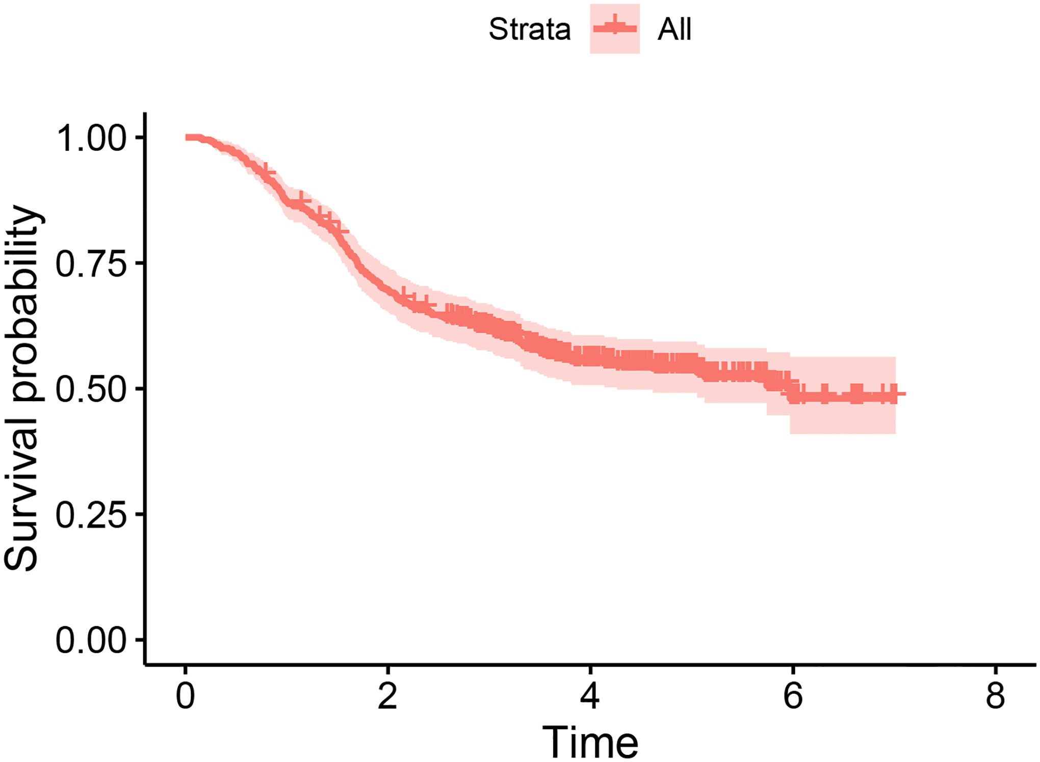
Kaplan-Meier survival curve for the cutaneous melanoma data

Figure 2 illustrates the averaged ROC curves for different models and their corresponding AUC values. It’s evident that each of the ML-based MCM models under consideration demonstrates superior predictive accuracy compared to both spline-based and logistic-based MCM models. Therefore, the comparison now focuses on distinguishing among the ML-based MCM models. Among the ML-based MCM models considered, it’s worth mentioning that each ML-based model achieves a predictive accuracy of at least 0.80, with the XGB-based MCM exhibiting the highest predictive accuracy of 0.96.

Figure 2:

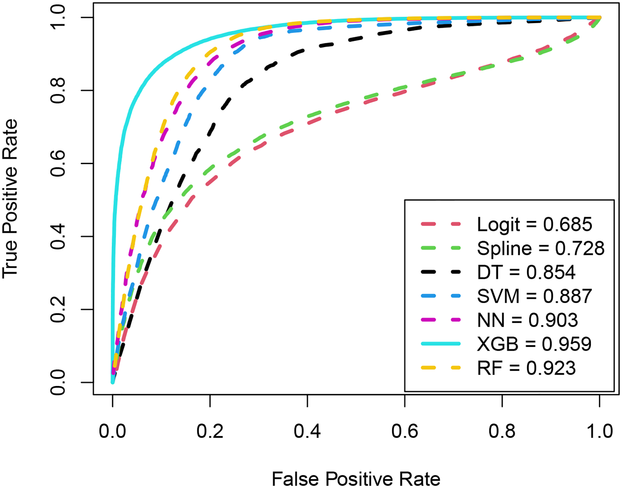
ROC curves and the corresponding AUC values under different models for the cutaneous melanoma data

Next, we examine the outcomes pertaining to the latency components of the fitted models. Table 6 provides the estimates of the latency parameters, their standard deviations (SD), and the corresponding p-values. The SDs are calculated using 100 bootstrap samples. Notably, at a significance level of 10%, Nodule Category emerges as significant across all models. It is important to highlight that the impact of Nodule Category remains consistent across all models. Given that the estimated effect associated with Nodule Category is positive, the instantaneous rate of death due to melanoma increases with an increase in Nodule Category. This observation aligns with the findings in Pal & Balakrishnan (2016). Finally, the computation times (in seconds), as presented in Table 7, indicate that the estimation results for both incidence and latency, including the bootstrap SD, can be obtained within a very reasonable timeframe.

Table 6:

Estimation results corresponding to the latency parameters for the cutaneous melanoma data

Model	Estimates				SD				$\mathit{p}$-value
	Age	Nod-Cat	Gender	Tum-Thick	Age	Nod-Cat	Gender	Tum-Thick	Age	Nod-Cat	Gender	Tum-Thick
Logit	0.089	0.229	0.034	−0.013	0.152	0.129	0.288	0.142	0.558	0.076	0.906	0.925
Spline	0.084	0.196	0.033	<-0.001	0.102	0.083	0.216	0.090	0.408	0.019	0.877	0.998
DT	0.102	0.258	−0.001	0.042	0.114	0.082	0.227	0.078	0.370	0.002	0.997	0.588
SVM	0.117	0.278	−0.002	0.048	0.091	0.085	0.201	0.069	0.201	0.001	0.991	0.491
NN	0.084	0.156	0.035	0.005	0.078	0.089	0.202	0.094	0.283	0.081	0.861	0.960
XGB	0.105	0.245	0.008	0.036	0.091	0.064	0.183	0.073	0.250	<0.001	0.965	0.624
RF	0.078	0.166	0.016	0.010	0.084	0.083	0.195	0.065	0.357	0.045	0.934	0.878

Table 7:

Computation times for different models using the cutaneous melanoma data

Model	Computing Time (in seconds)
Logit	11.564
Spline	157.621
DT	255.67
SVM	117.146
NN	549.395
XGB	272.485
RF	319.684

Figure 3 presents, for each gender type, the predicted susceptible and overall survival probabilities across different nodule categories when patients age and tumor thickness are fixed at their mean values. It is clear that patients belonging to nodule category 1 demonstrate uniformly higher survival probability (both susceptible and overall) when compared to patients belonging to nodule category 4.

Figure 3:

Predicted overall and susceptible survival probabilities (stratified by nodule category) for the mean values of patient age and tumor thickness based on the cutaneous melanoma data

6. Conclusion

Within the framework of mixture cure rate model, the conventional method for modeling incidence involves assuming a generalized linear model with a well-defined parametric link function, such as the logit link function. However, a logit-based model is restrictive in the sense that it can only capture linear effects of covariates on the probability of cure. This is the same as assuming the boundary classifying the cured and uncured subjects is linear. Consequently, if the true classification boundary is complex or non-linear, it is highly likely that logit-based models will result in biased inference on disease cure. This may also affect the inference on the survival distribution of the uncured group of patients. To circumvent these issues, we propose to model the incidence using machine learning algorithms. With the implementation of machine learning algorithms we sacrifice the easy interpretation of covariate effects on the incidence. However, to maintain the straightforward interpretation of covariate effects on the survival distribution of uncured subjects, we employ Cox’s proportional hazards structure to model latency. In contrast to utilizing a single machine learning algorithm, as commonly seen in the existing literature on mixture cure models, we deploy various machine learning algorithms and conduct a comprehensive comparison of their performances. To enhance the robustness of our comparison, we also incorporate logit-based and spline-based mixture cure models. A framework for parameter estimation is developed by employing the expectation maximization algorithm.

The findings from our simulation study indicate that when the true classification boundary is linear, the logit-based mixture cure model outperforms all other models in terms of accuracy (bias) and precision (MSE) of the estimated probabilities of being cured or uncured, along with achieving superior predictive accuracy for cure. In the simulation study, when estimating incidence and evaluating predictive accuracy for cure in scenarios with non-linear classification boundaries, either the NN-based, XGB-based, or RF-based mixture cure model demonstrates superior performance, depending on the specific parameter settings. Upon examining real cutaneous melanoma data, it becomes evident that all machine learning-based mixture cure models considered outperform both logit-based and spline-based mixture cure models in terms of predictive accuracies. Notably, for the real data, the XGB-based mixture cure model demonstrated the highest predictive accuracy at 96%.

While we have examined the effectiveness of the proposed models and methods under the influence of varying numbers of covariates with complex interaction terms, a compelling avenue for immediate future work involves extending our analyses to accommodate high-dimensional data, where the number of covariates surpasses the sample size. In this context, particular emphasis should be placed on developing methods for covariate selection and evaluating their performance under diverse parameter settings. Another possibility is to extend the entire analysis by considering the promotion time cure model (Yakovlev & Tsodikov, 1996; Pal & Aselisewine, 2023) or a suitable transformation cure model (Koutras & Milienos, 2017; Milienos, 2022) as the underlying cure model. We are actively working on these problems and anticipate presenting our findings in upcoming manuscripts.

Data availability statement

Computational codes are available at https://github.com/Aselisewine/ML-Cure-rate-model/tree/main

References

- Aselisewine W, & Pal S (2023). On the integration of decision trees with mixture cure model. Statistics in Medicine, 42(23), 4111–4127. [DOI] [PMC free article] [PubMed] [Google Scholar]
- Balakrishnan N, & Pal S (2013). Lognormal lifetimes and likelihood-based inference for flexible cure rate models based on COM-Poisson family. Computational Statistics & Data Analysis, 67, 41–67. [Google Scholar]
- Balakrishnan N, & Pal S (2015). Likelihood inference for flexible cure rate models with gamma lifetimes. Communications in Statistics - Theory and Methods, 44 (19), 4007–4048. [Google Scholar]
- Balakrishnan N, & Pal S (2016). Expectation maximization-based likelihood inference for flexible cure rate models with Weibull lifetimes. Statistical Methods in Medical Research, 25(4), 1535–1563. [DOI] [PubMed] [Google Scholar]
- Berkson J, & Gage RP (1952). Survival curve for cancer patients following treatment. Journal of the American Statistical Association, 47, 501–515. [Google Scholar]
- Boag JW (1949). Maximum likelihood estimates of the proportion of patients cured by cancer therapy. Journal of the Royal Statistical Society. Series B (Methodological), 11, 15–53. [Google Scholar]
- Cai C, Zou Y, Peng Y, & Zhang J (2012). smcure: An R-package for estimating semiparametric mixture cure models. Computer Methods and Programs in Biomedicine, 108(3), 1255–1260. [DOI] [PMC free article] [PubMed] [Google Scholar]
- Chen T, & Du P (2018). Mixture cure rate models with accelerated failures and nonparametric form of covariate effects. Journal of Nonparametric Statistics, 30(1), 216–237. [DOI] [PubMed] [Google Scholar]
- de la Cruz R, Fuentes C, & Padilla O (2022). A Bayesian mixture cure rate model for estimating short-term and long-term recidivism. Entropy, 25(1), 56. [DOI] [PMC free article] [PubMed] [Google Scholar]
- Farewell VT (1986). Mixture models in survival analysis: Are they worth the risk? Canadian Journal of Statistics, 14 (3), 257–262. [Google Scholar]
- Ibrahim JG, Chen M, & Sinha D (2001). Bayesian Survival Analysis. New York: Springer. [Google Scholar]
- Jiang C, Wang Z, & Zhao H (2019). A prediction-driven mixture cure model and its application in credit scoring. European Journal of Operational Research, 277 (1), 20–31. [Google Scholar]
- Koutras M, & Milienos F (2017). A flexible family of transformation cure rate models. Stat Med, 36 (16), 2559–2575. [DOI] [PubMed] [Google Scholar]
- Levine MN, Pritchard KI, Bramwell VH, Shepherd LE, Tu D, & Paul N (2005). Randomized trial comparing cyclophosphamide, epirubicin, and fluorouracil with cyclophosphamide, methotrexate, and fluorouracil in premenopausal women with nodepositive breast cancer: update of National Cancer Institute of Canada Clinical Trials Group Trial MA5. Journal of Clinical Oncology, 23, 5166–5170. [DOI] [PubMed] [Google Scholar]
- Li P, Peng Y, Jiang P, & Dong Q (2020). A support vector machine based semiparametric mixture cure model. Computational Statistics, 35 (3), 931–945. [Google Scholar]
- Liu X, Peng Y, Tu D, & Liang H (2012). Variable selection in semiparametric cure models based on penalized likelihood, with application to breast cancer clinical trials. Statistics in Medicine, 31 (24), 2882–2891. [DOI] [PubMed] [Google Scholar]
- López-Cheda A, Cao R, Jácome MA, & Van Keilegom I (2017). Nonparametric incidence estimation and bootstrap bandwidth selection in mixture cure models. Computational Statistics & Data Analysis, 105, 144–165. [Google Scholar]
- Maller RA, & Zhou X (1996). Survival analysis with long-term survivors. New York: John Wiley & Sons. [Google Scholar]
- McLachlan GJ, & Krishnan T (2007). The EM algorithm and extensions (Vol. 382). John Wiley & Sons. [Google Scholar]
- Milienos FS (2022). On a reparameterization of a flexible family of cure models. Stat Med, 41 (21), 4091–4111. [DOI] [PubMed] [Google Scholar]
- Pal S (2021). A simplified stochastic EM algorithm for cure rate model with negative binomial competing risks: an application to breast cancer data. Statistics in Medicine, 40 (28), 6387–6409. [DOI] [PubMed] [Google Scholar]
- Pal S, & Aselisewine W (2023). A semiparametric promotion time cure model with support vector machine. Annals of Applied Statistics, 17 (3), 2680–2699. [Google Scholar]
- Pal S, & Balakrishnan N (2016). Destructive negative binomial cure rate model and EM-based likelihood inference under Weibull lifetime. Statistics & Probability Letters, 116, 9–20. [Google Scholar]
- Pal S, & Balakrishnan N (2017a). Likelihood inference for COM-Poisson cure rate model with interval-censored data and Weibull lifetimes. Statistical Methods in Medical Research, 26 (5), 2093–2113. [DOI] [PubMed] [Google Scholar]
- Pal S, & Balakrishnan N (2017b). Likelihood inference for the destructive exponentially weighted Poisson cure rate model with Weibull lifetime and an application to melanoma data. Computational Statistics, 32 (2), 429–449. [Google Scholar]
- Pal S, Peng Y, & Aselisewine W (2023). A new approach to modeling the cure rate in the presence of interval censored data. Computational Statistics, DOI: 10.1007/s00180-023-01389-7. [DOI] [PMC free article] [PubMed] [Google Scholar]
- Pal S, Peng Y, Aselisewine W, & Barui S (2023). A support vector machine-based cure rate model for interval censored data. Statistical Methods in Medical Research, 32 (12), 2405–2422. [DOI] [PMC free article] [PubMed] [Google Scholar]
- Pal S, & Roy S (2021). On the estimation of destructive cure rate model: a new study with exponentially weighted Poisson competing risks. Statistica Neerlandica, 75 (3), 324–342. [Google Scholar]
- Pal S, & Roy S (2022). A new non-linear conjugate gradient algorithm for destructive cure rate model and a simulation study: illustration with negative binomial competing risks. Communications in Statistics - Simulation and Computation, 51 (11), 6866–6880. [DOI] [PMC free article] [PubMed] [Google Scholar]
- Pal S, & Roy S (2023). On the parameter estimation of Box-Cox transformation cure model. Statistics in Medicine, 42 (15), 2600–2618. [DOI] [PubMed] [Google Scholar]
- Peng Y (2003). Fitting semiparametric cure models. Computational Statistics & Data Analysis, 41 (3–4), 481–490. [Google Scholar]
- Peng Y, & Dear KB (2000). A nonparametric mixture model for cure rate estimation. Biometrics, 56 (1), 237–243. [DOI] [PubMed] [Google Scholar]
- Peng Y, & Yu B (2021). Cure Models: Methods, Applications and Implementation. Chapman and Hall/CRC. [Google Scholar]
- Platt J, et al. (1999). Probabilistic outputs for support vector machines and comparisons to regularized likelihood methods. Advances in Large Margin Classifiers, 10 (3), 61–74. [Google Scholar]
- Sy JP, & Taylor JM (2000). Estimation in a Cox proportional hazards cure model. Biometrics, 56, 227–236. [DOI] [PubMed] [Google Scholar]
- Tong EN, Mues C, & Thomas LC (2012). Mixture cure models in credit scoring: If and when borrowers default. European Journal of Operational Research, 218 (1), 132–139. [Google Scholar]
- Treszoks J, & Pal S (2022). A destructive shifted Poisson cure model for interval censored data and an efficient estimation algorithm. Communications in Statistics-Simulation and Computation, DOI: 10.1080/03610918.2022.2067876. [DOI] [Google Scholar]
- Treszoks J, & Pal S (2023). On the estimation of interval censored destructive negative binomial cure model. Statistics in Medicine, 42 (28), 5113–5134. [DOI] [PMC free article] [PubMed] [Google Scholar]
- Treszoks J, & Pal S (2024). Likelihood inference for unified transformation cure model with interval censored data. Computational Statistics, DOI: 10.1007/s00180-024-01480-7. [DOI] [Google Scholar]
- Xie Y, & Yu Z (2021a). Mixture cure rate models with neural network estimated nonparametric components. Computational Statistics, 36, 2467–2489. [DOI] [PubMed] [Google Scholar]
- Xie Y, & Yu Z (2021b). Promotion time cure rate model with a neural network estimated non-parametric component. Statistics in Medicine, 40(15), 3516–3532. [DOI] [PubMed] [Google Scholar]
- Xu J, & Peng Y (2014). Nonparametric cure rate estimation with covariates. Canadian Journal of Statistics, 42 (1), 1–17. [Google Scholar]
- Yakovlev AY, & Tsodikov AD (1996). Stochastic models of tumor latency and their biostatistical applications. Singapore: World Scientific. [Google Scholar]
- Zhang J, & Peng Y (2007). An alternative estimation method for the accelerated failure time frailty model. Computational Statistics & Data Analysis, 51, 4413–4423. [Google Scholar]
Associated Data
This section collects any data citations, data availability statements, or supplementary materials included in this article.