

Abstract
Despite its importance, the fine structure of the human brain is understudied. Presented here is a computationally intensive reconstruction of the ultrastructure of a cubic millimeter of human temporal cortex, surgically removed to gain access to an underlying epileptic focus. It contains ~57,000 cells, ~230 millimeters of blood vessels, ~150 million synapses, and comprises 1.4 petabytes. We share tools online to render, analyze and proofread these data and found that glia outnumber neurons 2:1, oligodendrocytes were the most common cell, deep layer excitatory neurons could be classified based on dendritic orientation, and among thousands of weak connections to each neuron, there exist rare powerful axonal inputs of up to ~50 synapses. Additional insights will likely emerge from further study of this resource.
Introduction:
While the functions carried out by most of the vital organs in humans are not remarkably different when compared to other animals, the functions carried out by the human brain clearly separate us from the rest of life on the planet. Detailed knowledge, however, concerning the synaptic circuitry underlying human brain function is lacking. Connectomic imaging approaches are now available to render neural circuits of sufficiently large volume and high resolution to dissect the connectivity at the level of individual neurons and their synaptic connections but over a scale comprising thousands of neurons. Generating such a data set was the goal of this project.
Rationale:
One critical barrier to obtaining human neural circuits has been the access to high quality human brain tissue. Organ biopsies provide valuable information in many human organ systems, but biopsies are rarely done in the brain except to examine or excise neoplastic masses, and hence, most of them are problematic for the investigation of normal human brain structure. One attempt has been to use brain organoids made from human cells but at present they do not approximate brain tissue architectonics (e.g., cortical layers are not present). A direct approach would be to map cells and circuits from human specimens made available owing to neurosurgical interventions for neurological conditions where pieces of the cortex are discarded, because they obstruct access to a pathological site. We posited the human brain tissue that is a byproduct of neurosurgical procedures can be leveraged to understand normal, and ultimately disordered human neural circuits.
Results:
Here we describe such a sample of human temporal cortex, a cubic millimeter in volume, that extends through all cortical layers, obtained during surgery to gain access to an underlying hippocampal lesion from a patient with epilepsy. We imaged this sample by high-throughput serial section electron microscopy, generating a petascale dataset that was analyzed with novel tools and computationally intensive methods. The resulting dataset provided reconstructions of thousands of neurons, more than a hundred million synaptic connections, as well as all the other tissue elements that comprise human brain matter including glial cells, the blood vasculature, and myelin. Because the dataset is large and incompletely scrutinized, to aid in its analysis we share all of the data online and provide tools for analysis and proofreading. We provide two vignettes of new insights that emerged from our initial analyses: a new class of directionally oriented neurons in deep layers, and the presence of very powerful rare muti-synaptic connections between neurons throughout the sample.
Conclusion:
This work provides evidence of the feasibility of human connectomic approaches to visualize and ultimately gain insight into the physical underpinnings of normal and disordered human brain function. It is hoped that this endeavor will be aided by providing free access to all the data and relevant tools.
One-Sentence Summary:
A millimeter-scale fragment of human cerebral cortex imaged and segmented at nanoscale resolution and made available online.
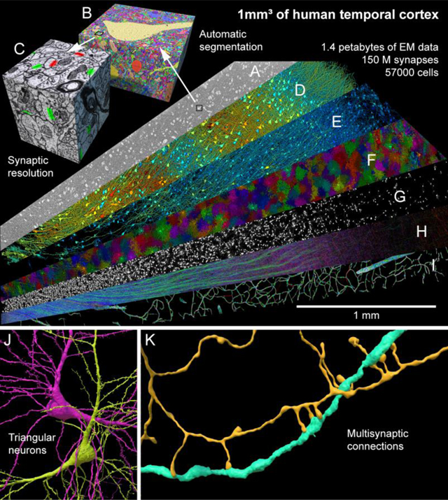
Graphical Abstract
The shared H01 dataset. A range of histological features in a cubic millimeter of human brain were rendered including neuropil (A) and its segmentation (B) at nanometer resolution, annotated synapses (C), excitatory neurons (D), inhibitory neurons (E), astrocytes (F), oligodendrocytes (G), myelin (H), and blood vessels (I). A new way of dividing layer 6 neurons (J) and powerful multisynaptic inputs (K) were identified.
Introduction
The human brain is a vastly complicated tissue, and to date, little is known about its cellular microstructure, and in particular, its synaptic circuits. These circuits, when disrupted, likely underlie incurable disorders of human brain function. Technologies such as diffusion MRI tract tracing (1), high resolution MR (2), fMRI (3) and others (see reviews in 4, 5) have improved our knowledge of the structure and function of the human brain at and below millimeter resolution. However, to identify the structure of neural networks at the synaptic level requires orders of magnitude higher resolution using light or electron microscopy (EM). Light microscopical approaches to see neural networks have been successful in tracing full connectivities in the peripheral nervous system where the density of axons is low (6, 7). Light-based methods in the central nervous system are advancing rapidly (8–16), however for dense neural networks the most successful approaches in the brain have used volume electron microscopy, where reconstruction of every cellular element and synapse is possible, owing to the extremely high spatial resolution afforded by the short wavelength of electrons (17–25). Because of automation and rapid imaging modalities, serial electron microscopy (SEM) can now scale to image cubic millimeter volumes at nanometer resolution. Our aim was to use these approaches in a human brain tissue sample.
High quality human brain tissue specimens are available from neurosurgical interventions in living patients where part of the cortex has to be removed because it obstructs access to a pathological region. Here we describe such a sample, a rapidly preserved (see Methods) 170 micrometer thick slab of human cortex from the anterior part of the middle temporal gyrus, with a total volume of just over one cubic millimeter that was removed to gain access to an epileptic focus in the underlying hippocampus. An important caveat related to human surgical samples is that they originate in patients with pathologies of the nervous system, such as epilepsy, tumors, or neurodegenerative diseases. In this case, we cannot exclude the possibility that long-term epilepsy, or its pharmacological treatment, had subtle effects on the nanometer-scale structure of the sample. However, at least by light microscopy-based neuropathological examination, the sample was deemed normal, lacking for example, the band of aggregated neurons noted in the outer part of layer 2 when hippocampal sclerosis associated with epilepsy extends into the adjacent temporal lobe (26).
This is, to our knowledge, the largest volume of human cortex at electron-microscopic resolution produced and the first EM dataset to exceed a petabyte in size. We sought to reconstruct a human sample spanning all six layers of cortex, approximately 3 millimeters from layer one to the white matter. Given the throughput limits of serial section electron microscopy, this constrained the total thickness of the reconstructed sample. However, because the sample is oriented perpendicular to the pia and follows the fanned-out directions of the principal axons and dendrites of pyramidal neurons, many of these could be traced across cortical layers. The acquisition, computational alignment, automated 3d segmentation, and automated synaptic annotation of digital human brain tissue at this large scale, and this fine resolution, enables not only access to neuronal circuitry comprising thousands of neurons and millions of synapses, but also provides a clear view of all the other tissue elements that comprise human brain matter including the glial cells, blood vasculature, and the relations between various cell types. A wide range of questions related to human brain biology are thus open to scrutiny from a single sample. To aid in its analysis we are sharing all of the data, and tools to analyze it, online.
Methods
Reconstruction Pipeline
The sample we analyzed is from excess tissue of the anterior middle temporal gyrus resected as part of treatment for drug-resistant epilepsy and subjected to rapid immersion fixation that provided excellent preservation of ultrastructure (see Supp. Materials and Methods). The tissue was further preserved and stained with osmium, and other heavy metals using a ROTO staining protocol (27). The sample was then embedded in a resin, trimmed, and 5019 sections were collected at an average thickness of 33.9 nm (with 92.5% of the sections between 30 and 33 nm; see Supp. Materials and Methods for details) using an automatic tape-collecting ultramicrotome (ATUM) (28) for a total sample thickness of 0.170 millimeters. Each section was imaged using a multibeam scanning electron microscope at 4 × 4 nm2 resolution (fig. 1A). Because cutting these sections caused compression by 28% in the cutting direction, we adjusted for this by correcting the pixel size to 5.55 × 4 nm, giving a total imaged volume of 1.05 mm3 (uncompressed tissue). The raw data size was up to 350 GB per section, 1.8 petabytes in total. While the microscope was acquiring images, a custom-built workflow manager assessed each tile for quality and flagged problems. The total throughput of image acquisition ranged from 125 to 190 million (M) pixels per second. The majority of the data was acquired at 190 M pixels per second (see table S1 for details). The total imaging time for the 1 mm3 sample was 326 days.
Figure 1: The H01 dataset, image acquisition and alignment.

(A) A fresh human surgical cerebral cortex sample was rapidly preserved, stained, embedded in resin, sectioned at ~33 nm, collected on tape and imaged using the ATUM-mSEM method. The Zeiss mSEM electron microscope uses 61 beams that image a hexagonal area of about ~10,000 μm2 simultaneously, which allows for large areas to be imaged rapidly. For each section, all the resulting tiles are then stitched together (left; this section is about 4 mm2 in area and was imaged with 4 × 4 nm2 pixels - see image of synapse at right). Given the necessity of some overlap between the stitched tiles, this single section required the collection of more than 300 GB of data. (B) Fine-scale alignment with optical flow. Left: An XZ cross-section of the initial coarsely aligned subvolume exhibits drift and jitter. Center: Two adjacent XY sections z (green) and z-1 are overlaid to illustrate their misalignment. Image patch-based cross-correlation computes an XY flow field between them. Red and blue intensities, which indicate the respective horizontal and vertical flow components are used to warp one of the sections, improving their alignment (relax and warp overlay). Right: XZ view of the same subvolume with flow realignment applied.
The raw acquired image tiles were first stitched together and coarsely aligned by using microscope stage coordinates, semi-automated feature correspondences, and image patch cross-correlations to relax an elastic triangular mesh of each tile and each section (fig. 1B, left) (29). A fine-scale refining alignment based on optical flow between neighboring sections removed remaining drift and jitter from the volume (fig. 1B, center and right). From a total of 247 M tiles (1.8 PB), 196 M tiles containing cortex were stitched together and aligned, creating a unified ~1.4 PB human cerebral cortex image volume, approximately triangular in shape (fig. 1A).
Three dimensional reconstruction of the structure of nearly every cell and process in the aligned volume proceeded by the use of a multi-resolution Flood-Filling Network (FFN) to segment the image data (30), producing base segments, which are fragments of whole objects (fig. 2A). These base segments were then agglomerated via FFN resegmentation (see Supp. Materials and Methods) to produce more complete reconstructed cells (fig. 2B). Occasional agglomeration errors produced mergers between nearby objects, such as a passing axon and dendrite (fig. 2C, left). We used subcompartment predictions (31) to distinguish the two merged objects, by classifying all skeleton nodes within each cell as either axon, dendrite, astrocyte, soma, cilium, or axon initial segment (fig. 2C, center), which allowed an automated cut to be made at the site of merge errors (fig. 2C, right). These automated corrections removed nearly all split and merge errors, but some errors remain, since there is a trade-off between removing split errors and adding merge errors. Two different agglomerations are therefore made available: one which favors fewer breaks (and hence longer processes) but with a higher number of incorrect mergers, named ‘c2’, and one that is more conservative and has shorter fragments but fewer merge errors, named ‘c3’. All analyses described subsequently are based on the c3 agglomeration.
Figure 2: Segmentation, split correction, merge error correction via neuronal sub-compartment classification and synapse prediction.

(A) Example of sequential segmentation with a Flood Filling Network (FFN). Objects are filled sequentially from seed locations until the 3D volume is segmented completely. (B) FFN agglomeration. Left: Site between two adjacent base segments (white box in 2D, black box in 3D below) is a candidate agglomeration location. Center: FFN segmentation is seeded from points A and B independently. Right: If the resulting A and B segmentations are mutually consistent, the object pair is merged (below). (C) Subcompartment prediction and merge error correction (link). Left: a single reconstructed object with a merge error where axon and dendrite cross near each other. The object is converted to a reduced skeleton representation (blue). Middle: fields of view around a subset of skeleton nodes are input to a subcompartment classification model. Red nodes: predicted dendrite; blue nodes: predicted axon. The inconsistency in subcompartment predictions is detected, and the agglomeration graph is cut at the location that maximally improves subcompartment consistency. Right: the separated axon and dendrite after applying the suggested cut. (D) Synapse detection and classification. Top: XY cross-section of EM image input to synapse detection model (left), and the resulting presynaptic (magenta) and postsynaptic (green) prediction masks (right). Bottom: cross-section of EM image and presynaptic (left red, right blue) and postsynaptic (green) object segmentation inputs to excitatory versus inhibitory classification model. Right: 3D render of a dendrite with predicted incoming excitatory (yellow) and inhibitory (blue) synaptic sites.
To compare the frequency of split and merge errors between the c2 and c3 agglomerations, we proofread 104 randomly-selected neurons, correcting all split and merge errors of axons, dendrites and somata. We found that, on average, the c3 agglomeration required 1.6-fold less correction of merge errors (257 vs. 400 merge correction operations per cell, p < 10−7) but 2.1-fold more correction of split errors (504 vs. 238 split correction operations per cell, p < 10−10) when compared to the c2 agglomeration, consistent with the c3 agglomeration being more conservative (table S2). This analysis only included breaks in dendritic branches, and not the disconnection of dendritic spines, because manual proofreading of the hundreds of thousands of spines on these 104 cells was infeasible. Notably, proofreading 1550 spines on the dendritic tree of a layer 2 pyramidal neuron did not reveal a substantial difference in split errors detaching dendritic spines, with 32.2% of its spines detached from dendritic shafts in the c2 segmentation, vs. 33.7% in the c3 segmentation. Split errors were not uniformly distributed across the H01 volume, as shown by mapping the tendency of segments in the c3 agglomeration to traverse consecutive z-layers (see Supp. Materials and Methods for details and fig. S1). Merge errors in the base segmentation itself were rare, being observed in only 13 base segments out of 365,404 base segments comprising the proofread neurons (0.0036%).
To be able to analyze the connectivity between neurons in this dataset, identifying synapses was necessary. As shown in fig. 2D, we used machine learning tools to train automated synapse classifiers to identify the pre- and postsynaptic component of each synapse and whether the presynaptic terminal was excitatory or inhibitory (see Supp. Materials and Methods). Proofreading a selection of axons covering all cortical layers showed that the number of missed synapses (i.e., false negatives) for excitatory and inhibitory synapses was 11% and 35%, respectively. The false discovery rate for excitatory and inhibitory synapses was 3.2% and 2.7%, respectively (table S3). Automated classification of each synapse as excitatory or inhibitory was based on the appearance of each individual synapse and whether its postsynaptic structure was a dendritic spine or not, as well as the whether the presynaptic neuron was an excitatory or inhibitory type, for those neurons where the soma was in the volume. In total, we found 149,871,669 synapses in the volume. Analyzing the post-synaptic component of 133,704,881 of these (see Supp. Materials and Methods), we found as expected, a high percentage of these synapses located on dendrites (99.4%), with far fewer innervating the AIS (0.197%) or somata (0.394%). 111,272,315 synapses were classified as excitatory and 38,599,354 as inhibitory, with excitatory and inhibitory synapses classified correctly 86.89% and 84.98% of the time, respectively. Adjusting for the measured false discovery, false negative and excitatory/inhibitory mis-classification rates, we estimate that the H01 volume contains a total of 111.6 M (61.2%) excitatory synapses and 70.7 M (38.8%) inhibitory synapses.
Tools for Cell Reconstruction and Circuit Exploration
While some analyses of the data are not significantly impacted by the agglomeration split and merge errors described above, other analyses, particularly those at the level of neuronal circuits, require correction of these agglomeration errors by proofreading. Due to the large number of neuronal structures, it is infeasible for a single lab to proofread the entire dataset manually. To facilitate scientific studies that require correction of agglomeration errors by proofreading, we provide a collaborative proofreading platform for H01 built upon the CAVE (Connectome Annotation and Versioning Engine) infrastructure (32). This tool is web-based and tightly integrated with the Neuroglancer viewer. Proofreaders can interactively update the segmentation by correcting merge and split errors. All proofreaders have access to the most up-to-date segmentation at all times to avoid redundant edits by multiple community members. We selected the c3 agglomeration as a starting point for the collaborative proofreading process. Anyone can apply to become a proofreader (see platform), and proofreaders may download data relating to the cells that they have proofread for subsequent analyses (see tutorials). The most recent version of the proofread volume is always available to browse by any interested researcher without applying to be a proofreader.
VAST (33) is a versatile free software tool to view, segment and annotate large voxel datasets. In contrast to the CAVE system described above that focuses mainly on correction of split and merge errors of the agglomerated segmentation, VAST can be used to generate novel ground-truth segmentations of objects of interest (e.g., vasculature or organelles) by manual voxel painting and to create annotated binary skeletons for quantitative analysis (e.g., volume or length measurements). VAST can also be used to agglomerate c2 or c3 segments locally. To make the H01 image data available in VAST, we extended the program to read data directly from the Neuroglancer-compatible online storage. Results from VAST can be exported in various formats for analysis and visualization. VAST also includes an API which allows for script-based automation through Matlab. VAST was used for several results in this paper, including the manual labeling and classification of all cell bodies described below.
For analysis, various databases have been made available to enable specific queries about the cellular and synaptic data. However, these are not integrated with the neuroglancer platform, and do not support more complex queries at the neuronal network level. To address this, we developed a standalone program, CREST (Connectome Reconstruction and Exploration Simple Tool). CREST can be used to identify and explore the connections of cells based on a number of those cells’ features, including the numbers of synaptic inputs or outputs of a given strength (see strong synaptic connections described below). CREST can also be used to explore and graph chains of synaptically connected neurons, finding both how a neuron’s postsynaptic influence diverges across multiple generations of downstream neurons and how presynaptic influences converge from multiple generations of upstream neurons. It should be noted that paths identified in this way require manual verification given the presence of agglomeration merge errors, and - to a lesser extent - synapse false positives. Verified paths of interest can be saved locally, along with the schematic view of the path, for later re-viewing via the CREST tool. Finally, CREST also features a proofreading tool, which allows cells to be proofread and each version of a cell saved locally. Detailed user instructions are available from the CREST homepage and here.
Results
Cellular and Synaptic Organization
The entire segmented volume (fig. 3), including the synaptic and subcompartment annotations are available for exploration within the neuroglancer platform. Instructions on how to explore the various data overlays, modify their appearance and navigate the H01 dataset are available here.
Figure 3. The segmented H01 volume.

Left: Oblique view of the H01 dataset following all automatic segmentation steps, trimmed to the fully imaged volume, and stretched to compensate for section compression from ultrathin sectioning. The C3 auto-segmentation is overlaid in random color. Right: Cut-out of the dataset at the location of the red rectangle in G, showing a cross-section of the aligned image stack. The pink lines show where the two sectioning series join (‘Phase 1’ and ‘Phase 2’).
The H01 resource is divisible into many subcategories. Based on skeleton node classifications and manual annotations, and excluding extracellular spaces, myelinated axon sheaths and tissue artifacts (see Supp. Materials and Methods), the neuropil by volume is comprised of unmyelinated axons (~40.2%), dendrites (~25.8%), glial processes (~15.5%), somata (~9.4%), myelinated axons excluding their sheaths (~7.5%), collapsed blood vessels (~1.5%), axon initial segments (~0.07%), and cilia (~0.03%; see also table S4 for breakdown by cortical layer). In addition to these well known categories, we found a number of UCOs (unidentified cortical objects) that accounted for very little volume (fig. S2).
We analyzed all the cells with nuclei in the sample (fig. 4), manually identifying and quantifying them (table S5, table S6). There were 49,080 neurons and glia (fig. 4A) and 8100 blood vessel-related cells (fig. 4B; 57,180 cells total). Glia outnumber neurons 2:1 (32,315 versus 16,087). Of the neurons, 65.5% were spiny (10,531, of which 8,803 had a pyramidal shape), 29.1% were non-spiny (4,688) and classified as interneurons, and 5.4% (868) did not easily fit into this binary categorization mostly because their somata were not fully in the volume. There were also some unusual neurons that were difficult to classify, samples of which are shown in fig. S3. Overall, the density of neurons was ~16,000/mm3, approximately one third lower than previously estimated from light microscopy of human temporal cortex (34), and nearly 10-fold lower than in association cortex of the mouse (35–37).
Figure 4: Distribution of cells, blood vessels and myelin in the sample.

White lines indicate layer boundaries based on cell clustering. (A) All 49,080 cell bodies of neurons and glia in the sample, colored by soma volume. (B) Blood vessels and the nuclei of the 8,136 associated cells (link). Inset shows a magnified view of the location of the individual cell types. (C) Spiny neurons (n=10531; putatively excitatory), colored by soma volume. (D) Interneurons (n=4688; few spines, putatively inhibitory), colored by soma volume. (E) Astrocytes (n=5474) mostly tile but in some cases, arbors of nearby astrocytes interdigitate. (F) Most of the oligodendrocytes (n=20139) in the volume. Note clustering along large blood vessels, especially in white matter. (G) Cell bodies (n=6702) of microglia and oligodendrocyte precursor cells (OPCs). (H) Myelinated axons in the volume, color-coded by topological orientation. Most axons in white matter run in the perpendicular direction. Thick axon bundles run between white matter and cortex in the radial direction. In layer 1, a set of large-caliber myelinated axons runs tangentially through our slice, parallel to the pia. In layers 3–6 many myelinated axons also run in diagonal (tangential/perpendicular) directions. Images and scale bar as in sections (with ultrathin sectioning compression).
The cells showed macroscopic organization: cortical layers were evident by cell soma volume (fig. 4A). To find an objective layering boundary criterion, we used cell soma size and clustering density, generating a 6-layered cortex and white matter (see Supp. Materials and Methods and fig. S4). The fiducial lines in each panel of fig. 4are based on these layers (named in fig. 4A). There were fewer cells with large cell bodies in the white matter and cortical layer 1 because these regions were populated mainly by glial cells whose cell body sizes were smaller than neurons (fig. 4A, blue). The largest cells (red) were mostly in a broad deep infragranular band corresponding to layer 5 and a supragranular one corresponding to layer 3, as expected (38). The 3D shape of cells plus their electron microscopical appearances allowed their classification into types. The largest cell somata belonged to spiny pyramidal neurons, with variation in soma size across the cortical layers (fig. 4C). Non-pyramidal neurons were much less spiny, had smaller cell body sizes and, as a group, were not obviously arranged into layers (fig. 4D).
The glial cells did show differences between layers (fig. 4E, F and G). The compact and complicated arbors of protoplasmic astrocytes were densely tiled in layers 2–6 as described previously (39–41). However, in the more superficial parts of layer 1, they were often more intermingled, had a higher density, and were smaller in size (fig. 4E, fig. S5A,B,E). Fibrous astrocytes in the white matter were more elongated than the astrocytes that occupied the cortical layers.
Two other kinds of glia, microglia and oligodendrocyte precursor cells (OPCs), had almost even density across all layers but showed affinity for vasculature (fig. S5C), while astrocyte cell bodies did not (42). Due to the similar morphologies of OPCs and microglia, machine learning was used to distinguish these types (see Supp. Materials and Methods and 43), with 2,517 cells predicted as microglia, 1,626 as OPCs, and 2,102 that were unclassified (fig. 4G; fig. S6).
Another type of glia, oligodendrocytes (n = 20,139), were distributed according to a gradient, with the lowest density in the upper layers and highest density in the white matter, as expected, given their role in myelin formation (fig. 2F; fig. S5E). Like microglia and OPCs, oligodendrocytes showed affinity for blood vessels (fig. S5C). Perivascular oligodendrocytes formed lines along radially-oriented blood vessels in the white matter, and to a lesser degree elsewhere in the volume (fig. S5D). Myelin, a product of oligodendrocytes, followed the oligodendrocyte density gradient, with the highest density in the white matter and the lowest in layer 2 (fig. 4H; table S4). Significant numbers of myelinated axons ran radially between the white matter and superficial layers (fig. 4H, green) and horizontally within layers in two orthogonal axes (fig. 4H, red and blue). The myelin in the white matter ran primarily orthogonal to the plane of the section (fig. 4H, blue; see also fig. S7). These orientations provide signals that affect diffusion tensor measurements made in the human brain in vivo (44).
The reconstructed blood vessels (~230 mm in length) did not show much evidence of layer-specific behavior but had a lower density in the white matter, presumably for energetic reasons (45) and in the regions surrounding large vessels (fig. 4B). The vasculature was lined by 4,604 endothelial cells (green, ~20 per mm of vasculature) and a more heterogeneous group of 3,549 pericytes and other perivascular cell types (blue, ~15 per mm of vasculature) also within the basement membrane, but displaced slightly further from the lumen (fig. 4B). Bloodless bridges (n=74), composed of basement membrane and pericytes but lacking endothelial cells and a lumen (46), (47), (48) connected different capillaries in the dataset (red in fig. 4B).
From a functional standpoint, a critical component of brain tissue is its synapses. Using a U-Net classifier ~150M synapses were identified and divided into two categories, excitatory and inhibitory (see Supp. Materials and Methods). The density of the ~111M excitatory synapses was highest in layers 1 and 3 (fig. 5A), whereas the ~39M inhibitory synapses peaked in density in layer 1 (fig. 5B). The percentage of excitatory synapses of total E/(E+I) was broadly similar across layers, being slightly lower in layer 1 (fig. 5C), as previously reported (34). The identification of all synapses and their assignment to specific pre- and post-synaptic partners allowed the rendering of excitatory and inhibitory input to each pyramidal cell (fig. 5D) and interneuron (fig. 5E) in the c3 agglomeration. For each of the cortical layers 2 to 6, a greater proportion of synaptic inputs to pyramidal neurons were excitatory compared to the inputs to non-spiny interneurons (p < 10−8 for each layer, see fig. 5F and table S7).
Figure 5: Synapse distributions.

(A) Volumetric density of excitatory (E) synapses. (B) Volumetric density of inhibitory (I) synapses. (C) Percentage of E synapses in different layers (E/E+I * 100%). Lowest values are purple, highest values are yellow. (D) Representative pyramidal neuron; note that synapses on the AIS, cell body and proximal dendrites were largely I (blue), whereas in the spiny dendritic regions there were more E synapses (orange) than I. Of the three compartments, the density of synapses is highest along the AIS and strikingly sparse on the soma. (E) Representative interneuron, with E (orange) and I (blue) synapses distributed more uniformly along dendrites and the cell soma and few if any synapses on the AIS. (F) Violin plot showing balance of E and I synapses (E/E+I) established onto interneurons (blue) and pyramidal neurons (orange), analyzed separately by the cortical layer location of neurons’ cell bodies. Gray bars indicate 1 SD from the mean (blue line).
To see what kinds of biological insights might be made from the use of this resource, we then examined two phenomena that we came across while looking at the image data. One of these concerned an unexpected cell type and the other an unexpected kind of connectivity. These two vignettes are described below.
New morphological subcategories of layer 6 triangular neurons
The deepest layer of the cerebral cortex is not well characterized compared to more superficial layers (49), in part because it contains a greater diversity of cell types, especially in primates (50). This resource provides a large set of deep layer neurons and can therefore potentially be used to better characterize these cell types. As a test of this idea, we looked at the so-called “triangular” or “compass” cells that reside in layer 6, but are not well understood (49, 51–53). These spiny neurons are characterized by an apical-going dendrite, however, unlike pyramidal neurons, they each have one especially large basal dendrite, rather than a more uniform skirt of basal dendrites. We identified all the triangular neurons in the H01 volume (fig. 6A), most of which resided in layers 5 and 6 (n = 876), comprising approximately one third of the spiny neurons in these layers.
Figure 6: Two mirror symmetrical subgroups of deep layer triangular neurons.

(A) Location of neurons with both one large apical and one large basal dendrite; most are found in layers 5 and 6. Color represents cell soma size, as in fig. 4A. (B) Distribution of directions of the basal dendrites of triangular neurons, where the direction is the angle between the radial direction and the basal dendrite direction. (C) Side view of the neurons with apical dendrites pointing either forward in the z-stack (magenta) or in the reverse direction (light green). Notice, as shown in panel B, that many of the magenta or light green neurons project their large basal dendrite at very similar angles. (D) Example of two triangular neurons with basal dendrites pointing in opposite directions showing the mirror symmetry of these two subgroups. (E) The histogram of basal dendrite angles around the radial direction shows a clear bimodal distribution with peaks at 90 and 270 degrees representing the light green and magenta groups respectively. (F) Polar plot of the data in B and E. Light green: 339 triangular cells with basal dendrite pointing towards section 0; magenta: 347 triangular cells with basal dendrite pointing towards section 5292; light and dark gray: 106 and 80 triangular cells with basal dendrite pointing sideways in the cutting plane. 4 triangular cells were excluded because their basal dendrite pointed away from the white matter. (G) Explanation of the directional color coding in this figure. (H, I, J) Anatomical clustering among members of the two subgroups, to exclude edge bias we limited analysis to cells with cell bodies centered in the middle half of the image stack (sections 1323 – 3970; n=431, 218 forward, 213 reverse). (K) The neurons shown in I are significantly more likely adjacent to a neuron whose large basal dendrite points in the same direction as they do (Fisher’s exact test, p=0.005).
The large basal dendrites of triangular neurons emerged from the cell somata at various angles (hence the name “compass cell”), ranging from 180 degrees from the apical dendrite, i.e., towards the white matter, to ~90 degrees from the apical dendrite. The mean orientation was ~126 degrees (fig. 6B). Looking at these cells suggested that many of them fell into two categories along the anterior/posterior axis: those whose basal dendrite projected towards section 1 (in the “reverse-going” direction), and those whose basal dendrite projected in the opposite (“forward-going”) direction, towards section 5292 (green and magenta cells, respectively; fig. 6C, D, see video). By taking into account the curvature of the layers, we obtained a locally-calculated average apical dendrite direction (i.e. in the ‘radial direction’ towards the pia, see fig. S8). Using this data and the orientation of the basal dendrite, we found that the majority (~77.5%) of the triangular cells were either clearly forward (n = 347) or reverse going (n = 339) forming a bimodal distribution, while the rest had basal dendrites that were more tangential (n = 186; 4 cells were outliers with basal dendrites pointing towards radial direction) (fig. 6 E, F, G). The axis formed by these basal dendrites is the main axis of the myelinated axons in the subjacent white matter, which, based on the information available, is the anterior/posterior axis of the temporal lobe.
The fact that the basal dendrites, on average, pointed slightly towards the white matter meant that the two sets of basal dendrites were not parallel to each other. Rather, each subgroup had basal dendrites at mirror symmetrical angles (fig. 6C, D). Interestingly we found other mirror symmetrical features, such as the relative absence of branches on the upper side of the basal dendrite and scarcity of apical dendrite branches pointing in the same direction as the basal dendrite (see for example, fig. 6D).
When we rendered the two subgroups of neurons (forward-going or reverse-going) it appeared that they were not uniformly distributed. To avoid identification bias at the border of the image stack, we included only neurons with cell bodies located in the middle half of the volume (centered in sections 1323–3970; n=431; fig. 6H, I, J). We then analyzed the nearest neighbor triangular cell to each of these neurons, and found that its basal dendrite pointed in the same direction as the basal dendrite of its nearest neighbor more often than expected by chance, showing statistically significant clustering (fig. 6K; Fisher’s exact test, p=0.005). This indicates that indeed, these cells cluster to some degree. Patchiness of axonal projections to layer 6 has been seen with anterograde labeling experiments in humans (54). What the function of this bimodal distribution of triangular cell basal dendrite directions signifies remains unknown.
Multi-synaptic connections between axons and specific post-synaptic partners
Previous work showed that occasionally axons in rodent cerebral cortex establish multiple synapses on the same postsynaptic cell (25, 55). We sought to examine whether the same phenomenon exists in human cerebral cortex. CREST was used to systematically identify strong connections, where a single axon established multiple synapses on the same postsynaptic cell. Many examples of this phenomenon were found. These included excitatory and inhibitory axons that innervated excitatory and inhibitory postsynaptic dendrites in any combination (fig. 7A, B, C, D). These strong connections were rare. For nearly all cells, the histogram of the number of synapses per axonal input showed a rapid fall-off from the most common occurrence where an axon established one synapse with a target cell (96.49%). Two synapse contacts occurred uncommonly (2.99%), even fewer three synapse contacts were observed (0.35%) and connections with four or more synapses occurred rarely (0.092%; see table S8 for counts of inputs to all neurons). Despite the overall rarity of strong connections however, we found that 39% of the 2743 neurons that were well innervated in the volume (i.e. that had at least 3000 synapses onto their dendrites) had at least one input that had 7 or more synapses, raising the possibility that rare powerful axonal inputs are a general characteristic of neuronal innervation in human cerebral cortex. These analyses excluded chandelier cell axons innervating axon initial segments (AIS) which are well-known to commonly make multi-synaptic connections. It should also be noted that these results are based on the uncorrected c3 agglomeration data with many axonal splits and therefore likely underestimate the strength of individual connections.
Figure 7: Unusually powerful synaptic connections.

Despite their rarity, in such big data there are many strong connections between excitatory and inhibitory neurons. (A) An excitatory axon (green) forms 8 synapses onto a spiny dendrite of an excitatory neuron (purple). One synapse is en passant and the rest appear to require directed growth of the axon to contact the same dendrite. (B) An excitatory axon (blue) forms 8 synapses onto a smooth dendrite of an inhibitory neuron (green) again with one en passant connection and the rest apparently requiring directed growth. (C) An inhibitory axon (red) forming 18 synapses on the apical dendrite of a spiny pyramidal excitatory neuron (yellow). (D) An inhibitory axon (green) forming 9 synapses onto the smooth dendrite (yellow) of another inhibitory neuron. (E) 53 synaptic connections from a proofread layer 3 pyramidal neuron onto a nearby inhibitory interneuron. (F) A plot showing incidence of axons establishing between 1 and 20 synapses to individual postsynaptic target cells (red line), with the incidence expressed as the percentage (plotted on a log scale) of axons making a strongest partner connection of N synapses (N ranges from 1 to 20). The observed incidence of strong connections far exceeds that expected under a null model where these same axons randomly establish the same number of synapses but are slightly displaced in space (blue line). For all connection strengths greater than 3 synapses, axons show more multiple synapses than expected by chance.
To get a more accurate account of how often an axon establishes multiple synapses on its postsynaptic partners, we proofread the axon and postsynaptic partners of a layer 3 pyramidal neuron that had been identified by CREST as establishing at least 19 synapses on one nearby interneuron. Most of its postsynaptic partners (387 of 397; 97.5%) received either one (72%), two (16%), three (7%), or four (2%) synaptic contacts from this axon. These contacts were generally formed by relatively straight axonal branches appearing to be incidental to their juxtaposition with the dendrites they innervated, consistent with Peters’ rule (56). In contrast, at eight sites where the axon crossed dendrites of a nearby inhibitory interneuron, it established a spatially restricted cluster of synapses at each site, giving rise to a total of 53 synapses between this pair of cells (fig. 7E). This excitatory axon also strongly innervated four other inhibitory neurons in its vicinity. To assess if this pyramidal neuron was exceptional, we also reconstructed the axon of a nearby layer 3 pyramidal neuron and its 251 postsynaptic partners. It had three strong connections (>7 synapses) including 30 synapses with an inhibitory partner and 13 synapses with an excitatory partner (see table S9 for all data).
Many of these powerful connections shared a common morphological configuration. In some cases the axon co-fasciculated with the dendrite to remain in close contact for tens of microns, allowing it to establish many en passant synapses with the same target cell (e.g., fig. 7C). More commonly however, the axon did not appear to have a special affinity for growing along the dendrite and approached the dendrite, as was typical of axons that made one-synapse-connections, by forming a synapse at the site of intersection without deviating its trajectory before or after the synapse. Remarkably, in addition to a synapse at the closest point of intersection, these axons sent terminal branches to the same target cell, usually on both sides of the intersection, suggesting that the axon may have sprouted “up” to establish synapses on the dendrite, and on the other side sprouted its terminal branches “down” to establish additional synapses with the same target cell (see fig. 7A, B).
This motif is suggestive of intentionality, meaning that some pre/postsynaptic pairs had a reason to be far more strongly connected than was typical. The alternative possibility is that, given the thousands of axonal inputs to each of thousands of target cells, outlier results are simply part of the long tail of a distribution. We therefore sought a conservative null model to simulate the number of axons with powerful connections, if the connections were stochastically formed, based on the actual trajectories of axons and dendrites and the observed properties of axonal branches. The model allowed every simulated axon to form the same number of synapses as it did in the actual data, but now on any of the dendritic branches that came within its vicinity, to match the reach of the actual axons (see Supp. Materials and Methods). We were interested to see how often an axon would establish multiple synapses with a single target cell. The results, shown in fig. 7F, indicate that this random model of synaptic partnering is inconsistent with the incidence of strongly paired neurons that we found in H01 (p < 10−10, n=79,827,631 axons analyzed). This tendency for axons to establish more synapses with certain target cells than expected by chance was found to about the same degree when we analyzed just inhibitory or just excitatory axons (fig. S9). Thus, amongst a large number of exceedingly weak incidental connections, human cerebral cortex neurons appear to be innervated by a small subset of excitatory and inhibitory inputs which intentionally establish significantly more powerful connections.
Discussion
The central tenet of connectomics is capturing both big and small scales: reconstructing individual synaptic connections in volumes large enough to encompass neural circuits (57). Our aim in this work was to create a resource that allows study of the structure of human six-layered cerebral cortex at nanometer-scale resolution within a ~millimeter-scale volume. We chose a slab that extended from layer 1 to white matter (~3 mm), oriented along the plane of apical dendrites and principal axons, with sufficient depth (170 μm) to allow the tracing of axons across multiple cortical layers. The nanometer scale is required to identify individual synapses and distinguish tightly-packed axonal and dendritic processes from one another (58). This big and small requirement necessitated the acquisition of trillions of voxels, and hence more than a petabyte of digital image data. This online resource offers the opportunity to look at the same volume of brain tissue at supracellular, cellular, and subcellular levels and to study the relationships between and among large numbers of annotated neurons, synapses, glia, and blood vessels. Perhaps most importantly, it provides the opportunity to study the complicated synaptic relationships between many neurons in a slab of human association cerebral cortex.
To aid in this study, we provide several software tools. Neuroglancer is a browser-based tool which can be used to explore the H01 dataset visually, including the electron microscopy ultrastructure, the segmentations and synaptic and cell type annotations. CREST, a tool that builds on neuroglancer, enables the exploration of the synaptic pathways converging on, or diverging from any neuron in the volume. CAVE also builds on neuroglancer to provide community-based online proofreading of this multibeam dataset. Finally, VAST allows users to export, annotate, and measure any features in the dataset by skeletonization or voxel painting.
Using these tools in the H01 sample, we uncovered phenomena that, to the best of our knowledge, have not been seen previously. In addition to several oddities (see fig. S2), we found a new morphological distinction between compass cells in layer 6 whose basal dendrites oriented in two preferred directions, and we also found neurons that generated 50 or more synapses on individual postsynaptic partners. We believe it is likely that there are many other novel phenomena to be discovered in this dataset.
Studying human brain samples has special challenges; while tissue fixed after a short post-mortem delay can be of sufficient quality to allow the identification of synapses (59), membranous structures containing no cytoplasm are sometimes observed, which are not seen in rapidly preserved samples. Fortunately, the quality of the H01 brain sample was comparable to cardiac perfused rodent samples used in the past. This strongly suggests that rapid immersion of fresh tissue in fixative is a viable alternative to perfusion and should be especially useful in human connectomic studies going forward (60). More problematic is that fresh samples from completely normal individuals are unlikely to ever be available via this neurosurgical route. Although this patient’s temporal lobe did not show significant pathological changes by light microscopy, as stated in the neuropathological report, it is possible that long term epilepsy, or its treatment with pharmacological agents had some more subtle effects on the connectivity or structure of the cortical tissue. There were some oddities identified in this tissue, including a number of extremely large spines, axon varicosities filled with unusual material and a small number of axons that formed extensive whorls (see fig. S2). To our knowledge, these have not been identified in any neuropathological study, but at present we are unable to determine whether they result from a pathological process, or are simply just rare. Only by comparing samples obtained from patients with different underlying disorders may we eventually learn whether this sample is normal.
Another challenge with studying human brain tissue from association cortex is that its circuits are likely established, at least in part, as a consequence of experience, raising the question of how similar one person’s association cortex will be to another’s. While atlases describing inter-subject variability of human cortex exist for the micro- and macroscopic scales (61), a lack of human datasets at the nanometer scale means that inter-subject variability of human cortical microcircuits is currently not known. Between individual C. elegans nematodes with identical genomes, although the majority of connections were stereotyped, 40% of the neuron-to-neuron connectivity differed between individuals (19). Given the far greater variability in human experience, behavior, genetics, and the fact that humans and other vertebrates have pools of identified neuron classes (62) rather than individual identified neuron types, it may be more challenging to compare neural circuits between human brains. This challenge also presents an opportunity: to uncover the physical instantiation of learned information. Even if the circuits differ in their particulars, it is possible that a metalogic for memory can be uncovered by looking at enough data, maybe in the future field of “engramics” (63, 64).
Without question, approaches to uncovering the meaning of neural circuit connectivity data are in their infancy, however it would seem to us that the best stimulus for making progress will be an abundance of actual data – this petascale dataset is a start.
Supplementary Material
Acknowledgments:
We would like to thank Matthew Frosch and Susie Huang for their help with obtaining and characterizing the sample of brain tissue used in this study. We are very grateful for all the advice from the multiSEM team at Carl Zeiss Microscopy that helped us get their device into our workflow. We would like to thank Kathleen Rockland for helping us with relevant literature. We are also appreciative for the careful reading of the manuscript by Suzanne Montgomery. Several students provided help in various aspects of this project; they include: Allen Judd, Elisa Pavarino, Ray Jiang, Rachael Han, Peng Miao, Tianxin Lu and Jana Afeeli.
Funding:
National Institute of Mental Health Conte Center Award: P50 MH094271 (JWL).
The Stanley Center at the Broad Institute (JWL).
The BRAIN Initiative of the NIH for support from UG3MH123386, U19 NS104653, U24 NS109102 and UO1 EB026996 (JWL).
National Science Foundation grant NCS-FO-2124179 (HP and JT)
National Institutes of Health grant RF1MH125932 (FC)
National Science Foundation NeuroNex 2 award 2014862 (FC)
Intelligence Advanced Research Projects Activity via Department of Interior/Interior Business Center contract numbers D16PC00004, D16PC0005 (FC)
Footnotes
Competing interests: Authors declare that they have no competing interests.
Data and materials availability:
All data is available via the dedicated webpage for this project: http://h01-release.storage.googleapis.com/landing.html, and which also lists links to all code used for this project. All previously published code used is cited in the text, including for flood-filling networks (30), subcompartment classification (31), EM image stitching and alignment (29) and volumetric segmentation from sparsely annotated data for synapse prediction (65). Code not previously published is archived in the Zenodo repository and cited in the text. All custom MATLAB code used for analysis is available at https://storage.googleapis.com/h01_paper_public_files/H01_Matlab_analysis_scripts.zip (66). All custom Python code used for analysis is available at https://github.com/ashapsoncoe/h01 (67). Code and instructions for the CREST tool are available at https://github.com/ashapsoncoe/CREST (68). Code for automated EM data quality checks is available at https://github.com/lichtman-lab/mSEM_workflow_manager (69). Code for fine-scale realignment is available at https://github.com/google-research/sofima (70), and various other code used in this project is available at https://github.com/google-research/connectomics (71), as cited in the Supplementary Materials and Methods section. Supporting files, in .zip or original format, for individual scripts are included in the repository, or if large, within a publically-available Google Cloud Storage repository, as indicated in the script in question. Several scripts use Google Cloud BigQuery databases which are not publicly available and require a credentials file to access. However, the data contained within these databases is freely available for download from http://h01-release.storage.googleapis.com/data.html. Correspondence and requests for materials should be addressed to J.W.L. and V.J.
References and Notes
- 1.Tuch DS, Reese TG, Wiegell MR, Makris N, Belliveau JW, Wedeen VJ, High angular resolution diffusion imaging reveals intravoxel white matter fiber heterogeneity. Magn. Reson. Med 48, 577–582 (2002). [DOI] [PubMed] [Google Scholar]
- 2.Edlow BL, Mareyam A, Horn A, Polimeni JR, Witzel T, Tisdall MD, Augustinack JC, Stockmann JP, Diamond BR, Stevens A, Tirrell LS, Folkerth RD, Wald LL, Fischl B, van der Kouwe A, 7 Tesla MRI of the ex vivo human brain at 100 micron resolution. Sci Data. 6, 244 (2019). [DOI] [PMC free article] [PubMed] [Google Scholar]
- 3.Bijsterbosch J, Harrison SJ, Jbabdi S, Woolrich M, Beckmann C, Smith S, Duff EP, Challenges and future directions for representations of functional brain organization. Nat. Neurosci 23, 1484–1495 (2020). [DOI] [PubMed] [Google Scholar]
- 4.Yendiki A, Aggarwal M, Axer M, Howard AFD, van C A-M. van Walsum, Haber SN, Post mortem mapping of connectional anatomy for the validation of diffusion MRI. Neuroimage. 256, 119146 (2022). [DOI] [PMC free article] [PubMed] [Google Scholar]
- 5.Axer M, Amunts K, Scale matters: The nested human connectome. Science. 378, 500–504 (2022). [DOI] [PubMed] [Google Scholar]
- 6.Meirovitch Y, Kang K, Draft RW, Pavarino EC, Henao Echeverri MF, Yang F, Turney SG, Berger DR, Peleg A, Montero-Crespo M, Schalek RL, Lu J, Livet J, Tapia J-C, Lichtman JW, Neuromuscular connectomes across development reveal synaptic ordering rules. bioRxiv (2021),, doi: 10.1101/2021.09.20.460480. [DOI] [Google Scholar]
- 7.Lu J, Tapia JC, White OL, Lichtman JW, The interscutularis muscle connectome. PLoS Biol. 7, e32 (2009). [DOI] [PMC free article] [PubMed] [Google Scholar]
- 8.Lakadamyali M, Babcock H, Bates M, Zhuang X, Lichtman J, 3D multicolor super-resolution imaging offers improved accuracy in neuron tracing. PLoS One. 7, e30826 (2012). [DOI] [PMC free article] [PubMed] [Google Scholar]
- 9.White BM, Kumar P, Conwell AN, Wu K, Baskin JM, Lipid Expansion Microscopy. J. Am. Chem. Soc 144, 18212–18217 (2022). [DOI] [PMC free article] [PubMed] [Google Scholar]
- 10.M’Saad O, Kasula R, Kondratiuk I, Kidd P, Falahati H, Gentile JE, Niescier RF, Watters K, Sterner RC, Lee S, Liu X, De Camilli P, Rothman JE, Koleske AJ, Biederer T, Bewersdorf J, All-optical visualization of specific molecules in the ultrastructural context of brain tissue. bioRxiv (2022),, doi: 10.1101/2022.04.04.486901. [DOI] [Google Scholar]
- 11.Kuan AT, Phelps JS, Thomas LA, Nguyen TM, Han J, Chen C-L, Azevedo AW, Tuthill JC, Funke J, Cloetens P, Pacureanu A, Lee W-CA, Dense neuronal reconstruction through X-ray holographic nano-tomography. Nat. Neurosci 23, 1637–1643 (2020). [DOI] [PMC free article] [PubMed] [Google Scholar]
- 12.Wang H, Magnain C, Sakadžić S, Fischl B, Boas DA, Characterizing the optical properties of human brain tissue with high numerical aperture optical coherence tomography. Biomed. Opt. Express 8, 5617–5636 (2017). [DOI] [PMC free article] [PubMed] [Google Scholar]
- 13.Tillberg PW, Chen F, Piatkevich KD, Zhao Y, Yu C-CJ, English BP, Gao L, Martorell A, Suk H-J, Yoshida F, DeGennaro EM, Roossien DH, Gong G, Seneviratne U, Tannenbaum SR, Desimone R, Cai D, Boyden ES, Protein-retention expansion microscopy of cells and tissues labeled using standard fluorescent proteins and antibodies. Nat. Biotechnol 34, 987–992 (2016). [DOI] [PMC free article] [PubMed] [Google Scholar]
- 14.Sigal YM, Speer CM, Babcock HP, Zhuang X, Mapping Synaptic Input Fields of Neurons with Super-Resolution Imaging. Cell. 163, 493–505 (2015). [DOI] [PMC free article] [PubMed] [Google Scholar]
- 15.Aleksejenko N, Heller JP, Super-resolution imaging to reveal the nanostructure of tripartite synapses. Neuronal Signal. 5, NS20210003 (2021). [DOI] [PMC free article] [PubMed] [Google Scholar]
- 16.Michalska JM, Lyudchik J, Velicky P, Štefaničková H, Watson JF, Cenameri A, Sommer C, Amberg N, Venturino A, Roessler K, Czech T, Höftberger R, Siegert S, Novarino G, Jonas P, Danzl JG, Imaging brain tissue architecture across millimeter to nanometer scales. Nat. Biotechnol (2023), doi: 10.1038/s41587-023-01911-8. [DOI] [PMC free article] [PubMed] [Google Scholar]
- 17.Scheffer LK, Xu CS, Januszewski M, Lu Z, Takemura S-Y, Hayworth KJ, Huang GB, Shinomiya K, Maitlin-Shepard J, Berg S, Clements J, Hubbard PM, Katz WT, Umayam L, Zhao T, Ackerman D, Blakely T, Bogovic J, Dolafi T, Kainmueller D, Kawase T, Khairy KA, Leavitt L, Li PH, Lindsey L, Neubarth N, Olbris DJ, Otsuna H, Trautman ET, Ito M, Bates AS, Goldammer J, Wolff T, Svirskas R, Schlegel P, Neace E, Knecht CJ, Alvarado CX, Bailey DA, Ballinger S, Borycz JA, Canino BS, Cheatham N, Cook M, Dreher M, Duclos O, Eubanks B, Fairbanks K, Finley S, Forknall N, Francis A, Hopkins GP, Joyce EM, Kim S, Kirk NA, Kovalyak J, Lauchie SA, Lohff A, Maldonado C, Manley EA, McLin S, Mooney C, Ndama M, Ogundeyi O, Okeoma N, Ordish C, Padilla N, Patrick CM, Paterson T, Phillips EE, Phillips EM, Rampally N, Ribeiro C, Robertson MK, Rymer JT, Ryan SM, Sammons M, Scott AK, Scott AL, Shinomiya A, Smith C, Smith K, Smith NL, Sobeski MA, Suleiman A, Swift J, Takemura S, Talebi I, Tarnogorska D, Tenshaw E, Tokhi T, Walsh JJ, Yang T, Horne JA, Li F, Parekh R, Rivlin PK, Jayaraman V, Costa M, Jefferis GS, Ito K, Saalfeld S, George R, Meinertzhagen IA, Rubin GM, Hess HF, Jain V, Plaza SM, A connectome and analysis of the adult Drosophila central brain. Elife. 9, e57443 (2020). [DOI] [PMC free article] [PubMed] [Google Scholar]
- 18.Zheng Z, Lauritzen JS, Perlman E, Robinson CG, Nichols M, Milkie D, Torrens O, Price J, Fisher CB, Sharifi N, Calle-Schuler SA, Kmecova L, Ali IJ, Karsh B, Trautman ET, Bogovic JA, Hanslovsky P, Jefferis GSXE, Kazhdan M, Khairy K, Saalfeld S, Fetter RD, Bock DD, A Complete Electron Microscopy Volume of the Brain of Adult Drosophila melanogaster. Cell. 174, 730–743.e22 (2018). [DOI] [PMC free article] [PubMed] [Google Scholar]
- 19.Witvliet D, Mulcahy B, Mitchell JK, Meirovitch Y, Berger DR, Wu Y, Liu Y, Koh WX, Parvathala R, Holmyard D, Schalek RL, Shavit N, Chisholm AD, Lichtman JW, Samuel ADT, Zhen M, Connectomes across development reveal principles of brain maturation. Nature. 596, 257–261 (2021). [DOI] [PMC free article] [PubMed] [Google Scholar]
- 20.Motta A, Berning M, Boergens KM, Staffler B, Beining M, Loomba S, Hennig P, Wissler H, Helmstaedter M, Dense connectomic reconstruction in layer 4 of the somatosensory cortex. Science. 366, eaay3134 (2019). [DOI] [PubMed] [Google Scholar]
- 21.Gour A, Boergens KM, Heike N, Hua Y, Laserstein P, Song K, Helmstaedter M, Postnatal connectomic development of inhibition in mouse barrel cortex. Science. 371, abb4534 (2021). [DOI] [PubMed] [Google Scholar]
- 22.Loomba S, Straehle J, Gangadharan V, Heike N, Khalifa A, Motta A, Ju N, Sievers M, Gempt J, Meyer HS, Helmstaedter M, Connectomic comparison of mouse and human cortex. Science. 377, eabo0924 (2022). [DOI] [PubMed] [Google Scholar]
- 23.Bock DD, Lee W-CA, Kerlin AM, Andermann ML, Hood G, Wetzel AW, Yurgenson S, Soucy ER, Kim HS, Clay Reid R, Network anatomy and in vivo physiology of visual cortical neurons. Nature. 471 (2011), pp. 177–182. [DOI] [PMC free article] [PubMed] [Google Scholar]
- 24.Lee W-CA, Bonin V, Reed M, Graham BJ, Hood G, Glattfelder K, Reid RC, Anatomy and function of an excitatory network in the visual cortex. Nature. 532, 370–374 (2016). [DOI] [PMC free article] [PubMed] [Google Scholar]
- 25.Kasthuri N, Hayworth KJ, Berger DR, Schalek RL, Conchello JA, Knowles-Barley S, Lee D, Vázquez-Reina A, Kaynig V, Jones TR, Roberts M, Morgan JL, Tapia JC, Seung HS, Roncal WG, Vogelstein JT, Burns R, Sussman DL, Priebe CE, Pfister H, Lichtman JW, Saturated Reconstruction of a Volume of Neocortex. Cell. 162, 648–661 (2015). [DOI] [PubMed] [Google Scholar]
- 26.Thom M, Eriksson S, Martinian L, Caboclo LO, McEvoy AW, Duncan JS, Sisodiya SM, Temporal lobe sclerosis associated with hippocampal sclerosis in temporal lobe epilepsy: neuropathological features. J. Neuropathol. Exp. Neurol 68, 928–938 (2009). [DOI] [PMC free article] [PubMed] [Google Scholar]
- 27.Tapia JC, Kasthuri N, Hayworth KJ, Schalek R, Lichtman JW, Smith SJ, Buchanan J, High-contrast en bloc staining of neuronal tissue for field emission scanning electron microscopy. Nat. Protoc 7, 193–206 (2012). [DOI] [PMC free article] [PubMed] [Google Scholar]
- 28.Hayworth KJ, Morgan JL, Schalek R, Berger DR, Hildebrand DGC, Lichtman JW, Imaging ATUM ultrathin section libraries with WaferMapper: a multi-scale approach to EM reconstruction of neural circuits. Front. Neural Circuits 8, 68 (2014). [DOI] [PMC free article] [PubMed] [Google Scholar]
- 29.Saalfeld S, Fetter R, Cardona A, Tomancak P, Elastic volume reconstruction from series of ultra-thin microscopy sections. Nat. Methods 9, 717–720 (2012). [DOI] [PubMed] [Google Scholar]
- 30.Januszewski M, Kornfeld J, Li PH, Pope A, Blakely T, Lindsey L, Maitin-Shepard J, Tyka M, Denk W, Jain V, High-precision automated reconstruction of neurons with flood-filling networks. Nat. Methods 15, 605–610 (2018). [DOI] [PubMed] [Google Scholar]
- 31.Li H, Januszewski M, Jain V, Li PH, “Neuronal Subcompartment Classification and Merge Error Correction” in Medical Image Computing and Computer Assisted Intervention – MICCAI 2020: 23rd International Conference, Lima, Peru, October 4–8, 2020, Proceedings, Part V (Springer-Verlag, Berlin, Heidelberg, 2020; 10.1007/978-3-030-59722-1_9), pp. 88–98. [DOI] [Google Scholar]
- 32.Dorkenwald S, Schneider-Mizell CM, Brittain D, Halageri A, Jordan C, Kemnitz N, Castro MA, Silversmith W, Maitin-Shephard J, Troidl J, Pfister H, Gillet V, Xenes D, Bae JA, Bodor AL, Buchanan J, Bumbarger DJ, Elabbady L, Jia Z, Kapner D, Kinn S, Lee K, Li K, Lu R, Macrina T, Mahalingam G, Mitchell E, Mondal SS, Mu S, Nehoran B, Popovych S, Takeno M, Torres R, Turner NL, Wong W, Wu J, Yin W, Yu S-C, Reid RC, da Costa NM, Seung HS, Collman F, CAVE: Connectome Annotation Versioning Engine. bioRxiv (2023), doi: 10.1101/2023.07.26.550598. [DOI] [Google Scholar]
- 33.Berger DR, Seung HS, Lichtman JW, VAST (Volume Annotation and Segmentation Tool): Efficient Manual and Semi-Automatic Labeling of Large 3D Image Stacks. Front. Neural Circuits 12, 88 (2018). [DOI] [PMC free article] [PubMed] [Google Scholar]
- 34.DeFelipe J, Alonso-Nanclares L, Arellano JI, Microstructure of the neocortex: comparative aspects. J. Neurocytol 31, 299–316 (2002). [DOI] [PubMed] [Google Scholar]
- 35.Murakami TC, Mano T, Saikawa S, Horiguchi SA, Shigeta D, Baba K, Sekiya H, Shimizu Y, Tanaka KF, Kiyonari H, Iino M, Mochizuki H, Tainaka K, Ueda HR, A three-dimensional single-cell-resolution whole-brain atlas using CUBIC-X expansion microscopy and tissue clearing. Nat. Neurosci 21, 625–637 (2018). [DOI] [PubMed] [Google Scholar]
- 36.Keller D, Erö C, Markram H, Cell Densities in the Mouse Brain: A Systematic Review. Front. Neuroanat 12, 83 (2018). [DOI] [PMC free article] [PubMed] [Google Scholar]
- 37.Consortium TM, Bae JA, Baptiste M, Bishop CA, Bodor AL, Brittain D, Buchanan J, Bumbarger DJ, Castro MA, Celii B, Cobos E, Collman F, da Costa NM, Dorkenwald S, Elabbady L, Fahey PG, Fliss T, Froudarakis E, Gager J, Gamlin C, Gray-Roncal W, Halageri A, Hebditch J, Jia Z, Joyce E, Joyce J, Jordan C, Kapner D, Kemnitz N, Kinn S, Kitchell LM, Koolman S, Kuehner K, Lee K, Li K, Lu R, Macrina T, Mahalingam G, Matelsky J, McReynolds S, Miranda E, Mitchell E, Mondal SS, Moore M, Mu S, Muhammad T, Nehoran B, Ogedengbe O, Papadopoulos C, Papadopoulos S, Patel S, Pitkow X, Popovych S, Ramos A, Reid RC, Reimer J, Rivlin PK, Rose V, Schneider-Mizell CM, Seung HS, Silverman B, Silversmith W, Sterling A, Sinz FH, Smith CL, Suckow S, Takeno M, Tan ZH, Tolias AS, Torres R, Turner NL, Walker EY, Wang T, Wanner A, Wester BA, Williams G, Williams S, Willie K, Willie R, Wong W, Wu J, Xu C, Yang R, Yatsenko D, Ye F, Yin W, Young R, Yu S-C, Xenes D, Zhang C, Functional connectomics spanning multiple areas of mouse visual cortex. bioRxiv (2023), doi: 10.1101/2021.07.28.454025. [DOI] [Google Scholar]
- 38.Rajkowska G, Selemon LD, Goldman-Rakic PS, Neuronal and glial somal size in the prefrontal cortex: a postmortem morphometric study of schizophrenia and Huntington disease. Arch. Gen. Psychiatry 55, 215–224 (1998). [DOI] [PubMed] [Google Scholar]
- 39.Bushong EA, Martone ME, Jones YZ, Ellisman MH, Protoplasmic astrocytes in CA1 stratum radiatum occupy separate anatomical domains. J. Neurosci 22, 183–192 (2002). [DOI] [PMC free article] [PubMed] [Google Scholar]
- 40.Ogata K, Kosaka T, Structural and quantitative analysis of astrocytes in the mouse hippocampus. Neuroscience. 113, 221–233 (2002). [DOI] [PubMed] [Google Scholar]
- 41.Halassa MM, Fellin T, Takano H, Dong J-H, Haydon PG, Synaptic islands defined by the territory of a single astrocyte. J. Neurosci 27, 6473–6477 (2007). [DOI] [PMC free article] [PubMed] [Google Scholar]
- 42.Fang R, Xia C, Close JL, Zhang M, He J, Huang Z, Halpern AR, Long B, Miller JA, Lein ES, Zhuang X, Conservation and divergence of cortical cell organization in human and mouse revealed by MERFISH. Science. 377, 56–62 (2022). [DOI] [PMC free article] [PubMed] [Google Scholar]
- 43.Dorkenwald S, Li PH, Januszewski M, Berger DR, Maitin-Shepard J, Bodor AL, Collman F, Schneider-Mizell CM, da Costa NM, Lichtman JW, Jain V, Multi-Layered Maps of Neuropil with Segmentation-Guided Contrastive Learning. Nature Methods. 20, 2011–2020 (2023). [DOI] [PMC free article] [PubMed] [Google Scholar]
- 44.Soares JM, Marques P, Alves V, Sousa N, A hitchhiker’s guide to diffusion tensor imaging. Front. Neurosci 7, 31 (2013). [DOI] [PMC free article] [PubMed] [Google Scholar]
- 45.Harris JJ, Attwell D, The energetics of CNS white matter. J. Neurosci 32, 356–371 (2012). [DOI] [PMC free article] [PubMed] [Google Scholar]
- 46.Brown WR, A Review of String Vessels or Collapsed, Empty Basement Membrane Tubes. Journal of Alzheimer’s Disease. 21 (2010), pp. 725–739. [DOI] [PMC free article] [PubMed] [Google Scholar]
- 47.Mendes-Jorge L, Llombart C, Ramos D, López-Luppo M, Valença A, Nacher V, Navarro M, Carretero A, Méndez-Ferrer S, Rodriguez-Baeza A, Ruberte J, Intercapillary bridging cells: immunocytochemical characteristics of cells that connect blood vessels in the retina. Exp. Eye Res 98, 79–87 (2012). [DOI] [PubMed] [Google Scholar]
- 48.Alarcon-Martinez L, Villafranca-Baughman D, Quintero H, Kacerovsky JB, Dotigny F, Murai KK, Prat A, Drapeau P, Di Polo A, Interpericyte tunnelling nanotubes regulate neurovascular coupling. Nature. 585, 91–95 (2020). [DOI] [PubMed] [Google Scholar]
- 49.Briggs F, Organizing principles of cortical layer 6. Front. Neural Circuits 4, 3 (2010). [DOI] [PMC free article] [PubMed] [Google Scholar]
- 50.Callaway EM, Cell types and local circuits in primary visual cortex of the macaque monkey. The visual neurosciences. 1, 680–694 (2004). [Google Scholar]
- 51.Ramón y Cajal S, Histologie du système nerveux de l’homme et des vertébrés (Maloine A, 1909). [Google Scholar]
- 52.De Crinis M, Uber die Spezialzellen in der menschlichen Grosshirnrinde. J Psych Neurol. 45, 439–449 (1934). [Google Scholar]
- 53.Braak H, Architectonics of the Human Telencephalic Cortex (Springer Verlag, 1980). [Google Scholar]
- 54.Burkhalter A, Bernardo KL, Charles V, Development of local circuits in human visual cortex. J. Neurosci 13, 1916–1931 (1993). [DOI] [PMC free article] [PubMed] [Google Scholar]
- 55.Schmidt H, Gour A, Straehle J, Boergens KM, Brecht M, Helmstaedter M, Axonal synapse sorting in medial entorhinal cortex. Nature. 549, 469–475 (2017). [DOI] [PubMed] [Google Scholar]
- 56.Braitenberg V, Schüz A, Cortex: Statistics and Geometry of Neuronal Connectivity (Springer Science & Business Media, 2013). [Google Scholar]
- 57.Lichtman JW, Denk W, The big and the small: challenges of imaging the brain’s circuits. Science. 334, 618–623 (2011). [DOI] [PubMed] [Google Scholar]
- 58.Mishchenko Y, Automation of 3D reconstruction of neural tissue from large volume of conventional serial section transmission electron micrographs. J. Neurosci. Methods 176, 276–289 (2009). [DOI] [PMC free article] [PubMed] [Google Scholar]
- 59.Cano-Astorga N, Plaza-Alonso S, DeFelipe J, Alonso-Nanclares L, 3D synaptic organization of layer III of the human anterior cingulate and temporopolar cortex. Cereb. Cortex 33, 9691–9708 (2023). [DOI] [PMC free article] [PubMed] [Google Scholar]
- 60.Karlupia N, Schalek RL, Wu Y, Meirovitch Y, Wei D, Charney AW, Kopell BH, Lichtman JW, Immersion Fixation and Staining of Multicubic Millimeter Volumes for Electron Microscopy-Based Connectomics of Human Brain Biopsies. Biol. Psychiatry 94, 352–360 (2023). [DOI] [PMC free article] [PubMed] [Google Scholar]
- 61.Amunts K, Mohlberg H, Bludau S, Zilles K, Julich-Brain: A 3D probabilistic atlas of the human brain’s cytoarchitecture. Science. 369, 988–992 (2020). [DOI] [PubMed] [Google Scholar]
- 62.Lichtman JW, Colman H, Synapse elimination and indelible memory. Neuron. 25, 269–278 (2000). [DOI] [PubMed] [Google Scholar]
- 63.Seung HS, Reading the book of memory: sparse sampling versus dense mapping of connectomes. Neuron. 62, 17–29 (2009). [DOI] [PubMed] [Google Scholar]
- 64.Morgan JL, Lichtman JW, Why not connectomics? Nat. Methods 10, 494–500 (2013). [DOI] [PMC free article] [PubMed] [Google Scholar]
- 65.Çiçek Ö, Abdulkadir A, Lienkamp SS, Brox T, Ronneberger O, “3D U-Net: Learning Dense Volumetric Segmentation from Sparse Annotation” in Medical Image Computing and Computer-Assisted Intervention – MICCAI 2016, Ourselin S, Joskowicz L, Sabuncu M, Unal G, Wells W, Ed. (Springer, Cham, 2016; 10.1007/978-3-319-46723-8_49), vol 9901. [DOI] [Google Scholar]
- 66.Berger DR, H01 MATLAB analysis scripts (Zenodo, 2024; 10.5281/zenodo.10579634). [DOI] [Google Scholar]
- 67.Shapson-Coe A, Bailey L, H01 analysis scripts (Zenodo, 2024; 10.5281/zenodo.10579637). [DOI] [Google Scholar]
- 68.Shapson-Coe A, CREST: Connectome Reconstruction and Exploration Simple Tool (Zenodo, 2024; 10.5281/zenodo.10580956). [DOI] [Google Scholar]
- 69.Wu Y, mSEM_workflow_manager (Zenodo, 2024; 10.5281/zenodo.10576663). [DOI] [Google Scholar]
- 70.Januszewski M, Blakely T, Lueckmann J-M, SOFIMA: Scalable Optical Flow-based Image Montaging and Alignment (Zenodo, 2024; 10.5281/zenodo.10534541). [DOI] [Google Scholar]
- 71.Blakely T, Li PH, Lueckmann J-M, Januszewski M, Immer A., Google Connectomics Utilities (Zenodo, 2024; 10.5281/zenodo.10576375). [DOI] [Google Scholar]
- 72.Hopf A, Die Myeloarchitektonik des Isocortex temporalis beim Menschen. J. Hirnforsch 1, 208–279 (1954). [Google Scholar]
- 73.Sheehan DC, Hrapchak BB, Theory and practice of histochemistry. CV Mosby, St Louis; (1980). [Google Scholar]
- 74.Eberle AL, Mikula S, Schalek R, Lichtman J, Tate MLK, Zeidler D, High-resolution, high-throughput imaging with a multibeam scanning electron microscope. J. Microsc 259, 114–120 (2015). [DOI] [PMC free article] [PubMed] [Google Scholar]
- 75.SimpleBlobDetector (OpenCV; https://docs.opencv.org/3.4/d0/d7a/classcv_1_1SimpleBlobDetector.html). [Google Scholar]
- 76.Lowe DG, Distinctive image features from scale-invariant keypoints. Int. J. Comput. Vis 60, 91–110 (2004). [Google Scholar]
- 77.Fischler MA, Bolles RC, Random Sample Consensus: A Paradigm for Model Fitting with Applications to Image Analysis and Automated Cartography. Readings in Computer Vision (1987), pp. 726–740. [Google Scholar]
- 78.Toldo R, Fusiello A, Robust Multiple Structures Estimation with J-Linkage. Lecture Notes in Computer Science (2008), pp. 537–547. [Google Scholar]
- 79.Rublee E, Rabaud V, Konolige K, Bradski G, “ORB: An efficient alternative to SIFT or SURF” in (IEEE, 2011; 10.1109/ICCV.2011.6126544), pp. 2564–2571. [DOI] [Google Scholar]
- 80.Nealen A, Müller M, Keiser R, Boxerman E, Carlson M, Physically Based Deformable Models in Computer Graphics. Computer Graphics Forum. 25 (2006), pp. 809–836. [Google Scholar]
- 81.Swope WC, Andersen HC, Berens PH, Wilson KR, A computer simulation method for the calculation of equilibrium constants for the formation of physical clusters of molecules: Application to small water clusters. The Journal of Chemical Physics. 76 (1982), pp. 637–649. [Google Scholar]
- 82.Sato M, Bitter I, Bender MA, Kaufman AE, Nakajima M, “TEASAR: tree-structure extraction algorithm for accurate and robust skeletons” in Proceedings the Eighth Pacific Conference on Computer Graphics and Applications (2000; 10.1109/PCCGA.2000.883951), pp. 281–449. [DOI] [Google Scholar]
- 83.Silversmith W, Bae JA, Li PH, & Wilson A, Kimimaro: Skeletonize densely labeled 3D image segmentations (2021; 10.5281/zenodo.5539913). [DOI]
- 84.He K, Zhang X, Ren S, Sun J, “Deep residual learning for image recognition” in Proceedings of the IEEE Conference on Computer Vision and Pattern Recognition (CVPR) (IEEE, 2016), pp. 770–778. [Google Scholar]
- 85.Verma A, Pedrosa L, Korupolu M, Oppenheimer D, Tune E, Wilkes J, “Large-scale cluster management at Google with Borg” in Proceedings of the Tenth European Conference on Computer Systems (Association for Computing Machinery, New York, NY, USA, 2015; 10.1145/2741948.2741964), EuroSys ‘15, pp. 1–17. [DOI] [Google Scholar]
- 86.Ghemawat S, Gobioff H, Leung S-T, “The Google file system” in Proceedings of the nineteenth ACM symposium on Operating systems principles (Association for Computing Machinery, New York, NY, USA, 2003; 10.1145/945445.945450), SOSP ‘03, pp. 29–43. [DOI] [Google Scholar]
- 87.Vanlandewijck M, He L, Mäe MA, Andrae J, Ando K, Del Gaudio F, Nahar K, Lebouvier T, Laviña B, Gouveia L, Sun Y, Raschperger E, Räsänen M, Zarb Y, Mochizuki N, Keller A, Lendahl U, Betsholtz C, A molecular atlas of cell types and zonation in the brain vasculature. Nature. 554, 475–480 (2018). [DOI] [PubMed] [Google Scholar]
- 88.Lapenna A, De Palma M, Lewis CE, Perivascular macrophages in health and disease. Nat. Rev. Immunol 18, 689–702 (2018). [DOI] [PubMed] [Google Scholar]
- 89.Chen T, Kornblith S, Norouzi M, Hinton G, “A Simple Framework for Contrastive Learning of Visual Representations” in Proceedings of the 37th International Conference on Machine Learning (2020; https://proceedings.mlr.press/v119/chen20j.html), 119, pp. 1597–1607. [Google Scholar]
- 90.Yuste R, Dendritic Spines (MIT Press, 2010). [Google Scholar]
- 91.Campello RJGB, Moulavi D, Sander J, “Density-Based Clustering Based on Hierarchical Density Estimates” in Advances in Knowledge Discovery and Data Mining (Springer Berlin Heidelberg, 2013; 10.1007/978-3-642-37456-2_14), pp. 160–172. [DOI] [Google Scholar]
- 92.Arnold T, Emerson J, Nonparametric goodness-of-fit tests for discrete null distributions. R J. 3, 34 (2011). [Google Scholar]
Associated Data
This section collects any data citations, data availability statements, or supplementary materials included in this article.
Supplementary Materials
Data Availability Statement
All data is available via the dedicated webpage for this project: http://h01-release.storage.googleapis.com/landing.html, and which also lists links to all code used for this project. All previously published code used is cited in the text, including for flood-filling networks (30), subcompartment classification (31), EM image stitching and alignment (29) and volumetric segmentation from sparsely annotated data for synapse prediction (65). Code not previously published is archived in the Zenodo repository and cited in the text. All custom MATLAB code used for analysis is available at https://storage.googleapis.com/h01_paper_public_files/H01_Matlab_analysis_scripts.zip (66). All custom Python code used for analysis is available at https://github.com/ashapsoncoe/h01 (67). Code and instructions for the CREST tool are available at https://github.com/ashapsoncoe/CREST (68). Code for automated EM data quality checks is available at https://github.com/lichtman-lab/mSEM_workflow_manager (69). Code for fine-scale realignment is available at https://github.com/google-research/sofima (70), and various other code used in this project is available at https://github.com/google-research/connectomics (71), as cited in the Supplementary Materials and Methods section. Supporting files, in .zip or original format, for individual scripts are included in the repository, or if large, within a publically-available Google Cloud Storage repository, as indicated in the script in question. Several scripts use Google Cloud BigQuery databases which are not publicly available and require a credentials file to access. However, the data contained within these databases is freely available for download from http://h01-release.storage.googleapis.com/data.html. Correspondence and requests for materials should be addressed to J.W.L. and V.J.