Northern Scandinavian mountains supported by a low-grade eclogitic crustal keel

Abstract

Plate tectonics predicts that mountain ranges form by tectono-magmatic processes at plate boundaries, but high topography is often observed along passive margins far from any plate boundary. The high topography of the Scandes range at the Atlantic coast of Fennoscandia is traditionally assumed isostatically supported by variation in crustal density and thickness. Here we demonstrate, by our Silverroad seismic profile, that the constantly ~44 km thick crust instead is homogenous above the Moho, and Pn-velocity abruptly change from 7.6 km s⁻¹ below the Scandes to >8.2 km s⁻¹ below the Proterozoic shield. By modelling gravity anomalies and topography, based on the seismic model, we demonstrate that this change corresponds to an increase in metamorphic eclogitic grade from 35% below the high-topography Scandes to 70% below the low-topography shield. The sharp contrast between the low-grade, reduced-density and the high-grade, high-density eclogitic bodies below the uniform seismological Moho explains the enigmatic topography of the mountain range without a crustal root.

The high topography of the northern Scandinavian mountains is isostatically supported by low density, metamorphic eclogite above an unusual high density/low velocity mantle.

Introduction

High topography is observed at a number of passive margins such as in North and South America, eastern and southern Africa, eastern Australia, southern India, and around the Atlantic Ocean¹. These regions are all located far from plate boundaries, which makes the observed high-topography enigmatic, and dynamic topography is a possible cause^2,3. The Scandinavian mountain range (the Scandes) along the Atlantic coast of Fennoscandia is a classic example. It is a NNE-SSW striking mountain range in the Caledonian deformed part of western Fennoscandia (Baltic Shield), consisting of two domes with elevation up to 2500 m separated by a lower relief section with topography less than 1000 m (Fig. 1a). The Caledonian orogeny at ca. 490–390 Ma was the last collisional event, and the area has been tectonically stable since the North Atlantic break-up at ~55 Ma⁴.

Fig. 1. Topography and geology of Fennoscandia with superimposed seismic profiles.

Location of maps is marked on top left inset. a The NNE-SSW oriented Scandes range has high topography in the northern (ND) and southern (SD) domes separated by a lower relief section. The Silver-Road profile is shown by a purple line with sources marked by red stars for onshore explosions and blue stars for first and last airgun stack (AGS) locations. Thick lines labelled (a–h) show locations of other seismic profiles and stippled ellipse marks the coverage by the Scanlips3D project, as illustrated in Fig. 3. b Geologic units²³ of Fennoscandia shown on shaded relief topography. Thick red line shows the location of the Silver-Road profile with sources as in (a); black thin lines mark locations of other refraction and reflection profiles in the Baltic Shield²¹. Locations of temporary and permanent broad-band seismic stations are shown by black triangles. Green dashed line marks the inferred extent of the Trans-Scandinavian Igneous Belt (TIB).

The origin and timing of the Scandes is debated⁵. Most models suggest that their high topography formed during the Cenozoic¹ but a competing model suggests that the topography has sustained since the Caledonian orogeny⁶. Analysis of apatite fission track, geomorphological, and sedimentation data indicates that the high topography is young and that major uplift of the Scandes compared to the shield and shelf occurred during the Meso-Cenozoic in a series of uplift, relaxation, subsidence and final uplift events which exhumed deep parts of the Caledonian orogen^5,7,8. However, climatic change also influences the observed uplift considerably, and isostatic rebound related to increased erosion may lead to peak uplift while the average topography decreases⁹.

Given the uncertainty of the timing of uplift, it is a key question if the change in topography across the Scandes may be explained by isostasy, as indicated by the near-zero free air gravity anomalies throughout Fennoscandia. In this case, the origin of the present mountain range should be related to the latest major tectono-magmatic event that modified the thickness and density of the crust and lithospheric mantle. Although non-unique, previous gravity analysis has suggested Airy-type crustal isostasy for the northern Scandes and isostatic compensation by low-density mantle in the southern Scandes, possibly enhanced by flexure of the lithosphere¹⁰. However, seismic identification of a 10–12 km thick crustal root under the southern Scandes highlands suggests dominant Airy-type isostasy with compensation at the Moho¹¹. The extensional collapse of the Caledonian orogen and later Permian extension may have had major effect on delamination or convective removal of the lower crust below part of the Scandes¹². Seismic Receiver Function studies in both the northern and southern Scandes indicate that the low elevation of the shield is controlled by the presence of a thick, high-density, mafic lower crust^13,14. The presence of a pronounced low-velocity (δVp ~ −5% with respect to regional average) layer at depths of 60 to ~120 km below the whole Scandes range may indicate partial deep isostatic support of the high topography from this level¹⁵.

Postglacial uplift of Fennoscandia is well documented^16,17, but it cannot explain the existence of the Scandes since it affects the low-topography shield more than the margin of Fennoscandia. Proposed models for recent (Mesozoic or Cenozoic) uplift include tectonic uplift due to far-field compressional stresses or shoulder uplift due to oceanic break-up⁸, isostatic response to accelerated glacial erosion following climate change¹⁸, dynamic uplift due to asthenospheric diapirism¹⁹, or progression of ‘fingers’ of the Icelandic hotspot²⁰. In any case, the cause of uplift must be found above the mantle transition zone that has constant thickness throughout the region which excludes that a deeper thermal anomaly may affect the lithosphere²¹.

The objective of this paper is to assess the relative importance of the mechanisms that cause the high topography of the Scandes by interpretation of a seismic profile, integrated with gravity and topographic data, across the northern dome. This assessment is complicated by the complex geology of Fennoscandia, which formed by amalgamation of a series of terranes and micro-continents during the Archean to the Palaeoproterozoic, followed by significant modification in the Neoproterozoic and Palaeozoic by the Sveconorwegian (Grenvillian) and Caledonian orogenies^22,23. The Trans-Scandinavian Igneous Belt (TIB, Fig. 1b) is marked by granite-porphyry intrusions that were emplaced during the Gothian Oro geny (1.75–1.5 Ga) with a general NS trend at the transition between the Palaeoproterozoic Svecofennian (~1.9–1.8 Ga) and the Meso- to Neoproterozoic Sveconorwegian (~1.0 Ga) domains of southeastern Fennoscandia and also traced as sporadic outcrops northwards within the presently thin sheets of Caledonian orogenic structures, with one outcrop observed in the Silver-Road profile (Fig. 1b). The surface geology across Fennoscandia is exposed in the Precambrian part of the Baltic Shield, which generally lacks a sedimentary cover. The Caledonian Deformation Front (CDF) is observed as a major transition between the Caledonian deformed area (today exposed as a middle crustal part of the orogen) and the Svecofennian shield.

Here we present the Silverroad seismic velocity profile of the crustal and uppermost mantle structure across the northern Scandes topographic dome (ND in Fig. 1a) which shows that the entire onshore crust is largely homogeneous across the northern Scandes (coinciding with the Caledonides) and into the Svecofennian Baltic Shield, such that crustal isostasy cannot explain the topography as traditionally proposed¹⁰. Instead, the model suggests that the high topography of the Scandes is isostatically supported by a layer with relatively low density due to low proportion of metamorphic eclogite below the Moho in sharp contrast to high-density, high-grade eclogite below the cratonic Svecofennian domain with low elevation.

Definition of some geological terms has been included at the beginning of “Methods” section.

Results

Seismic data and interpretation

Our 380 km long, WNW to ESE striking, controlled source, seismic refraction/wide-angle reflection, Silver-Road profile is located in northwestern Fennoscandia perpendicular to the coast (Fig. 1a). It extends across a narrow coastal, offshore sedimentary basin and the onshore Caledonian and Palaeoproterozoic Svecofennian domains. The model is interpreted based on data from 272 onshore stations at nominally 1.1 km distance for 5 onshore explosive sources detonated in ~50 m deep boreholes with 400 kg explosives at the profile ends and 200 kg explosives in-between, as well as 12 stacks of multiple airgun shots from the ~70 km offshore part of the profile (Fig. 1a, “Methods” section). The data are interpreted by travel time picking of the main seismic phases and subsequent raytracing travel time modelling of the crustal and sub-Moho P-wave velocity structure (Fig. 2) as well as extensive resolution tests (“Methods” section, Supplementary Figs. 1–12).

Fig. 2. Seismic velocity model with data for the two-shot sections at the end of the onshore part of the profile.

a Hypsometry with traversed geological units and locations of seismic sources (stars): red for onshore explosive sources SP1-5, and blue for offshore airgun stack locations AGS01-12. CDF Caledonian Deformation Front, TIB outcrop of Trans-Scandinavian Igneous Belt within the Caledonian deformed region. b P-wave velocity model based on raytracing modelling and inversion; light grey indicates unconstrained parts of the model. Coverage is marked by thick black lines for wide-angle reflection and thin lines for refraction interfaces (solid for two-way coverage and stippled for one-way coverage). c Ray path coverage of the profile. Ray coverage of the seismic discontinuities is also shown for reflections above and refractions below the discontinuities. d Travel time match for sources illustrated in (c): Observed travel times are shown by vertical marks with length corresponding to the uncertainty of picks, solid lines—calculated arrival times; annotations as in text. e, f Seismic sections with travel time picks for SP1 and SP5. Calculated arrival times for model in (b) are shown by lines with colour coding as in (c, d). Similar plots are shown for selected airgun stack sections and all onshore sections in Supplementary Figs. 2–9.

Seismic velocity model

The seismic velocity model (Fig. 2) constrains the velocity structure of the crust and upper mantle to ~50 km depth with a depth and velocity resolution better than ±2 km and ±0.2 km s⁻¹, respectively (Supplementary Fig. 1, “Methods” section). The offshore part includes an up-to-10 km thick sedimentary cover with variable P-wave velocity between 2.1 km s⁻¹ (top) and 5.8 km s⁻¹ (bottom) constrained by an earlier seismic profile²⁴. There is no evidence for sedimentary layers in the Caledonian and Svecofennian domains.

Our model (Fig. 2b) challenges earlier models in the region (Fig. 3) in two aspects:

1. Crustal thickness (~44 km) and velocity distribution show almost no lateral difference between the Svecofennian shield and the high-topography Scandes.

2. The upper mantle P_n velocity changes at ~125 km horizontal distance between 7.6 km s⁻¹ below the high-topography area and 8.2 km s⁻¹ below the Svecofennian shield.

Fig. 3. Crustal P-wave velocity models across the Scandes.

Profile locations are shown in Fig. 1a. a Our Silver-Road profile, cf. Fig. 2. b Moho depth for the SCANLIPS2 and SCANLIPS3D teleseismic P-wave receiver function experiments¹⁴. c–i Other seismic models as marked above them: c model from combining 1D models for individual shot points along the Blue Road profile²⁶, d CABLES profile²⁵. e, g, h MAGNUS REX profiles^11,12. f On- to offshore profile. i Plot of Moho depth versus topography for the profiles (a–h) indicating differences in isostatic compensation in the northern Scandes (symbols and boxes with cold colours) and the southern Scandes (symbols and boxes with warm colours). UC Upper Crust, MC Middle Crust, LC Lower Crust, LCB Lower Crustal Body, UM Upper Mantle, Sed Sediments, Unconst Vel Unconstrained upper mantle velocity.

The Moho depth and Pn-velocities are well-constrained by reversed Pn coverage and strong PmP reflections in the distance interval km 50–250 along the profile. This coverage documents that the Moho is flat and that the Pn velocity is fully constrained in this distance interval. More details are shown in Supplementary Figs. 2–12.

While the results of early profiles across the northern Scandes also suggest little lateral variation in Moho depth, the resolution in these studies is low and does not allow determination of the P_n velocity, which was assumed to be ~8.2 km s⁻¹ (see refs. ^25,26). In contrast, profiles in the high-topography, southern Caledonides section (Fig. 3) show the presence of a felsic to intermediate, 38–42 km thick crust¹¹ with abrupt thinning towards the ~19 km thick crust below the shelf¹² and thickening to ~50 km in the Svecofennian shield¹³, where it includes an up-to 24 km thick lower crust with velocity >6.9 km s⁻¹ (see refs. ^11,27). The southern high-resolution profiles show P_n velocities of ca. 8.1 km s⁻¹ across the southern Scandes and into the Svecofennian shield¹¹. These results on the crustal and upper mantle structure of southern Fennoscandia are in sharp contrast with our seismic model for the northern Scandes (Fig. 2).

It is unusual to observe a mountain range without a crustal root, as in the northern Scandes, and to observe constant thickness and structure of the crust across two very different crustal domains of Caledonian and Proterozoic origin. The observed crustal velocities (Fig. 2) are consistent with a Precambrian cratonic crustal type with a felsic to intermediate granulite facies lower crust along the whole seismic profile, including the Caledonian orogen, which therefore must be thin-skinned.

The low P_n velocity of 7.6 km s⁻¹ below the Caledonian domain has not been observed in previous studies along the Norwegian coast²⁸ (Fig. 3). We suggest that this low P_n velocity extends to a depth of 60 km, which is the depth to a strong positive velocity discontinuity below the seismic Moho in a recent S-wave receiver function (S-RF) profile²⁹, and we test this model by gravity modelling. This S-RF profile coincides with our profile and is calculated from the ScanArray broad-band seismic data³⁰, covering the whole of Fennoscandia with a nominal station spacing of 50 km, together with additional broad-band seismic stations at higher density in the region around the Silver-Road profile¹⁴. The data shows clear P-RF and S-RF conversions from the Moho at the same depth as in our profile, and the S-RF include a clear converter at 60 ± 4 km depth²⁹.

Density model

A distinct difference in the relation between topography and Moho depth, in the northern, central and southern Scandes as well as the Svecofennian shield (Fig. 3i), indicates differences in isostatic compensation. Low P_n velocity below the northern Scandes indicates that the high topography may be isostatically supported by low-density material below the Moho. To test this hypothesis, we calculate a density model down to 60-km depth (Fig. 4) from the seismic model by 2-D density modelling (“Methods” section) constrained by a standard velocity to density relation^31,32. The model includes a distinct change in sub-Moho density from 3.22 g cm⁻³ below the Scandes to 3.47 g cm⁻³ below the high-velocity Svecofennian shield, and it explains the observed Bouguer gravity anomaly along the profile (Fig. 4).

Fig. 4. Density model based on the seismic model and the Bouguer gravity anomaly with calculated hypsometry for a 60 km deep isostatic compensation level.

a ETOPO1 hypsometry averaged over a 100 km wide corridor around the profile (black line). Hypsometry calculated assuming isostatic equilibrium for a 60 km deep compensation depth (blue line). Difference between observed and calculated hypsometry (red line) attains unacceptable values of up to 2.9 km. b Observed Bouguer anomaly (BA, black line), calculated BA (blue line), and the difference between observed and calculated BA (thin red line). RMS misfit is 10.6 mGal. c 2-D density section along the seismic profile calculated for the Vp to density relation³¹ with minor adjustments (typically <0.02, maximum 0.08 g cm⁻³ for the lower crust) to fit the observed gravity. Label “sed” marks sedimentary sequence with densities between 2.20 and 2.60 g cm⁻³. Density values are shown in g cm⁻³. CDF Caledonian Deformation Front, TIB outcrop of Trans-Scandinavian Igneous Belt within the Caledonian deformed region.

Assuming isostasy with a compensation level at the base of the density model, we calculate the topography variation predicted by the model. The difference between predicted and observed topography is up to 2.9 km in the less-constrained offshore part, up to 2.5 km in the high-topography area of the Scandes, and <1 km in the Svecofennian shield (Fig. 4a). Therefore, isostatic equilibrium can only be achieved at a deeper level which we assume to be at the base of the teleseismic low-velocity layer (δVp ~ −5% compared to regional average) at ~120 km depth below the Scandes¹⁵.

We determine densities in the interval between 60 and 120 km depth by fitting both Bouguer anomaly and topography with only minor change to the previously determined crustal and sub-Moho densities (Fig. 4). The free air gravity (FA) is close to zero along most of the profile, including the highest topography (Fig. 5b) with some variation near the coast, where the section is not fully isostatically balanced. We, therefore, include the FA variation in the calculation of the isostatic topography (“Methods” section). The resulting model (Fig. 5) is derived by initially assuming a peridotitic mantle below 60-km depth in the Svecofennian shield with an in-situ density of 3.36 g cm⁻³ (S2) below the sub-Moho, high-velocity (Vp ~8.2 km s⁻¹), high-density (3.47 g cm⁻³) body (S1). By this choice, the model requires a high density of 3.47 g cm⁻³ below the high Scandes between 60-km and 120 km depth (C2) in order to explain the observed topography (see “Gravity test” in “Methods”), despite the seismic velocity in this low-velocity zone is 5% lower than the average in the same depth interval throughout Fennoscandia¹⁵. With these choices and a slight decrease of densities to 2.87 g cm⁻³ and 3.00 g cm⁻³ for the lower crustal part, and to 3.20 g cm⁻³ for the shallow sub-Moho layer below the Scandes (C1), the model predicts the topography within ±60 m elevation and the Bouguer anomaly within an RMS-average of 23 mGal along the profile (Fig. 5). While a direct assessment of the uncertainty in gravity inversion is not possible, our sensitivity tests for various combinations of parameters demonstrate that the uncertainty of the model densities is of the order of 0.04 g cm⁻³ for the model values above 60 km depth and less than 0.02 g cm⁻³ between 60 and 120 km depth (Supplementary Figs. 13–16, “Methods” section), and tests show that the chosen exact compensation depth cannot influence the determined densities beyond the estimated uncertainties (Supplementary Figs. 17 and 18).

Fig. 5. Density model based on the seismic model, the Bouguer gravity anomaly, and hypsometry for a 120 km deep isostatic compensation level.

a, b As in Fig. 3. Green line marked FA refers to the Free Air Gravity Anomaly which is close to zero along the whole profile, indicating that isostatic equilibrium. c 2-D density model derived from the model in Fig. 4, extended to a 120 km deep isostatic compensation level by fitting the Bouguer gravity anomaly and hypsometry. Densities in the upper 20 km are as in Fig. 4. With very minor density changes above 60 km depth and density variation introduced between 60 and 120 km depth, the model explains both the observed topography (RMS misfit 13 m) and gravity anomalies, although the Bouguer anomaly fit (RMS misfit 22.7 mGal) is slightly reduced compared to Fig. 4. The density distribution in the crust is horizontally homogeneous for all layers, whereas four distinctly different, characteristic mantle density bodies (units labelled C1, C2 for the Caledonian part and S1, S2 for the Svecofennian part) are identified. d Model interpretation of the anomalous upper mantle density bodies in the central part of the profile. Seismic velocities are according to our profile above 60 km depth and from regional velocity perturbations based on seismic tomography¹⁵ between 60 and 120 km depth; density values are based on gravity-topography modelling.

Discussion

Interpretation of lithology

The model shows unexpected, pronounced differences in seismic velocity and density in the sub-Moho mantle between the Caledonian and Proterozoic domains (Svecofennian shield), with distinct differences in velocity and density between the four units C1, C2, S1, S2 (Fig. 5c, d). It is usually expected that an increase in seismic velocity is associated with a density increase³³, apart for the depth range around the lithospheric base in the presence of high-temperature lherzolites³⁴. Along our profile, only unit S2 has a high velocity with density values typical for the upper cratonic mantle. However, the high-velocity unit S1 has an exceptionally high density and velocity with a similar very high density also in unit C2 despite it has low velocity, while unit C1 has anomalously low density (3.20 g cm⁻³) and velocity (7.6 km s⁻¹) for mantle material (Fig. 5d). This overall pattern is very unusual.

The model velocities and densities below the Scandes do not match expected values for a continental peridotitic mantle (Mg# ~89-93%), which generally are in the range of 8.0–8.4 km s⁻¹ and 3.32–3.39 g cm⁻³ at room temperature and pressure (SPT)^35,36 (black rectangle in Fig. 6). However, a larger range of values (7.1–8.7 km s⁻¹ and 2.9–3.7 g cm⁻³ at STP) is possible for mafic lower crustal rocks that have been partially metamorphosed into eclogite facies at depths >45 km^35–37. The presence of large amounts of eclogites has been proposed in the continental shelf off the Fennoscandian coast³⁸.

Fig. 6. P-wave velocity versus density for various rock types.

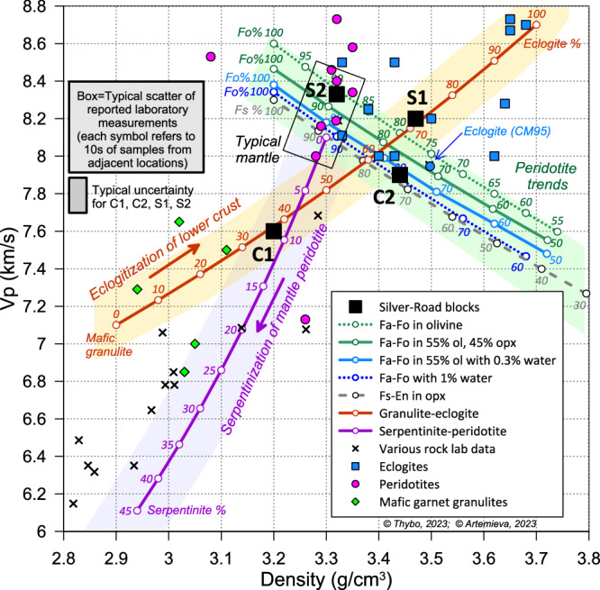
Lines show trends calculated based on laboratory data^39–42. Brown and purple curves illustrate the effects of metamorphic reactions from crustal mafic granulite to eclogite and from mantle peridotite to serpentinite (numbers show percentages of reaction products). A swarm of green and blue lines shows the effects of variation of iron (forsterite, Fo) and water content for various mantle peridotitic rocks. Black box shows typical upper mantle composition. Coloured bands illustrate uncertainties of calculated values. Symbols—averaged measured values for various crustal and mantle rocks; eclogite (CM95) is discussed in text. Black rectangular symbols show sub-Moho values in the central part of our profile (Fig. 5) in the 44–60 and 60–120 km depth intervals below the Scandes (C1, C2) and the Svecofennian shield (S1, S2), grey box shows the uncertainty. Fo forsterite, Fa fayalite, En enstatite, Fs ferrosilite, opx orthopyroxene, ol olivine.

We interpret the lithology below the seismic Moho along the profile by comparing our observed velocity and density values for the four characteristic units below the Caledonian and Svecofennian domains (C1, C2, S1, S2 in Fig. 5) with calculated values for peridotite, eclogite and serpentinite (Fig. 6) constrained by laboratory measurements^39–42.

Unit C1. The comparison of our density and P-wave velocity model with the experimental data suggests that C1 contains ~35% of eclogite at 44–60 km depth (Fig. 6). This eclogitic body below the Scandes may have formed when tectonics brought the lower crust to deep levels by the load of the probably more than ~8 km high Caledonian orogen⁸. Post-orogenic strong erosion and exhumation brought the eclogitic body to its present depth, and its upper boundary now forms the seismic Moho. C1 also plots close to the values for a 10% serpentinite formed from peridotite by a reaction, which requires water in the mantle. It is possible that serpentinite may have formed as a result of Caledonian subduction but we find this unlikely here because unit C1 extends for a very long distance of ~150 km (Fig. 5c) along a possible eastward dipping Caledonian subduction; furthermore, westward dipping Caledonian subduction structure under present-day Greenland⁴³ complicates the tectonic scenario.

Unit S1. The uppermost mantle in the Svecofennian shield at 44–60 km depth (S1) has too large density (3.47 g cm⁻³, Fig. 5) for a peridotite of any composition, and we interpret that it consists of mafic rocks that were eclogitized in the Proterozoic with possible Caledonian reworking to a metamorphic grade of 70% (S1 in Fig. 6), similar to the finding of a large eclogitic body further south in the Baltic Shield³⁶. The Proterozoic age of eclogitization is supported by Proterozoic subduction in region⁴⁴, which led to metal ore mineralisation in the Silver-Road region⁴⁵.

Unit S2. The deeper shield mantle at 60–120 km depth consists of a fertile peridotite with a bulk Mg# of ~90 (S2 in Fig. 6) in accordance with global geochemical data⁴⁶ and results of regional teleseismic travel time inversion¹⁵, but in contrast to the mantle composition of the Archean part of Fennoscandia, where such fertile layer occurs at 180–240 km depth⁴⁷.

Unit C2. Although the lower body of the model below the Scandes (C2) appears exotic, one may speculate if eclogites are also present in this body. The high-density (3.47 g cm⁻³, C2 in Fig. 5) body below the Scandes at 60–120 km depth could potentially be explained by ~60% eclogitization of mafic lower crustal material, but the parameters do not plot on the eclogitization curve, and the unit has an unrealistic low velocity of ca. 7.9 km s⁻¹ (5% less than the average velocity in this depth interval in Fennoscandia¹⁵). A compilation of measurements on 58 specimens of 18 rock samples characterised as mafic eclogites (sampling locations unknown) provide average values of 3.48 g cm⁻³ for density and 7.95 km s⁻¹ for Vp velocity (blue circle³³ CM95 close to C2 in Fig. 6), which is close to our observation of 3.44 g cm⁻³ and ~7.9 km s⁻¹ in unit C2. However, it is unusual to observe sub-Moho rocks with such high density and low velocity, and a 60 km thick eclogitic layer is unlikely, since it would be gravitationally unstable⁴⁸. The low velocity also cannot be attributed to high temperature because this would also lower the density, contrary to our model.

The velocity and density values for body C2 are instead better explained by a peridotitic mantle rock, which is exceptionally enriched in iron (a bulk Mg# of ~80) with a 0.3–1.0% water enrichment (blue lines in Fig. 6). Such exceptional iron enrichment is possible in a metallogenic ore province as here⁴⁵, and it cannot be identified by electrical measurements due to its super-Curie temperature (more than 600 °C at 50 km depth⁴⁹). Therefore, we explain the deep body below the Scandes (C2) by a strongly metasomatised, fertile peridotitic mantle which, however, may also contain some “dripping” eclogite material⁵⁰.

Origin of the anomalous mantle units

We explain the remarkable sub-Moho velocity transition from low (~7.6 km s⁻¹, C1) to high ( ~ 8.2 km s⁻¹, S1) velocity at depths between 44 and 60 km (Fig. 2b) below the Caledonian and Svecofennian units by different eclogite grade in former mafic lower crust, similar to observations in Tibet^51,52. A requirement for the formation of metamorphic eclogite is that the mineral assemblages must be brought to depths larger than 45 km (~1.2 GPa) at temperature less than ~500 °C⁵³ in the presence of fluids to facilitate the metamorphic reaction^54,55. Such conditions were satisfied in the upper mantle of Fennoscandia at various periods in relation to palaeosubduction⁴⁴, and a large preserved Proterozoic eclogitic body has recently been identified in the Svecofennian shield³⁶. Conditions were also favourable for metamorphism during the Caledonian orogeny (490–390 Ma) when the very high mountain chain was supported by thick crust²³. Our interpretation of sub-Moho eclogites further is supported by the constant Moho depth of ~44 km extending across both the Caledonides and the Svecofennian shield, and by observation of a sharp velocity increase from the lower part of the crust (Vp ~6.9 km s⁻¹) to the uppermost mantle (7.6–8.2 km s⁻¹), which indicates absence of mafic lower crust, although a very thin mafic layer (7.1–7.3 km s⁻¹) may be present in parts of the Svecofennian domain (Fig. 2b).

The amount of eclogite formed by metamorphism of a mafic lower crust depends on the source rock composition, amount of available fluid, temperature, deformation rate, and the time during which the rock has been subject to the high-pressure metamorphism^56–58. Significant changes in mineral assemblages and composition can be caused by small changes in fluid concentration rather than being controlled by temperature, pressure and rock composition alone⁵⁷. Lower-crustal compositional heterogeneity produced by the long-term evolution of Fennoscandia⁵⁹ should have essentially controlled metamorphism during the Proterozoic and Phanerozoic collisions. A comparison of our modelling results with regional and global field observations and laboratory measurements provides a frame for speculation on the origin of the anomalous upper mantle units below the Caledonian and Svecofennian units.

The low-density, sub-Moho body below the northern Scandes (C1, Fig. 5c) has density values of 3.20 g cm⁻³ as the reported average for anorthositic eclogites in the Bergen arc of Fennoscandia⁵⁸, with a P-wave velocity of 7.6 km s⁻¹ (Fig. 2b, Supplementary Fig. 11) in agreement with the estimated eclogite fraction of ~35% in the lower crustal material, which now is located below the seismic Moho. It suggests that the sub-Moho unit C1 in the northern Scandes contains anorthositic eclogites comparable to the Bergen arc eclogites with various degree of metamorphism from ~550 °C, 12 kbar inland to ~800 °C, 16–20 kbar at the coast⁶⁰.

The high-density 3.47 g cm⁻³, high-velocity (8.2 km s⁻¹) sub-Moho layer to 60 km depth in the Svecofennian domain (S1), interpreted by 70% eclogitization, has parameters similar to highly metamorphosed (80%) mafic eclogites mapped in southern Norway and China^37,57. The observed density and velocity values are comparable to the values for a similar sub-Moho eclogitic body observed in middle Fennoscandia and interpreted by Palaeoproterozoic 50–70% transformation of the mafic lowermost crustal layer into eclogite facies without later delamination³⁶. The metamorphic reaction was significantly influenced by fluids and deformation to result in such almost fully (70%) metamorphosed eclogites. The original Precambrian metamorphism may have been reactivated during the Caledonian orogeny when this part of the Fennoscandian lower crust again was depressed to large depth²³.

Seismic tomography indicates a highly heterogeneous upper mantle below Fennoscandia¹⁵ with dominant vertical layering in the Svecofennian shield⁶¹, similar to results from petrologic studies of mantle xenoliths in cratons^62,63, including the Baltic shield⁴⁷, and geophysical observations in cratons globally^64,65. Our findings are in agreement with these observations, and they indicate a significant role of eclogitization of lower crustal material in the evolution of the immediate sub-Moho mantle in cratons, cf. unit C1 in the Caledonian domain and S1 in the Svecofennian domain (Fig. 6). The deeper unit S2 in the Svecofennian domain (60–120 km depth) has velocity compatible with classic peridotitic mantle of Proterozoic age^34,46, which adds credibility to the interpretation of eclogitic material with various eclogite content in the lower crustal material in the sub-Moho depth interval down to 60 km in units C1 and S1.

Our velocity-density model explains the observed seismic velocity, gravity and topography around the northern Scandes by isostasy in the depth interval down to 120 km depth, which corresponds to the lower limit of a pronounced low-velocity anomaly observed by finite-frequency seismic tomography¹⁵. The unusual high-density, low-velocity layer below the Scandes (C2) is coincident with the extension of TIB below the Caledonian orogenic cover as exposed along the profile (Fig. 1b). The presence of TIB below the Caledonides indicates that this part of the mantle has been reworked during late Palaeoproterozoic magma emplacement. The lithosphere structure of this layer may further have been affected during the 350 My long extensional period⁶⁶ up to the break-up of the North Atlantic Ocean around 55 Ma. Later topographic change is primarily driven by enhanced erosion due to climate change and glaciations¹⁸.

Our model of the crustal and upper mantle density and velocity structure along the Silver-Road profile (Figs. 2b and 5c) demonstrates the presence of abrupt strong vertical and horizontal variation in the upper mantle composition, but not in the seismically defined crust. It indicates that large amounts of eclogite were formed by metamorphism in the mafic lower crust during various geologic periods with significantly different metamorphic imprint in the Scandes and the Svecofennian shield. Geophysically, the eclogitic bodies now appear as part of the uppermost mantle, where their tops define the seismic Moho and their bases define the petrological Moho. The sharp decrease in their metamorphic grade from the Svecofennian shield to the Caledonides provides isostatic support for the enigmatic Scandes mountain range, and suggests that collision, subduction, and magmatic activity may lead to asymmetric crustal densification and may play an important role in the topography formation of mountain ranges far from active plate boundaries. The observed >300 km long inland extent of the eclogitic material in different metamorphic grades (units C1, C2, S1) is remarkable and suggests that the amount of sub-Moho eclogite could be essentially underestimated globally.

Methods

Definition of some important geological terms

Moho – the seismic interface where the P-wave velocity increases to above ~7.6 km s⁻¹; it is mostly a strong seismic reflector. Reflections from the Moho are termed PmP and the velocity directly below the Moho is termed Pn velocity. Crust-mantle interface—the petrological transition from mafic to ultra-mafic rocks, which not always coincides with the Moho. Eclogites—here used to refer to eclogitic rocks formed from lower crustal, mafic rocks by high-pressure metamorphism. Fennoscandia—the geographic area consisting of Scandinavia and Finland; the Baltic Shield—the major, cratonic part of Fennoscandia which lacks a sedimentary cover and includes an Archaean nucleus in the north, to which a series of terranes and micro-continents amalgamated during the Svecofennian, Sveconorwegian and Caledonian orogenies; Svecofennian shield—the Svecofennian orogenic part of the Baltic Shield; Caledonides—the Caledonian deformed western part of Fennoscandia, possibly representing a series of nappes over original shield type crust; Scandes—the mountain range in western Fennoscandia along the North Atlantic coast which largely coincides with the Caledonides.

Seismic data

Our 380 km long refraction/wide-angle reflection profile, sub-perpendicular to the coastline, was acquired in July 2016 in northern Scandinavia between 67.6° N/13° E and 65.6° N/19.5° E. It extends from ca. 80 km offshore, across the Caledonides in the region of the high topography of the northern Scandes, and into the Svecofennian unit of Fennoscandia with moderate topography (Fig. 1a, b). Our seismic profile is based on data from 272 onshore stations, which recorded the seismic signal from five onshore explosive sources and twelve stacks of airgun shots (AGS) in the offshore part of the profile, sourced from vessel Hakon Mosby (Fig. 1a). The nominal station spacing is 1.1 km, the onshore source spacing is ~75 km, and airgun stacks are calculated at 3 km intervals. The 170 Texan and 102 Sercel instruments were equipped with 4.5 Hz vertical component geophones (Supplementary Table 1). Data were resampled to 6 ms before processing and modelling. The onshore seismic sources consist of two end-shots each charged with 400 kg chemical explosives (shots SP1 and SP5) and 200 kg charges at shot points SP2, SP3, and SP4 (Fig. 1a and Supplementary Table 2). All shots included multiple boreholes, each charged with ~50 kg of explosives above the base of the boreholes at a depth of ~50 m. Each airgun stack is calculated by stacking of 18 individual recordings of signals from a 22 liter large airgun array (Supplementary Table 2).

Seismic data analysis

The interpretation of the seismic data includes phase correlation and travel time picking of the refraction and reflection seismic phases (P_g, P₁, P_c1P, P₂, P_c2P, P_mP, P_n) from the crust and uppermost mantle (Fig. 2 and Supplementary Figs. 2–10), and subsequent forward modelling of the crustal velocity structure by raytracing travel time fitting. The Szplot software package⁶⁷, modified by P. Środa, was used for phase correlation and travel time picking, taking reciprocity into account. The seismic model was modelled with the rayinvr software⁶⁷ through the graphical user interface Pray⁶⁸, which allows interactive editing of the velocity model. The software uses a raytracing method for forward calculation of travel times and synthetic seismograms and for iterative inversion for optimum determination of selected model parameters. The 2-D velocity model is derived by applying a top-down scheme where the shallowest velocity layers are first determined, followed by subsequently deeper layers for the P-wave travel times.

Resolution of the seismic model

Overall, the model resolves the upper 50 km vertically. Vp velocities are constrained down to this depth at profile distance 0 to 250 km horizontally. The diagonal values of the resolution matrix are used to determine the depth and velocity resolution of the model⁶⁹. Parameters in the velocity model are considered well-constrained if the diagonal value of the resolution matrix exceeds 0.5 within a depth range of Δd = ±2 km or a velocity range of ΔV = ± 0.2 km s⁻¹. The area covered by seismic rays encompasses almost all parameter nodes, which all are constrained within the resolution criteria, i.e. they are resolved within ±2 km and ±0.2 km s⁻¹ (Supplementary Fig. 1a). However, the top of the lower crust is slightly less well resolved due to a limited number of travel time observations for P₂ and P_c2P (e.g. Supplementary Fig. 1, 5, 6, and 9). The offshore part of the model is constrained by the results of an earlier OBS profile²⁴.

Travel time fit of seismic phases

The seismic sections from onshore explosions (SP) and stacks of airgun shots (AGS) are of high quality. The correlated P-wave phases have clear onsets, which allow precise determination of their arrival times. The first arrival, refracted phases are observed across the whole onshore profile. The refracted phases from the crust (P_g, P₁, P₂) are correlated as first arrivals to around 200 km offset, where the sub-Moho P_n becomes first arrival out to 300 km offset. The refracted phase P₂ from the lower crust is also identified as a secondary arrival behind the P_n where it merges with the P_mP reflection. We identify two intra-crustal reflection phases P_c1P, P_c2P, and the P_mP reflection from the Moho. Reciprocity is checked for all interpreted phases. All phases can be reliably picked and the the refracted, first-arrival phases have high signal-to-noise ratio.

The P_g phase from the upper crust is observed out to 100–120 km offset in all sections. P₁ is observed on all sections to around 210 km offset with a higher apparent velocity than P_g, ranging between 6.3 and 6.5 km s⁻¹. The corresponding reflection phase P_c1P is observed at 80–120 km offset in all onshore shot sections. The refraction P₂ from the lower crust is observed in the offset interval 200–300 km in the long-range shot point sections (Sp1, Sp2 and SP5) with an apparent velocity of 6.7–6.8 km s⁻¹ with the matching P_c2P reflection only observed in the SP1 section in the western part of the model.

The P_mP phase is observed along the whole profile (Supplementary Figs. 10–12) with variable waveform and amplitude providing reflection coverage of the Moho from km 0 to km 250. The amplitude is weaker below the Scandes than in the Svecofennian part of the profile, where the model includes a strong velocity contrast across the Moho.

The P_n phase is observed as a clear first-arrival phase at offsets between 200 km and the end of each section in all sections with reversed coverage of the profile from 60 to 250 km (Supplementary Figs. 2–12). It provides good ray coverage of the uppermost mantle along the whole profile. The observed P_n phases all show direct connection to the critical P_mP reflection demonstrating that the picked PmP phase are reflections from the Moho.

The resulting 2-D raytracing velocity model (Fig. 2b) explains 99% of the picked travel times (Supplementary Table 3). The RMS travel time residual (t_RMS) is 76 ms, corresponding to 88 ms for onshore sources and 53 ms for the airgun shots (Supplementary Tables 2 and 3). We estimate the uncertainty of the picked travel times to be 75 ms for the refracted crustal phases (P_g, P₁ and P₂) and 100 ms for all other phases, which is a conservative estimate. The calculated χ² of the travel time residual is 0.9, corresponding to 1.3 for the onshore sources and 0.4 for the airgun stacks (Supplementary Tables 3–5).

Gravity test

We convert initially the P-wave velocity profile to a two-dimensional density section by using a standard velocity-density relation^31,32. This section is then used for 2-D modelling the density distribution along the seismic profile by iteratively fitting calculated gravity for the model with the observed Bouguer gravity anomalies from the EGM2008 gravity model⁷⁰ by using the GM-SYS (Geosoft Oasis Montaj) software. The initial density model basically fits all gravity data points. By slight modification of the initial density model (by less than 0.10 g cm⁻³ and generally less than 0.05 g cm⁻³), we obtain a fit to the gravity data better than 20 mGal.

Our first model extends to 60-km depth, where a recent regional S-wave receiver function study shows a strong positive converter in the area around our profile²⁹. The density model consists of four main layers including almost homogeneous top, middle, and lower crust with densities of 2.72, 2.84, and ~3.00 g cm⁻³. Similar to the velocity model, the main density variation is found in the upper mantle with densities of 3.24 g cm⁻³ below the thinned offshore crust, a similar low-density body (3.22 g cm⁻³) in the sub-Moho low-velocity region below the high topography of the Scandes, and an exceptionally high density of 3.47 g cm⁻³ in the Svecofennian unit (Fig. 4c). This model fits the observed Bouguer gravity anomaly within ±11 mGal (Fig. 4b). However, a calculated hypsometry profile, assuming vertical isostasy, shows very large elevation differences to the observed topography, i.e. the model predicts a ~2.9 km high mountain range, where the observed height is <1 km (Fig. 4a).

To fit the observed topography, we extend the model to 120 km depth, keeping its upper part similar to the first model. The 120 km compensation depth is chosen to incorporate the results of a recent teleseismic tomography study¹⁵ which includes a very low P-wave velocity anomaly (−5% with respect to the regional average) in the upper mantle down to a depth of ~120 km.

The free air gravity anomaly (FA) is close to zero along most of the profile and below the highest topography such that we may assume isostatic equilibrium. The FA variation between +10 and -25 mGal in the coastal zone (Fig. 5b) may be caused by lithosphere flexure. To account for possible deviation from isostatic equilibrium, we include the FA values into our calculation of predicted topography. Similar to isostatic calculations, where FA is assumed zero, the topography (t) above sea level is calculated from the equation

$$\mathrm{FA}=2\mathrm{\pi }\mathrm{G}\left(t{\rho }_1+{\Sigma h}_i{\rho }_i\right)$$ 1

where G is the gravity constant, ρ₁ is the density of the upper layer in the model, and the second term is the sum of the products of density ρ_i and thickness h_i of the layers between sea level and the compensation depth.

To fit both the observed Bouguer gravity anomaly and topography, the mantle interval between 60 and 120 km depth requires high densities of 3.47 g cm⁻³ in unit C2 below the high-topography Scandes, located between zones with “normal” peridotitic upper mantle densities (~ 3.36 g cm⁻³) both towards the ocean and in the Svecofennian shield (Fig. 5c). In comparison to our first gravity model, only minor changes are required for the crustal and mantle densities in the upper 60 km. The adjustment of densities includes changes from 2.94 to 2.87 g cm⁻³ and from 3.03 to 3.00 g cm⁻³ for the lower crustal part in the Caledonian and Svecofennian parts, respectively, as well as from 3.22 to 3.20 g cm⁻³ for the shallow sub-Moho layer below the Scandes (C1), while keeping unchanged the sub-Moho density below the Svecofennian unit (S1). With these slight changes, the model explains both the observed Bouguer anomaly and the hypsometry (Fig. 5).

Extensive sensitivity tests of the key parameters for units C1, C2, S1, and S2 (Supplementary Figs. 13–16) show that the final density model shows a perfect match of topography within 130 m (Fig. 5a) and the Bouguer anomaly within 24 mGal (Fig. 5b). The densities of units C1 and S1 between ~45 and 60 km depth are well-constrained within 0.04 g cm⁻³, and the densities of the large units C2 and S2 between 60 and 120 km depth are constrained within 0.02 g cm⁻³. Teleseismic tomography has a relatively low vertical resolution, so we test the importance of the chosen exact depth to the base of the density model by sensitivity analysis, by which we find that the exact choice is insignificant for the determined densities (Supplementary Figs. 17 and 18).

Author contributions

H.T. initiated and designed the research. A.S. was the chief scientist on board MS Hakon Mosby. H.T., I.M.A., P.H., and R.M. participated in the onshore field work. M.K. modelled the seismic and gravity data under detailed instruction and supervision by H.T. The interpretation was developed by H.T. and I.M.A. The initial manuscript draft was written by H.T. and all authors read and accepted the manuscript. M.K., I.M.A., and H.T. drafted the illustrations.

Peer review

Peer review information

Nature Communications thanks Irene DeFelipe, Ramon Carbonell, and the other, anonymous, reviewer(s) for their contribution to the peer review of this work. A peer review file is available.

Data availability

All data are available in the manuscript, including Supplementary Figs. 2–10, as well as by request to H. Thybo at h.thybo@gmail.com.

Code availability

The Szplot and rayinvr computer codes are available from the author, Dr. Colin Zelt at his website: https://terra.rice.edu/department/faculty/zelt/, and the Pray code is available from ref. ⁶⁸. The GM-SYS software is available from the developer: https://www.seequent.com/products-solutions/geosoft-oasis-montaj/gm-sys/.

Competing interests

The authors declare no competing interests.

Supplementary information

The online version contains supplementary material available at 10.1038/s41467-025-55865-3.

References

- 1.Japsen, P., Chalmers, J. A., Green, P. F. & Bonow, J. M. Elevated, passive continental margins: not rift shoulders, but expressions of episodic, post-rift burial and exhumation. Glob. Planet Change90–91, 73–86 (2012). [Google Scholar]
- 2.Lithgow-Bertelloni, C. & Silver, P. G. Dynamic topography, plate driving forces and the African superswell. Nature395, 269–272 (1998). [Google Scholar]
- 3.Walker, R. T. et al. Rapid mantle-driven uplift along the Angolan margin in the late Quaternary. Nat. Geosci.9, 909–914 (2016). [Google Scholar]
- 4.Faleide, J. I. et al. Structure and evolution of the continental margin off Norway and the Barents Sea. Episodes31, 82–91 (2008). [Google Scholar]
- 5.Anell, I., Thybo, H. & Artemieva, I. M. Cenozoic uplift and subsidence in the North Atlantic region: geological evidence revisited. Tectonophysics474, 78–105 (2009). [Google Scholar]
- 6.Nielsen, S. B. et al. The ICE hypothesis stands: how the dogma of late Cenozoic tectonic uplift can no longer be sustained in the light of data and physical laws. J. Geodyn.50, 102–111 (2010). [Google Scholar]
- 7.Japsen, P., Bonow, J. M., Green, P. F., Chalmers, J. A. & Lidmar-Bergström, K. Elevated, passive continental margins: Long-term highs or Neogene uplifts? New evidence from West Greenland. Earth Planet Sci. Lett.248, 330–339 (2006). [Google Scholar]
- 8.Gabrielsen, R. H. et al. Latest Caledonian to Present tectonomorphological development of southern Norway. Mar. Pet. Geol.27, 709–723 (2010). [Google Scholar]
- 9.Molnar, P. & England, P. Late Cenozoic uplift of mountain ranges and global climate change: chicken or egg? Nature346, 29–34 (1990). [Google Scholar]
- 10.Ebbing, J. & Olesen, O. The Northern and Southern Scandes—structural differences revealed by an analysis of gravity anomalies, the geoid and regional isostasy. Tectonophysics411, 73–87 (2005). [Google Scholar]
- 11.Stratford, W. & Thybo, H. Seismic structure and composition of the crust beneath the southern Scandes, Norway. Tectonophysics502, 364–382 (2011). [Google Scholar]
- 12.Kvarven, T. et al. Crustal composition of the Møre Margin and compilation of a conjugate Atlantic margin transect. Tectonophysics666, 144–157 (2016). [Google Scholar]
- 13.Frassetto, A. & Thybo, H. Receiver function analysis of the crust and upper mantle in Fennoscandia—isostatic implications. Earth Planet Sci. Lett.381, 234–246 (2013). [Google Scholar]
- 14.Mansour, W. Ben, England, R. W., Fishwick, S. & Moorkamp, M. Crustal properties of the northern Scandinavian mountains and Fennoscandian shield from analysis of teleseismic receiver functions. Geophys J. Int.214, 386–401 (2018). [Google Scholar]
- 15.Bulut, N., Thybo, H. & Maupin, V. Highly heterogeneous upper-mantle structure in Fennoscandia from finite-frequency P-body-wave tomography. Geophys J. Int.230, 1197–1214 (2022). [Google Scholar]
- 16.Milne, G. A. et al. Space-geodetic constraints on glacial isostatic adjustment in Fennoscandia. Science291, 2381–2385 (2001). [DOI] [PubMed] [Google Scholar]
- 17.Simons, M. & Hager, B. H. Localization of the gravity field and the signature of glacial rebound. Nature390, 500–504 (1997). [Google Scholar]
- 18.Anell, I., Thybo, H. & Stratford, W. Relating Cenozoic North Sea sediments to topography in southern Norway: the interplay between tectonics and climate. Earth Planet Sci. Lett.300, 19–32 (2010). [Google Scholar]
- 19.Rohrman, M., van der Beek, P. A., van der Hilst, R. B. R. D. & Reemst, P. Timing and mechanisms of North Atlantic Cenozoic uplift: evidence for mantle upwelling. Geol. Soc. Spec. Publ.196, 27–43 (2002). [Google Scholar]
- 20.Schoonman, C. M., White, N. J. & Pritchard, D. Radial viscous fingering of hot asthenosphere within the Icelandic plume beneath the North Atlantic Ocean. Earth Planet Sci. Lett.468, 51–61 (2017). [Google Scholar]
- 21.Makushkina, A., Tauzin, B., Tkalčić, H. & Thybo, H. The mantle transition zone in Fennoscandia: enigmatic high topography without deep mantle thermal anomaly. Geophys Res. Lett.46, 3652–3662 (2019). [Google Scholar]
- 22.Gaal, G. & Gorbatschev, R. An outline of the Precambrian evolution of the Baltic Shield. Precambrian Res35, 15–52 (1987). [Google Scholar]
- 23.Gee, D. G., Fossen, H., Henriksen, N. & Higgins, A. K. From the early Paleozoic platforms of Baltica and Laurentia to the Caledonide Orogen of Scandinavia and Greenland. Episodes31, 44–51 (2008). [Google Scholar]
- 24.Mjelde, R., Sellevoll, M. A., Shimamura, H., Iwasaki, T. & Kanazawa, T. Crustal structure beneath Lofoten, N. Norway, from vertical incidence and wide‐angle seismic data. Geophys J. Int114, 116–126 (1993). [Google Scholar]
- 25.Schmidt, J. Deep Seismic Studies in the Western Part of the Baltic Shield. 147 pp. (PhD thesis, Uppsala University, 2000).
- 26.Lund, C. E. The fine structure of the lower lithosphere underneath the Blue Road profile in northern Scandinavia. Tectonophysics56, 111–122 (1979). [Google Scholar]
- 27.Maupin, V. et al. The deep structure of the Scandes and its relation to tectonic history and present-day topography. Tectonophysics602, 15–37 (2013). [Google Scholar]
- 28.Artemieva, I. M. & Thybo, H. EUNAseis: a seismic model for Moho and crustal structure in Europe, Greenland, and the North Atlantic region. Tectonophysics609, 97–153 (2013). [Google Scholar]
- 29.Makushkina, A., Tauzin, B., Miller, M. S., Tkalcic, H. & Thybo, H. Opening of the North Atlantic Ocean and the rise of Scandinavian mountains. Geology10.1130/G52735.1 (2025).
- 30.Thybo, H. et al. Scanarray—a broadband seismological experiment in the Baltic Shield. Seismol Res. Lett.92, 2811–2823 (2021). [Google Scholar]
- 31.Herceg, M., Artemieva, I. M. & Thybo, H. Sensitivity analysis of crustal correction for calculation of lithospheric mantle density from gravity data. Geophys. J. Int.204, 687–696 (2016). [Google Scholar]
- 32.Brocher, T. M. Empirical relations between elastic wavespeeds and density in the Earth’s crust. Bull. Seis Soc. Am.95, 2081–2092 (2005). [Google Scholar]
- 33.Christensen, N. I. & Mooney, W. D. Seismic velocity structure and composition of the continental crust: a global view. J. Geophys Res.100, 9761–9788 (1995). [Google Scholar]
- 34.James, D. E., Boyd, F. R., Schutt, D., Bell, D. R. & Carlson, R. W. Xenolith constraints on seismic velocities in the upper mantle beneath southern Africa. Geochem. Geophys. Geosyst.10.1029/2003GC000551 (2004).
- 35.Rudnick, R. L. & Fountain, D. M. Nature crust: and composition of the continental perspective. Rev. Geophys.3, 267–309 (1995). [Google Scholar]
- 36.Buntin, S. et al. Long-lived Paleoproterozoic eclogitic lower crust. Nat. Commun.10.1038/s41467-021-26878-5 (2021). [DOI] [PMC free article] [PubMed]
- 37.Wang, Q., Burlini, L., Mainprice, D. & Xu, Z. Geochemistry, petrofabrics and seismic properties of eclogites from the Chinese Continental Scientific Drilling boreholes in the Sulu UHP terrane, eastern China. Tectonophysics475, 251–266 (2009). [Google Scholar]
- 38.Mjelde, R., Kvarven, T., Faleide, J. I. & Thybo, H. Lower crustal high-velocity bodies along North Atlantic passive margins, and their link to Caledonian suture zone eclogites and Early Cenozoic magmatism. Tectonophysics670, 16–29 (2016). [Google Scholar]
- 39.Mizutani, H., Hamano, Y., Ida, Y. & Akimoto, S. Compressional-wave velocities of fayalite, Fe 2 SiO 4 spinel, and coesite. J. Geophys. Res.75, 2741–2747 (1970). [Google Scholar]
- 40.Sinogeikin, S. & Bass, J. Single-crystal elastic properties of chondrodite: implications for water in the upper mantle. Phys. Chem. Miner.26, 297–303 (1999). [Google Scholar]
- 41.Christensen, N. I. Serpentinites, peridotites, and seismology. Int. Geol. Rev.46, 795–816 (2004). [Google Scholar]
- 42.Artemieva, I. The Lithosphere: An Interdisciplinary Approach (Cambridge University Press, 2011).
- 43.Schiffer, C., Balling, N., Jacobsen, B. H., Stephenson, R. A. & Nielsen, S. B. Seismological evidence for a fossil subduction zone in the East Greenland Caledonides. Geology42, 311–314 (2014). [Google Scholar]
- 44.BABEL Working Group. Evidence for early Proterozoic plate tectonics from seismic reflection profiles in the Baltic Shield. Nature348, 34–38 (1990). [Google Scholar]
- 45.Frietsch, R., Papunen, H. & Vokes, F. M. The ore deposits in Finland, Norway, and Sweden; a review. Econ. Geol.74, 975–1001 (1979). [Google Scholar]
- 46.Gaul, O. F., Griffin, W. L., O’Reilly, S. Y. & Pearson, N. J. Mapping olivine composition in the lithospheric mantle. Earth Planet Sci. Lett.182, 223–235 (2000). [Google Scholar]
- 47.Lehtonen, M. L., O’Brien, H. E., Peltonen, P., Johanson, B. S. & Pakkanen, L. K. Layered mantle at the Karelian Craton margin: P-T of mantle xenocrysts and xenoliths from the Kaavi-Kuopio kimberlites, Finland. Lithos77, 593–608 (2004). [Google Scholar]
- 48.Houseman, G. A. & Molnar, P. Gravitational (Rayleigh-Taylor) instability of a layer with non-linear viscosity and convective thinning of continental lithosphere. Geophys J. Int.128, 125–150 (1997). [Google Scholar]
- 49.Artemieva, I. M. Global 1° × 1° thermal model TC1 for the continental lithosphere: Implications for lithosphere secular evolution. Tectonophysics416, 245–277 (2006). [Google Scholar]
- 50.Göǧüş, O. H., Pysklywec, R. N., Şengör, A. M. C. & Gün, E. Drip tectonics and the enigmatic uplift of the Central Anatolian Plateau. Nat. Commun.10.1038/s41467-017-01611-3 (2017). [DOI] [PMC free article] [PubMed]
- 51.Nábelek, J. et al. Underplating in the Himalaya-Tibet collision zone revealed by the Hi-CLIMB experiment. Science325, 1371–1371 (2009). [DOI] [PubMed] [Google Scholar]
- 52.Wang, G., Thybo, H. & Artemieva, I. M. No mafic layer in 80 km thick Tibetan crust. Nat. Commun.12, 4–12 (2021). [DOI] [PMC free article] [PubMed] [Google Scholar]
- 53.Liou, J. G., Hacker, B. R. & Zhang, R. Y. Into the Forbidden zone. Science287, 1215–1216 (2000). [Google Scholar]
- 54.Philippot, P. Fluid-melt rock interaction in mafic eclogites and coesite-bearing metasediments—constraints on volatile recycling during subduction. Chem. Geol.108, 1–4 (1993). [Google Scholar]
- 55.Lee, C.-T. A. Trace element evidence for hydrous metasomatism at the base of the North American lithosphere and possible association with Laramide low-angle subduction. J. Geol.113, 673–685 (2005). [Google Scholar]
- 56.Ahrens, T. J. & Schubert, G. Rapid formation of eclogite in a slightly wet mantle. Earth Planet Sci. Lett.27, 90–94 (1975). [Google Scholar]
- 57.Austrheim, H. Eclogitization of lower crustal granulites by fluid migration through shear zones. Earth Planet Sci. Lett.81, 221–232 (1987). [Google Scholar]
- 58.Austrheim, H. The granulite-eclogite facies transition: a comparison of experimental work and a natural occurrence in the Bergen Arcs, western Norway. Lithos25, 163–169 (1990). [Google Scholar]
- 59.Peltonen, P., Mänttäri, I., Huhma, H. & Whitehouse, M. J. Multi-stage origin of the lower crust of the Karelian craton from 3.5 to 1.7 Ga based on isotopic ages of kimberlite-derived mafic granulite xenoliths. Precambrian Res.147, 107–123 (2006). [Google Scholar]
- 60.Austrheim, H. & Griffin, W. L. Shear deformation and eclogite formation within granulite-facies anorthosites of the Bergen Arcs, western Norway. Chem. Geol.50, 267–281 (1985). [Google Scholar]
- 61.Thybo, H. & Perchuć, E. The seismic 8° discontinuity and partial melting in continental mantle. Science10.1126/science.275.5306.162 (1997). [DOI] [PubMed]
- 62.Griffin, W. L. et al. The Kharamai kimberlite field, Siberia: modification of the lithospheric mantle by the Siberian Trap event. Lithos81, 167–187 (2005). [Google Scholar]
- 63.Kopylova, M. G. & Russell, J. K. Chemical stratification of cratonic lithosphere: constraints from the Northern Slave craton, Canada. Earth Planet Sci. Lett. 10.1016/S0012-821X(00)00187-4 (2000).
- 64.Yuan, H. & Romanowicz, B. Lithospheric layering in the North American craton. Nature466, 1063–1068 (2010). [DOI] [PubMed] [Google Scholar]
- 65.Yang, H., Artemieva, I. M. & Thybo, H. The mid-lithospheric discontinuity caused by channel flow in proto-cratonic mantle. J. Geophys. Res. Solid Earth128, e2022JB026202 (2023).
- 66.Ziegler, P. A. & Cloetingh, S. Dynamic processes controlling evolution of rifted basins. Earth Sci. Rev.64, 1–50 (2004). [Google Scholar]
- 67.Zelt, C. A. & Smith, R. B. Seismic traveltime inversion for 2‐D crustal velocity structure. Geophys J. Int.108, 16–34 (1992). [Google Scholar]
- 68.Fromm, T. PRay—a graphical user interface for interactive visualization and modification of rayinvr models. J. Appl. Geophys.124, 1–3 (2016). [Google Scholar]
- 69.Zelt, C. A. Modelling strategies and model assessment for wide-angle seismic traveltime data. Geophys J. Int.139, 183–204 (1999). [Google Scholar]
- 70.Pavlis, N. K., Holmes, S. A., Kenyon, S. C. & Factor, J. K. The development and evaluation of the Earth Gravitational Model 2008 (EGM2008). J. Geophys. Res. Solid Earth117, 1–38 (2012). [Google Scholar]
Associated Data
This section collects any data citations, data availability statements, or supplementary materials included in this article.
Supplementary Materials
Data Availability Statement