

Abstract
Inferring appropriate synthesis reaction (i.e., retrosynthesis) routes for newly designed molecules is vital. Recently, computational methods have produced promising single-step retrosynthesis predictions. However, template-based methods are limited by the known synthesis templates; template-free methods are weakly interpretable; and semi template-based methods are deficient with regard to utilizing the associations between chemical entities. To address these issues, this paper leverages the intra-associations between synthons, the inter-associations between synthons and leaving groups (LGs), and the intra-associations between LGs. It develops a multitask graph representation learning model for single-step retrosynthesis prediction (Retro-MTGR) to solve reaction centre deduction and LG identification simultaneously. A comparison with 16 state-of-the-art methods first demonstrates the superiority of Retro-MTGR. Then, its robustness and scalability and the contributions of its crucial components are validated. More importantly, it can determine whether a bond can be a reaction centre and what LGs are appropriate for a given synthon, respectively. The answers reflect underlying chemical synthesis rules, especially opposite electrical properties between chemical entities (e.g., reaction sites, synthons, and LGs). Finally, case studies demonstrate that the retrosynthesis routes inferred by Retro-MTGR are promising for single-step synthesis reactions. The code and data of this study are freely available at 10.5281/zenodo.14346324.
Subject terms: Computational chemistry, Cheminformatics
Machine learning can be used to infer proper retrosynthesis routes for newly designed molecules. Here, the authors develop a multitask graph representation learning model for single-step retrosynthesis inference by exploiting chemical synthesis rules among different entity.
Introduction
In diverse modern drug design tasks (e.g., target screening1, molecule generation2, and ADMET prediction3), artificial intelligence (AI) technologies have achieved promising progress with significant cost and time reductions4,5. Once the chemical structure of a small molecule is determined in silico, retrosynthesis inference can determine the available reactants for synthesizing the target molecule6. This retrosynthesis process works as a bridge from in silico to in vitro settings. Compared to the synthesis reaction, retrosynthesis is an inverse inference process7,8. A complete retrosynthesis process is a tree-like route9, where the root node (the target molecule) is recursively decomposed into its descendant nodes (reactants) until reaching reactants that are commercially available. Each decomposition stage is called a single-step retrosynthesis process. However, even inferring a single-step retrosynthesis relies heavily on the individual domain experiences of chemists under costly trial-and-error assays10.
In recent years, both the accumulation of chemical synthesis data and the growth of deep learning methods have accelerated the rapid development of computer-assisted synthesis processes (CASPs) for single-step retrosynthesis. The existing single-step retrosynthesis methods can be roughly grouped into template-based, template-free, and semi template-based methods11. Template-based methods infer the single-step retrosynthesis process of a newly given molecule by finding appropriate reaction templates. These techniques can be categorized into similarity-based, classification-based, and embedding-based approaches. Similarity-based approaches directly leverage similarity metrics to match the target molecule to pre-collected reaction templates. For example, Coley et al. utilized the Tanimoto similarity on Morgan molecular fingerprints to search for suitable retrosynthesis templates12. Dai et al. proposed a conditional graphical model constructed upon graph learning networks (GLNs) and performed subgraph pattern matching to acquire candidate templates13. Classification-based approaches, which treat templates as class labels and target molecules as samples, train multiclass classifiers to determine candidate templates for a given target molecule. For example, Segler et al. trained a multiclass deep neural network with extended-connectivity fingerprints (ECFP4) to infer appropriate templates14. After organizing templates into reaction type-specific groups, Baylon et al. trained a set of reaction type-specific deep highway networks with Morgan fingerprints to match the correct templates in each template group15. Embedding-based approaches map both target molecules and templates into a common embedding space, where a good match is declared if a template is near a target molecule. For instance, Chen et al. designed an MPNN variant (LocalRetro) to encode templates and target molecules16. Seidl et al. proposed a modern Hopfield network (MHN) to measure the relevance between templates and the target molecule (initialized by ECFPs)17. However, template-based methods cannot predict the retrosynthesis results of target molecules with novel synthesis patterns that are outside the synthesis rules contained in the utilized template library. In addition, it is tedious to update template libraries when new synthesis knowledge is discovered18. In contrast, both template-free and semi template-based methods can predict single-step retrosynthesis results without a prebuilt template library.
Inspired by machine translation, template-free methods directly convert the input target molecule into its reactants in the form of strings. The simplified molecular input line entry system (SMILES) is a string notation strategy for representing molecules and reactions. It is a true chemical notation language with a simple vocabulary, including atom symbols, bond symbols, branches, cyclic structures, disconnected structures, and no space19. Each unit in the SMILES can be regarded as a word in a machine translation model. This paradigm has boosted the development of template-free methods. In earlier years, Liu et al. proposed an attention-enhanced long short-term memory (LSTM) model20 to convert the target molecule into its reactants under a sequence-to-sequence encoder-decoder architecture21. As new superstars in the natural language processing domain, transformers22 have been directly applied to retrosynthesis prediction in recent years since a SMILES string is equivalent to a chemical notation sentence23,24. However, these methods have led to new issues in which the generated reactants are probably invalid in terms of chemistry. More efforts have been made to address this issue. Zheng et al. designed an extra syntax postchecker based on a transformer to satisfy the chemical validity requirements of generated reactants25. Ucak et al. treated molecular substructures (capturing their local atomic environments) as words in a transformer to guarantee the validity of the generated reactants26. Similarly, Fang et al. defined a vocabulary of atom-localized substructures to convert a SMILES string into a word sequence under the transformer architecture27. However, these methods using SMILES representations cannot effectively capture the rich information hidden in molecular chemical structures (e.g., atomic properties, bond features, and adjacent structure matrices28). The subsequently developed methods integrate structural information into transformer-based retrosynthesis prediction frameworks. Mao et al. proposed a graph attention network (GAT) to encode atoms on molecular graphs, enhancing the atom embeddings in transformers29. Wan et al. integrated the adjacent matrix of a molecular graph into the calculating self-attention values. Lin et al. enhanced a self-attention module via node centrality and node position encodings derived from bipartite molecular graphs30. Tu et al. utilized a directed message passing neural network (D-MPNN) on a molecular graph to encode atoms and directly used the decoder of a transformer to generate reactants31. However, since the process of generating SMILES strings in template-free approaches sequentially outputs individual symbols, the interpretability of the resulting predictions is limited32.
Inspired by the retrosynthesis inference process employed by chemists, semi template-based methods perform two-phase retrosynthesis prediction tasks, including reaction centre prediction and leaving group (LG) prediction. The former subtask finds the reaction centre (i.e., a bond consisting of two reaction sites) where the molecule of interest is split into two synthons (i.e., incomplete reactants)33. The latter infers appropriate functional groups (i.e., LGs) that attach to two synthons to form reactants. Analogous to template-free methods, some semi template-based methods still adopt translation models to perform two-phase retrosynthesis prediction. For example, Wang et al. formulated the reaction centre prediction and LG prediction tasks as two sequence-to-sequence problems (i.e., target molecules to synthons and synthons to reactants, respectively), which were solved by two independent transformers respectively34. To characterize the rich information possessed by molecular structures, some methods treat bonds as samples and utilize graph neural networks to achieve an improved reaction centre identification effect via bond classification. For instance, Shi et al. utilized relational graph convolutional networks (R-GCNs) to recognize reaction centres and converted completed synthons into reactants via a variational graph translation model35. Yan et al. applied a GAT variant to predict reaction centres and a sequence-based transformer to convert synthons into reactants36. To obtain improved reaction centre predictions with richer chemical meanings, graph editing operations (e.g., node/edge additions and deletions) were leveraged in the follow-up methods. Somnath et al. constructed MPNNs to encode atoms/bonds into embedding spaces, where predefined graph editing operations implemented on atoms/bonds were discriminated to determine the reaction centre, and candidate LGs autoregressively picked from a discrete LG vocabulary were subsequently utilized for determining the corresponding synthons37. Similarly, Chen et al. designed a graph message passing network (GMPN) to predict graph editing operations on product molecular graphs to obtain synthons38. Furthermore, they found appropriate LGs from a predefined LG list in an autoregressive manner38. Moreover, considering the connection between reaction centre prediction and LG prediction, some methods have integrated these tasks into a unified autoregressive reasoning process under graph editing operations. For example, by adopting the encoder-decoder architecture in a transformer22, Sacha et al. iteratively started multiple graph editing operations from the target molecule until a STOP operation was encountered (i.e., until its reactants were reached)39. Zhong et al. adopted a similar architecture but employed more detailed graph editing operations32. However, the existing methods are deficient in terms of utilizing the occurrence tendencies of LGs w.r.t. synthons and their co-occurring associations.
We consider three underlying associations between chemical entities in a chemical synthesis reaction, such as a broad-sense coupling reaction ‘’. Broad-sense coupling reactions are dominant in multi-step retrosynthesis40. The above case generates one product molecule from two reactant molecules, except for H2O. The first association accounts for the two synthons (i.e., and ) forming the product (i.e., ). The second is the association between the two LGs (i.e., and ) that form the side product (i.e., ). The third is the association between a synthon and its LG, which are dissociated from the corresponding reactant, such as the pair of and forming . Moreover, as stated by Ayers41, an excellent LG tends to be structurally simple (even monatomic) and to exhibit strong electron affinity and low bond dissociation energies (e.g., H, Cl, Br, and OH). We believe that structurally simple LGs are dominant w.r.t. the occurrence frequencies observed across molecules. In addition, we believe that bonds with strong energies tend to be ordinary bonds rather than reaction centres since it is difficult to synthesize high-energy bonds. Appropriately utilizing these associations would improve the interpretability of retrosynthesis prediction.
Following the abovementioned consideration in reactions, this work, treating products, reactants, and synthons as molecule graphs to obtain atom embeddings, aims to measure the associations among synthons and LGs in a chemical embedding space. To achieve this goal, it develops a Multi-Task Graph Representation learning framework for Retrosynthesis prediction (Retro-MTGR), which performs two tasks (i.e., reaction centre recognition and leaving group identification) in retrosynthesis (shown in Fig. 1). Its fundamental ideas are listed in the following:
Fig. 1. The framework of Retro-MTGR.

Molecules in the form of graphs are first represented by an MPNN-based atom encoder to learn initial atom embeddings. The AEE further boosts the atom embeddings by performing contrastive learning on the molecules and their synthons w.r.t. the associated molecule embeddings. The RCP implements a bond-level readout on the enhanced atom embeddings to learn bond embeddings, which are sequentially augmented by extra bond energies, and then recognize the reaction centres among the bonds. Afterwards, the LGP learns LG embeddings based on an LG co-occurrence graph and measures the proximity between them and the synthon embeddings (involving the atoms and bonds in the reaction centres) to predict appropriate LGs for the given synthons.
To make reaction sites (i.e., atoms in reaction centres) significant, Retro-MTGR elaborates an atom embedding enhancer (AEE), which captures the structural commonness and the differences between a product and the combination of its two synthons by graph-contrastive learning (GCL)42.
To highlight the difference between ordinary bonds and reaction centres, it constructs a reaction centre predictor (RCP), which generates bond embeddings augmented by easily accessed chemical knowledge (i.e., theoretical bond energies43).
To reveal the intra-associations/inter-associations between chemical entities (synthons and LGs) in reactions, the framework designs a leaving group predictor (LGP), which characterizes synthons by the embeddings of reaction sites (atoms) and reaction centres (bonds), represents LGs through embedding an LG co-occurrence network, and constructs a joint embedding space of synthons and LGs to measure their proximity.
The main findings of this work are stated as follows
Based on the clustering over the learned bond embeddings, the bond embedding space illustrates why a bond can be the reaction centre in synthesis reactions (based on both USPTO-50K and USPTO-480K). The observations include (1) double bonds (C = C, C = O, and C = N), triple bonds (C#C and C#N), and aromatic bonds (c ~ c and c ~ n) having high energy (>=360 kJ/mol) are ordinary bonds and belong to unique communities; (2) single bonds (i.e., C-C, C-c, c-c C’-C’, C’-O’, c-O, C’-N’, C-S, C-N and C-O) having low bond energies (<360 kJ/mol) fall into one community accounting for reaction centres and others accounting for ordinary bonds due to the diverse molecular structure topologies of their corresponding synthons44; (3) the electrical property distributions of the atom pairs contained in bonds demonstrate that a bond is the coupling reaction centre in a molecule if its member atoms tend to have opposite electrical properties (reflected by local substructures)45; otherwise, it is an ordinary bond.
The joint embedding space of chemical entities in reaction illustrates the distributions and the intra-associations/inter-associations of synthons and LGs. Four findings are concluded: (1) two synthons in a reaction always have opposite Eps (electrical properties) and are distant from each other; (2) a synthon and an LG belonging to a reactant usually have opposite EPs and are close to each other; (3) two LGs co-occurring in a reaction regularly have opposite EPs and are distant from each other; (4) in addition, reaction-common LGs tend to be spread around and are occurrence-dominant, monatomic or structurally simple (e.g., H, CL, Br, I, and OH), while reaction-specific LGs tend to gather w.r.t. their reaction types and are similar to each other in terms of structures.
Results
Dataset
As commonly done in the existing methods26, we collect our benchmark dataset from the USPTO-50K dataset, which was derived from an open-source patent database containing 50,016 atom-mapped reactions46. The USPTO-50K dataset contains 10 types of reactions, including six kinds of broad-sense coupling reactions and four types of other reactions. By forming the molecule scaffold, broad-sense coupling reactions are the majority in the multi-step synthesis of a product molecule47. For example, as we counted, they account for >80% of 1771 reactions in the multi-step retrosynthetic routes provided in the study of Kevin40. In contrast, deprotections, protections, reductions, and oxidations modify atoms in branches or small functional groups to increase yield rate and raw material availability48–50. Thus, in the field of retrosynthesis inference, our Retro-MTGR pays attention to the retrosynthesis of broad-sense coupling reactions, which are involved in the disconnection of the molecular scaffold. After discarding deprotection, protection, reduction, and oxidation reactions, our dataset contains 35,682 reaction entries of broad-sense coupling reactions, which are further divided into 6 categories according to their reaction types (Supplementary Table 1). Furthermore, we adopt the same training-validation-testing (TVTS) split as that used in the research of Coley et al.12; the reactions are decomposed into a training set, a validation set, and a testing set at an 8:1:1 ratio.
Parameter settings
In the atom encoder, as suggested by the existing methods3, each atom is initially represented by a 28-dimensional (28-d) atom feature vector , including the atom type (23-d), the number of hydrogens (1-d), the number of linking neighbours (degree, 1-d), whether the atom is aromatic (1-d), its formal charge (1-d), and its atomic mass (1-d). See Supplementary Table 2 for details.
Due to the one-hot f atom type coding process, the initial atom representation is semisparse. To learn better embeddings, as suggested by Cheng et al.51, an extra three-layer MLP maps the atom to a dense form (). We empirically set 64 and 32 neurons in the hidden and output layers, respectively.
Moreover, bonds are represented as a binary adjacent matrix , in which indicates the occurrence of a bond between two atoms ( and ); otherwise, no bond occurs. Both and are input into a multilayer MPNN to obtain atom embeddings with the same dimensions as those of . In particular, we investigate how the number of MPNN layers (#layers = 1, 2, 4, 6) influences the performance of Retro-MTGR under the selected TVTS split. As shown in Supplementary Fig. 1, the investigation (measured by top-1, top-3, and top-5 accuracy) reveals that the case with two layers yields the best performance in both the reaction-type-unknown (RTU) and reaction-type-known (RTK) scenarios.
In the RCP module, the MLP accounting for reaction centre identification also contains an input layer, a hidden layer, and an output layer. The input layer includes 33 neurons, where 32 neurons are responsible for the resulting embeddings derived from the bond-level readout, and the last neuron is responsible for the bond energy. The number of neurons is empirically set to 16. The unique neuron in the output layer accounts for the confidence score of a potential reaction centre.
In the LGP module, the nodes in the LGCoG are initially represented as -dimensional one-hot coding vectors , where is the cardinality of the LG set. Then, they are mapped to LG embeddings by another two-layer MPNN without undergoing dimensional changes. Additionally, the adaptor maps the synthon embedding space (the concatenation of 32-d atom embeddings and 33-d bond embeddings) to the LG embedding space. This mechanism is implemented by a three-layer MLP, which contains an input layer accounting for synthon embeddings (), a hidden layer empirically possessing 128 neurons, and an output layer with neurons. Thus, = , where (i.e., ) is scenario-specific since the type-known scenario and the type-unknown scenario have different types of LGs.
Finally, to investigate how the task weights influence the prediction results, we perform multiple rounds of parameter tuning in the RTU scenario. All the prediction performances attained under these combinations are shown in Supplementary Fig. 2, where the combination accounting for the best prediction performance is highlighted (i.e., = 0.6, = 0.2, and = 0.2).
Comparison with the state-of-the-art methods
To evaluate the effectiveness of Retro-MTGR, we compare it with 16 state-of-the-art single-step retrosynthesis methods, including 4 template-based methods (MHN17, LocalRetro16, a GLN13, and RetroSim12), 6 template-free methods (G2GT30, Graph2SMILES31, RetroTRAE26, Retroformer28, SCROP25, and Seq2Seq20), and 6 semi template-based methods (G2Retro38, Graph2Edits32, R-SMILES52, RetroPrime34, MEGAN39, and G2Gs35). Since the employed dataset is slightly different from the datasets used in the original studies, we rerun these models by tuning their hyperparameters to conduct a fair comparison. During the tuning, we fix their neural network architectures. However, we tune the regular hyperparameters, such as the number of attention heads in the transformer framework, the dimensions of the GNN embedding layers, and the maximum number of iterations. The detailed tuning processes of these methods are provided in Supplementary Table 3. In addition, two retrosynthesis scenarios, namely, RTU and RTK cases, are considered when testing the performance of these methods. In the RTU case, we have no information about the potential reaction types. In the RTK case, we must perform retrosynthesis for a molecule after being given its possible reaction type.
The results of all the methods validate that the RTU task is more difficult than RTK task since the extra type information contained in the RTK case helps the prediction process (Table 1). The comparison demonstrates that our Retro-MTGR produces excellent predictions. Specifically, Retro-MTGR achieves accuracies of 54.3%, 76.7%, and 90.1% in the RTU case but achieves accuracies of 72.2%, 88.2%, and 92.8% in the RTK case in terms of the top-1, top-3 and top-5 metrics, respectively. Retro-MTGR attains the best top-5 RTU performance, the best top-1 and top-5 RTK performance, and the second-best performance over the remaining cases. A set of paired-sample t-tests demonstrates that Retro-MTGR performs similarly to R-SMILES but is superior to the 15 other state-of-the-art methods across the two retrosynthesis scenarios (i.e., p-value < 0.05).
Table 1.
Comparison with state-of-the-art methods in terms of their top-k accuracies
| Methods | Top-k Accuracy (%) | p-value | ||||||
| Reaction Type Unknown | Reaction Type Known | |||||||
| 1 | 3 | 5 | 1 | 3 | 5 | |||
| Template-Based | MHN 202217 | 51.8 | 77.7 | 82.5 | / | / | / | / |
| LocalRetro 202116 | 52.4 | 76.3 | 86.7 | 65.1 | 85.3 | 91.3 | 0.0295 | |
| GLN 201913 | 53.1 | 75.2 | 83.3 | 62.7 | 81.4 | 88.3 | 0.0129 | |
| RetroSim 201712 | 43.8 | 59.2 | 67.4 | 51.3 | 75.4 | 79.6 | 0.0004 | |
| Template-Free | G2GT 202330 | 52.8 | 78.9 | 88.1 | / | / | / | / |
| Graph2SMILES 202231 | 51.4 | 68.2 | 71.8 | 58.2 | 79.8 | 84.9 | 0.0061 | |
| RetroTRAE 202226 | 55.4 | / | / | / | / | / | / | |
| Retroformer 202228 | 54.1 | 73.4 | 84.3 | 65.8 | 84.1 | 88.9 | 0.0069 | |
| R-SMILES 202252 | 54.2 | 77.3 | 85.1 | 67.2 | 89.4 | 91.2 | 0.2016 | |
| MEGAN 202139 | 45.7 | 72.7 | 81.8 | 59.1 | 76.4 | 87.7 | 0.0021 | |
| SCROP 202025 | 43.1 | 62.7 | 65.4 | 62.1 | 74.3 | 81.2 | 0.0013 | |
| Seq2Seq 201720 | 37.2 | 42.8 | 54.3 | 46.1 | 61.5 | 72.3 | 0.0003 | |
| Semi template-Based | G2Retro 202338 | 55.5 | 76.1 | 83.4 | 66.1 | 83.7 | 87.7 | 0.0385 |
| Graph2Edits 202332 | 52.9 | 76.1 | 87.3 | 66.4 | 85.9 | 91.9 | 0.0317 | |
| RetroPrime 202134 | 49.4 | 73.2 | 75.7 | 63.1 | 82.4 | 87.1 | 0.0066 | |
| G2Gs 202035 | 46.5 | 71.2 | 75.7 | 61.7 | 78.0 | 84.9 | 0.0006 | |
| Ours | Retro-MTGR | 54.3 | 76.7 | 90.1 | 72.2 | 88.2 | 92.8 | / |
Retro-MTGR performs similarly to R-SMILES but better than the 15 other methods. The best values are in bold, while the second-best values are underlined. Paired-sample t-tests (two-sided tests) can only be run in the case with six measured values. Note: some results are missing because they cannot be reported based on the codes provided by the original papers.
Additionally, we employed paired-sample t-tests to individually investigate the differences between our reported results and those provided in the original papers. Detailed results can be found in Supplementary Table 4. The results indicate that almost all methods exhibit no significant differences (p-value> 0.05). Although significant differences are observed for the Seq2Seq data, our reported results are better than those presented in the original papers. Thus, our reported results for the state-of-the-art methods are reliable after tuning their parameters.
In addition, we investigate the scalability of Retro-MTGR by running it on a more extensive and diverse dataset, USPTO-480K (i.e., USPTO-MIT)13. We compare it with R-SMILES52 in the RTU scenario. Specifically, R-SMILES achieves values of 60.3%, 78.2%, and 83.2%, while our Retro-MTGR approach achieves 61.3%, 80.3%, and 88.2% values in terms of the top-1, top-3, and top-5 accuracy metrics, respectively. Note: With the aid of Indigo Toolkit, we excluded the reaction entries belonging to oxidation, reduction, protection, or deprotection from USPTO-480k.
Ablation studies
In this section, we investigate how the crucial components of our Retro-MTGR method contribute to the retrosynthesis prediction process through ablation studies. We construct 7 variants of our original model by masking one block of Retro-MTGR each time. They are briefly depicted as follows. First, we create two variants to assess how the multitask learning framework influences the performance of Retro-MTGR. The first variant, denoted as w/o MTL, trains the RCP and the LGP in separate tasks, while the other variant, denoted as w/o AEE, removes the AEE module. Subsequently, we evaluate how bond properties, including bond energies and bond types, affect the performance of Retro-MTGR. Two variants, denoted as w/o BE and w/o BT, remove these properties from the bond embeddings. More importantly, we discard the LGCoG to investigate how well it contributes to the performance of Retro-MTGR (denoted as w/o LGCoG). Finally, we form two additional variants to assess how well two calculation tricks affect the performance of Retro-MTGR. The first variant (denoted as w/o MLP) removes the MLP accounting for semisparse atom representations, while the second variant (denoted as w/o Norm) deletes the normalization operation imposed on LG co-occurrences.
All these variants are run under the TVTS split in the unknown and known reaction type scenarios (Table 2). The significance of their differences from Retro-MTGR is measured by the p-values obtained under paired-sample t-tests. Overall, the superiority of Retro-MTGR to all its variants demonstrates that all these blocks play significant roles (p-values < 0.05) in the retrosynthesis prediction process.
Table 2.
Ablation comparison
| Variants | Reaction Type Unknown (%) | Reaction Type Known (%) | p-value | ||||
| Top 1 | Top 3 | Top 5 | Top 1 | Top 3 | Top 5 | ||
| w/o MTL | 46.8 | 66.6 | 72.3 | 62.1 | 77.4 | 81.6 | 0.0005 |
| w/o AEE | 49.5 | 73.7 | 82.5 | 64.3 | 85.2 | 89.1 | 0.0027 |
| w/o BE | 52.4 | 73.3 | 86.6 | 70.5 | 88.0 | 91.7 | 0.0136 |
| w/o BT | 52.5 | 74.1 | 87.2 | 69.2 | 84.8 | 89.0 | 0.0001 |
| w/o LGCoG | 48.3 | 71.3 | 76.8 | 63.5 | 83.1 | 89.0 | 0.0042 |
| w/o MLP | 52.1 | 75.3 | 84.5 | 68.3 | 83.2 | 89.2 | 0.0027 |
| w/o Norm | 51.7 | 74.2 | 83.8 | 65.1 | 84.3 | 89.7 | 0.0033 |
| Retro-MTGR | 54.3 | 76.7 | 90.1 | 72.2 | 88.2 | 92.8 | – |
w/o denotes the removal operation of components in Retro-MTGR to generate its diverse variants, such that the contributions of Retro-MTGR’s components to the prediction are evaluated. In detail, w/o MTL is the variant of Retro-MTGR training the RCP and the LGP in separate tasks; w/o AEE is the variant without the AEE module; w/o BE is the variant removing bond energies from the bond embeddings; w/o BT is the variant removing bond types from the bond embeddings; w/o LGCoG is the variant having no LGCoG; w/o MLP is the variant removing the MLP in semi sparse atom representations; w/o Norm is the variant having no the normalization operation on LG co-occurrences. The Paired-sample t-tests(two-sided test) were used to analyse the differences between the results.
Notably, the multitask learning framework plays the most crucial role in Retro-MTGR. Specifically, Retro-MTGR with the joint learning method involving the RCP and LGP improves the top-1, top-3, and top-5 accuracies by 7.5%, 10.1%, and 17.8%, respectively, when the reaction types are unknown and by 10.1%, 10.8%, and 11.2%, respectively, when the reaction types are known. The improvements reveal that joint learning captures the tendency of LGs to undergo bond synthesis.
The LGCoG plays the second-most crucial role in Retro-MTGR. Specifically, Retro-MTGR with the LGCoG improves the top-1, top-3, and top-5 accuracies by 6.0%, 5.4%, and 13.3%, respectively, when the reaction types are unknown and by 8.7%, 5.1%, and 3.8%, respectively, when the reaction types are known. The essential reason for such improvements is that the embedding process of the LGCoG captures both the individual occurrence tendencies and co-occurrence associations of LGs.
In addition, the AEE, the third-most crucial component of Retro-MTGR, improves the top-k accuracies by 4.8%, 3.0%, and 7.6%, respectively, in the case with unknown reaction types and by 7.9%, 3.0%, and 3.7%, respectively, in the case with known reaction types. The results also show that GCL boosts atom embeddings.
Furthermore, the comparison shows that bond properties improve the performance of Retro-MTGR. Bond energy, even when working as a single dimension, particularly provides a nontrivial contribution to bond embeddings since bonds with strong energies tend to be ordinary bonds. A detailed analysis can be found in Supplementary Fig. 3.
In addition, the technical enhancement achieved by both the MLP and the normalization operation demonstrates that the two numeric tricks (i.e., the utilization of dense atom representations and the elimination of the large absolute variance of co-occurrences) enable a better learning effect.
Finally, we perform additional ablation studies to explore how bond energy affects the first main task (reaction centre prediction), how the LGCoG affects the second task (LG prediction), and how the AEE affects both main tasks separately. The investigation significantly demonstrates that bond energy helps the method recognize reaction centres with a > 3% improvement in terms of the top-1 accuracy metric (Supplementary Table 5). As expected, the LGCoG significantly boosts the LG prediction effect of the model, with a > 10% improvement in terms of the top-1 accuracy (Supplementary Table 6). The AEE enhances both tasks with >4% improvements in terms of the top-1 accuracy metric. The significance of the improvements achieved by these modules is measured by the p-values obtained from paired-sample t-tests.
In general, all these variants play indispensable roles in retrosynthesis prediction. More detailed investigations indicate why the important modules work (conducted in the section Retrosynthesis Rule Discovery).
Retrosynthesis rule discovery
Taking an esterification reaction (i.e., broad-sense coupling reaction) as an example, we investigate the process of a synthesis reaction (shown in Fig. 2). For simplicity, we denote the electron-withdrawing property as a positive electrical property (+) and the electron-donating property as a negative electrical property (−). Three cases of pairwise chemical entities (e.g., synthons and LGs) with opposite electrical properties (EPs) can be observed. The first case includes the pair of synthons that form the product (i.e., ). The second case involves the pair of LGs that form the side product (i.e., ). The third case contains pairs consisting of synthons and their LGs, which are dissociated from a reactant, such as the pair including and and that including and . These cases reveal the underlying EP associations between chemical entities.
Fig. 2. Example of a synthesis reaction (broad-sense coupling reaction).
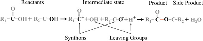
The detachment of LGs (i.e., and ) from two reactants results in corresponding synthons. Then, two synthons (i.e., and ) attract each other to form the target molecule (i.e., ) according to Coulomb’s law. Furthermore, the reaction illustrates that the LGs (i.e., and ) form a side product molecule (i.e., ) since they also exhibit opposite EPs when the target molecule is forming.
These observations inspire us to uncover underlying retrosynthesis rules via Retro-MTGR. Specifically, we reveal why a bond can be the reaction centre via the bond embedding space in Section Bond View. Meanwhile, we explore which LGs are appropriate for generating synthons via the joint embedding space of the LGs and synthons in Section 'Joint View of Synthons and Leaving Groups'.
Bond view
To interpret why a bond can be the reaction centre, we consider the following three bond-derived questions.
-
Can bond energies alone determine the reaction centre in a molecule?
For a chemical bond, its bond energy (i.e., the minimum energy required to break it down) measures its stability44. The greater the bond energy is, the more stable the bond is, and the more difficult the bond is to synthesize from the point of view of chemical retrosynthesis. Thus, we assume that the reaction centre is a low-energy bond.
To validate this hypothesis, we first generate a statistical distribution of the bond energies across all molecular bonds in a histogram (Supplementary Fig. 3). Note that the bond energy used here refers to the theoretical bond energy of the target chemical bond, which is used for two reasons. First, it is challenging to measure real bond energies (e.g., in the gas phase43). Additionally, the bond energy of a bond varies due to the influences of its neighbouring bonds or near atoms in diverse molecular conformations44. Thus, we consider only the theoretical breaking energy of each chemical bond. We collect the theoretical values of the bond energies from the textbook ‘Handbook of chemistry and physics’45. The list of theoretical bond energies can be found in Supplementary Data 1. The bonds are sorted into 20 equally spaced bins along the bond energy axis between the minimum and maximum energy values (kJ/mol). Due to the difference between the numbers of reaction centres and ordinary bonds, the heights of the bins (i.e., the number of bonds falling in the bins) are normalized by the total number of bonds to conduct a convenient comparison.
As illustrated in Supplementary Fig. 3, both the USPTO-50K and USPTO-480K datasets possess similar distributions, and no significant difference is found (p-value = 0.999 under a paired-sample t-test). The underlying reason for this finding is that USPTO-50K guarantees the representativeness of the most common reaction types used in medicinal chemistry43. Overall, most bonds fall into four bins: [270,315], [315, 360], [450-495], and [495-540]. Specifically, the bond energies of reaction centres are usually located in the lower bond energy range (i.e., 95.26% of reaction centres have bond energies <360 kJ/mol). In contrast, 45.33% of the ordinary bonds have bond energies <360 kJ/mol, and 54.65% have bond energies ≥360 kJ/mol. Thus, a naïve decision can be made: bonds with bond energies >360 kJ/mol are usually ordinary bonds.
Such a finding can be used to filter out ordinary bonds with large breaking energies during the reaction centre identification process. This is why bond energies significantly contribute to the identification of reaction centres. However, bond energies cannot determine the reaction centre in a molecule alone since ordinary bonds (45.33%) still overlap with the reaction centres in cases with low breaking energies (<360 kJ/mol). Based on the bond embedding space, this issue can be further investigated by answering the second question.
-
What is the underlying chemical rule captured by bond embeddings such that reaction centres can be distinguished from ordinary bonds?
One of the core contributions of our model (Retro-MTGR) is the discrimination of reaction centres from ordinary bonds in cases with low bond energy. Since bond embedding representations (Formula 4) characterize bond features based on molecular graph topologies, we utilize them to determine the difference between reaction centres and ordinary bonds. Principal component analysis (PCA) is used to visualize bonds in 2-dimensional space, where each point represents a bond.
Such a bond space is rendered (Fig. 3). Figure 3A clearly separates the reaction centres (red points) and ordinary bonds (blue points), except for a small overlapping area. This separation result demonstrates that our model can effectively characterize the difference between reaction centres and ordinary bonds. More importantly, both reaction centres and ordinary bonds can be split into communities, which are strongly specific to bond types. Figure 3B indicates that bond communities are consistent with their bond types. We find that 7 bonds of the same type, namely, C#N (triple bond with a theoretical bond energy of 891 kJ/mol), C#C (triple bond, 837 kJ/mol), c ~ c (aromatic bond, 533 kJ/mol), C = O (double bond, 728 kJ/mol), C = N (double bond, 615 kJ/mol), c ~ n (aromatic bond, 483 kJ/mol), and C = C (double bond, 611 kJ/mol), from unique communities. Commonly, they are ordinary bonds with high bond energies ( > 480 K kJ/mol).
In contrast, single bonds with lower bond energies (<360 kJ/mol) usually fall into two communities, such as C-C, C-c, c-c C’-C’, C’-O’, c-O, C’-N’, and C-S. One of the communities is labelled the reaction centre, and the other is labelled an ordinary bond. As shown in Fig. 3C, a C-C bond is the reaction centre (shown by the brown dashed line) if one of the carbon atoms connects with an oxygen atom via double bonds. Otherwise, it is just an ordinary bond (shown as a solid brown line). Significantly, two types of single bonds (i.e., C-N and C-O) fall into >2 communities. For example, C-O bonds are split into 4 groups, of which 3 groups are annotated as reaction centres, and the remaining group is annotated as an ordinary bond group. As in previous cases, the connection of the carbon atom in a C-O bond with diverse atoms (e.g., oxygen or Cl) is the key to being a reaction centre. Again, the connection of the oxygen atom in a C-O bond with a sulphone group pushes the C-O bond to act as a reaction centre. In contrast, a C-O bond is usually an ordinary bond if its carbon and oxygen atoms have no extra connections beyond alkyl groups or hydrogen atoms (Fig. 3D).
In brief, as illustrated in the bond embedding space, bonds (e.g., double bonds, triple bonds, and aromatic bonds) with high energy (≥360 kJ/mol) are always ordinary bonds and gather in their communities. Moreover, most single bonds with lower bond energies can be reaction centres or ordinary bonds, which are grouped into two or more communities. The local structures around the atoms in bonds determine whether a bond is a reaction centre. In particular, compared with other single bonds, both C-N and C-O bonds are involved in more diverse molecular structures, resulting in >2 reaction centre communities. The details can be found in the Supplementary Data 2.
Why can a bond be the reaction centre in one molecule but not in another molecule?
Fig. 3. Bond space.

A Reaction centres and ordinary bonds. Red dots indicate reaction centres, while blue dots indicate ordinary bonds. B Bond types. Different colours represent different bond types. C C-C bond communities. The left reaction template indicates an ordinary C-C bond while the right shows a reaction centre. D C-O bond communities. The left three reaction templates indicate C-C reaction centres while the right shows an ordinary C-O bond. Regarding the chemical symbols in (B), the symbol C stands for a carbon atom, c denotes a carbon atom in an aromatic bond, and C’ represents a carbon atom in a general ring. Moreover, N stands for a nitrogen atom, n signifies a nitrogen atom in an aromatic bond, and N’ represents a nitrogen atom in a general ring. In addition, O denotes an oxygen atom, O’ represents an oxygen atom in a general ring, and S signifies a sulphur atom. Four specific symbols, including ‘~’, ‘-’, ‘=’, and ‘#’, denote aromatic, single, double, and triple bonds, respectively. In (C) and (D), ‘R1’ and ‘R1’ denote alkyl groups. All atom individuals are numbered while hydrogen atoms are omitted. Reaction centres and ordinary bonds are highlighted by brown dashed lines and brown solid lines respectively. Source data are provided as a Source Data file.
Considering that bond energy cannot determine the reaction centre in a molecule alone, our model (Retro-MTGR) leverages molecular graph topologies to capture the differences between reaction centres and ordinary bonds, even those with the same bond types. We investigate what hidden chemical rule is captured by atom/bond embeddings. It is anticipated that this inherent law will help identify reaction centres and ordinary bonds, especially in cases with both common bond types and similar bond energies.
Our investigation is inspired by the chemical knowledge that the electrical property (denoted as p) of an atom in a molecule is determined by the conjugation effect of the motion of its electrons as well as the union of its spatially neighbouring atoms. When exhibiting an attractive impact on electrons, the examined atom is considered an electron-withdrawing atom. Otherwise, it is called an electron-donating atom. Since it is challenging to quantify the EPs of atoms due to complicated interatom influences, we first propose a qualitative method for determining the strengths and weaknesses of these materials based on expert knowledge. Then, when enumerating atom-centred substructures, we identify 356 substructures, which are categorized into four groups in terms of their EP strengths. Specifically, the atoms showing exhibiting electron-withdrawing/donating properties are labelled p++ and p−−, respectively. Furthermore, the atoms exhibiting weak electron-withdrawing/donating properties are denoted as p+ and p−, respectively. As a result, the atom pairs forming bonds show ten possible pairs of EPs (e.g., (p++ | p−−) and (p+| p−)) in total.
First, we count the percentages of all types of EP pairs in the case involving both reaction centres and ordinary bonds (Supplementary Fig. 4). This observation illustrates that the atom pairs that form reaction centres have opposite dominant EPs (97.0% with ‘p+| p−’, ‘p+|p−−’, ‘p++ | p−’, and ‘p++ |p−−’ pairs), while those pairs that form ordinary bonds have the same or similar EPs (80.1%). Some ordinary bonds with opposite EPs are also reaction centres in the deeper steps of the retrosynthesis process. See also Section Case Study.
To validate whether our bond embeddings can capture the underlying rule, we form an EP distribution of the atom pairs in bonds w.r.t. the bond embeddings of the training dataset. Specifically, the bond embeddings are first mapped to one-dimensional values by an MLP. Then, a histogram EP plot is drawn (Fig. 4), where the horizontal axis indicates the values of the 1-D bond embeddings and the vertical axis indicates the proportion of bonds falling into specific bins of bond embedding values. Moreover, we illustrate a set of histograms produced w.r.t. pairwise EP patterns, where four patterns account for reaction centres and six patterns account for ordinary bonds (Supplementary Fig. 5). In conclusion, all these histograms show that bonds with opposite EPs tend to have larger bond embedding values, and vice versa. Therefore, our bond embeddings reflect the underlying EPs.
Fig. 4. Electrical property distributions of the atom pairs contained in bonds.
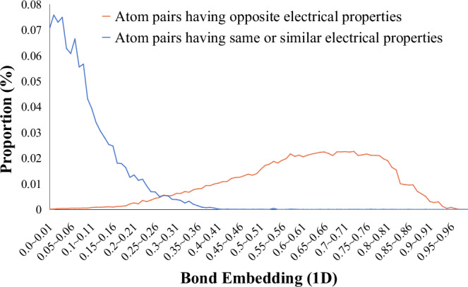
The total number of atom pairs is 274,389, where the number of atom pairs having opposite electrical properties is 78,666 and that of atom pairs having same or similar electrical properties is 195,723. The horizontal axis indicates the values of 1-D bond embeddings, while the vertical axis indicates the proportions of bonds falling into specific bins of bond embedding values. Source data are provided as a Source Data file.
Finally, from the viewpoint of EPs, we review the cases with low bond energy from the previous section (Fig. 3C). When a C-C bond is a reaction centre, except for alkyl groups (R-groups) or hydrogen atoms, its carbon atom connects with an extra oxygen atom, which causes two carbons in the bond to have opposite EPs. Specifically, the left panel shows that both the electronegativity of the oxygen atom and its conjugated double bond with the No. 2 carbon atom cause the electron-withdrawing property of the No. 2 carbon atom. Moreover, the R2 group results in the electron-donating property of the No. 3 carbon atom. Thus, the No. 2 and No. 3 carbon atoms have opposite EPs. In contrast, in the right panel, since the No. 1 and No. 2 carbon atoms have similar EPs, the C-C bond is an ordinary bond. A similar reason explains why C-O bonds are reaction centres or ordinary bonds. In addition to oxygen atoms, halogen atoms connected to carbon atoms and sulphone groups linked to oxygen atoms in C-O bonds cause opposite EPs between the carbon (electron-donating) and oxygen (electron-withdrawing) atoms in C-O bonds.
In brief, the structural difference between the neighbouring bonds of an atom determines its electrical properties. Atom pairs in reaction centres tend to have opposite EPs, while those in ordinary centres tend to have the same or similar EPs.
Thus far, we have leveraged bond embeddings generated by Retro-MTGR to determine why a bond can be a reaction centre by embedding molecule topologies. Bonds with high bond energies are non-single bonds (e.g., double bonds, triple bonds, and aromatic bonds), which are always ordinary bonds. Bonds with lower bond energies are single bonds, which can be reaction centres in some molecules and ordinary bonds in others. A bond is a reaction centre if its member atoms have opposite EPs and is an ordinary bond otherwise. The EP of an atom depends on its neighbouring bonds.
Joint view of synthons and leaving groups
The LGP in Retro-MTGR enables the construction of a joint embedding space for synthons and LGs that helps interpret which LGs are appropriate for particular synthons. For a vivid visualization, we map the high-dimensional embedding space to its 3D form via PCA (Fig. 5). In this space, we consider the following four questions.
-
What is the association between the two synthons in a reaction?
As observed, synthons exhibit a valley-shaped surface, where blue and red points account for synthons possessing positive EPs and negative EPs (denoted as and ), respectively. Several crucial characteristics of synthons can be found. First, their projecting plane expanded by the first two principal components (PCs) illustrates a considerable degree of separation between and even with just the first principal component (PC1). For example, 94.61% of synthons can be correctly separated at PC1 = −0.375, where and tend to have smaller and larger PC1 values, respectively (Fig. 5B). Moreover, the average distances of the synthons in the same reactions and those of the synthons in different reactions are investigated. As illustrated in Fig. 6A, the comparison shows that the former average distance (3.609 ± 1.47) is significantly greater than the latter distance (2.683 ± 1.49) according to a univariate analysis of variance (p-value = 0.0059 < 0.05). Overall, the embedding space illustrates that two synthons in the same reaction always have opposite EPs and are distant from each other, and vice versa.
-
What is the association between a synthon and an LG in a reactant?
More importantly, LGs with positive EPs (denoted as and marked by triangles) also exhibit separation from LGs with negative EPs (denoted as and marked by circles) along with the first principal component in terms of EPs (Fig. 5B). For example, 77.05% of the LGs can be correctly distinguished even with just a linear separation at the position of PC1 = −0.375, where and tend to have larger and smaller PC1 values, respectively, than synthons. Furthermore, tends to occur in the zone, while tends to appear in the zone. To determine the underlying association between synthons and LGs, we calculate the distance between a synthon and an LG in the same reactant () and that between a synthon and an LG in different reactants (). As shown in Fig. 6B, (1.22 ± 0.82) for the same reactants is significantly lower than (2.59 ± 1.15) for different reactants according to a univariate analysis of variance (p-value = 0.0082 < 0.05). In general, the embedding space illustrates that a synthon and an LG tend to form a reactant if they are close to each other and follow the matching rule of positive and negative EPs.
-
What is the tendency for LG to occur?
Similar to synthons, LGs also scatter on the valley-shaped surface (Fig. 5A). First, we find that several LGs occur many times, while many LGs occur a few times. The node sizes denotes their occurrence frequencies in Fig. 5. The former are simple groups (e.g., H, OH, or halogens), while the latter are usually chemical substructures. To determine the underlying reason for this finding, we investigate the number of LG occurrences according to different reaction types (Supplementary Data 3). The investigation reveals that LGs can be split into two categories according to the number of reaction types they participate in. The first category, ‘reaction-common’ LGs, contains LGs that appear in equal to or more than half the total number of reaction types (i.e., >3). They are usually simple LGs, occur frequently, and have many matching partner LGs. Specifically, ‘H’, ‘OH’, ‘Cl’, and ‘Br’ appear in 6, 6, 6, and 5 categories, respectively. In particular, ‘H’ is involved in almost all reactions, occurring 27623 times and having 37 kinds of matching partner LGs (denoted by the node degrees in the graph). The embedding space shows that reaction-common LGs with opposite EPs are far from each other. For example, the distances between H and OH, between H and Cl, and between H and Br are 4.74, 4.89, and 4.03, respectively. These distances are greater than the average distance between all pairs of LGs (2.19). This finding is consistent with the statement that an excellent LG tends to be structurally simple (even monatomic) and to exhibit strong electron affinity and lower bond dissociation energies (e.g., H, Cl, Br, and OH)40. The second category, named ‘reaction-specific’ LGs, includes LGs occurring only in specific types of reactions. They are usually composed of chemical substructure groups, such as ‘-CC’, ‘-OCC(Cl)(Cl)Cl’, and ‘-OCC(F)(F)F’. Reaction-specific LGs gather into clusters on the valley-shaped surface. Some clusters contain many reaction-specific LGs. For example, in the case with 16 LGs exclusively occurring in Type-2 reactions, the average distance within Type-2 reactions (0.82) is less than that of all the LGs (2.19). Similarly, the average distance of LGs exclusively occurring within Type-3 reactions is 1.31. Usually, LGs involved in the same type of cluster have similar chemical structures, such as ‘CCOC( = O)O’ and ‘CC(C)(C)OC( = O)O’ in Type-2 reactions (0.783) and ‘B1OCCO1’ and ‘B1OCCCO1’ (0.754) in Type-3 reactions, where the similarity is calculated by MACCS fingerprints in terms of Jaccard similarity. The chemical structural similarity of LGs implies their potential for substitution, which is determined by costs or the reaction conditions available in synthesis reaction routes. In addition, each of several clusters contains one or a couple of reaction-specific LGs; these occur only a few times and tend to be near reaction-common LGs having the same EPs or far from reaction-common LGs possessing opposite EPs. For example, ‘CCC[SnH](CCC)CCC’, which has negative EPs and occurs 1 time, is near ‘OH’ (distance = 0.61) but far from ‘H’, which has a positive EP in the embedding space (distance = 4.96). In total, reaction-common LGs tend to spread widely, while reaction-specific LGs tend to gather w.r.t. their reaction types and tend to be clustered similarly in terms of structure. In addition, the LGs are rendered in terms of their reaction types in the LGCoG to provide a clear visualization (Fig. 7A).
What is the association between two LGs in a reaction?
Fig. 5. Embedding space of synthons and LGs.

A 3D embedding space. B PC1-PC2 plane. C PC2-PC3 plane. D PC1-PC3 plane. For simplicity, the electron-withdrawing property is denoted as a positive EP (+), while the electron-donating property is denoted as a negative EP (−). Synthons with positive EPs and negative EPs (denoted as and ) are rendered as blue and red points, respectively. LGs possessing positive EPs and negative EPs (denoted as and ) are marked by triangles and circles, respectively. In addition, the marker sizes represent LG occurrence frequencies (degrees), while the filled colours account for the types of reactions where LGs occur. Source data are provided as a Source Data file.
Fig. 6. Distance distributions.
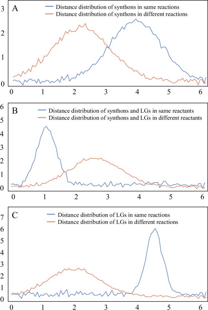
A Pairwise distance distributions between synthons. The blue line represents the distance distribution of synthons presenting in the same reactions, while the red line represents that of synthons in different reactions. B Pairwise distance distributions between synthons and LGs. The blue line represents the distance distribution of synthons and LGs belonging to the same reactants, while the red line represents the distribution in the case with different reactants. C Distance distributions between LGs in the embedding space. The blue line represents the distance distribution of LGs co-occurring in the same reactions, while the red line represents the distribution of LGs in different reactions. The comparisons in (A), (B) and (C) demonstrate the significant difference between two distance distributions under a univariate analysis of variance with p-value = 0.0059, p-value = 0.0082 and p-value = 0.0014 respectively. Source data are provided as a Source Data file.
Fig. 7. LG view.

A Reaction type map. LGs occurring in single reaction types, multiple reaction types (≤3), and many types (>3, reaction-common) are highlighted in different colours. B EP map. LGs with positive and negative EPs are rendered in blue and red, respectively.
Finally, we consider the occurrence of LG pairs. Overall, 94.3% of the LG pairs in the same reactions have opposite EPs, which cause two LGs in a reaction to be apart from each other in the embedding space. In particular, we investigate the pairwise distances between the LGs in the embedding space. Figure 6C shows that the pairwise distances between co-occurring LGs (3.92 ± 0.99) in reactions are greater than those between non-co-occurring LGs (2.14 ± 1.11) according to a univariate analysis of variance (p-value = 0.0014 < 0.05). Specifically, we find that LG pairs consisting of two simple groups (e.g., H, OH, or halogens) usually occur frequently. In particular, the pairs ‘H, OH’ (27.8%), ‘H, Cl’ (27.4%), ‘H, Br’ (12.9%), and ‘H, I’ (8.1%) are the most frequent LG pairs. Moreover, LG pairs including simple groups and chemical substructures, such as ‘Br, CC1(C)OBOC1(C)C’ (1.8%), occur at low frequencies. Few LG pairs (0.386%) are composed of chemical substructures only, such as ‘O = S( = O)(O)C(F)(F)F-B(OH)2, O = S( = O)(O)C(F)(F)F-CC1(C)OBOC1(C)C’. In addition, the LGs are rendered in terms of their EPs in the LGCoG to provide a straightforward visualization (Fig. 7B). Thus, the embedding space illustrates that the more distant two LGs with opposite Eps are, the greater their co-occurrence, or the more likely they are to have the same reaction.
In summary, the union of synthons and LG co-occurrences results in an embedding space, which captures the underlying association rules between the synthons and LGs. First, the two synthons in a reaction always have opposite EPs and are distant from each other in the embedding space. Second, a synthon and an LG belonging to a reactant usually have opposite EPs and are close to each other in the embedding space. Finally, two LGs co-occurring in a reaction regularly have opposite EPs and are distant from each other. Therefore, the union of synthons and the co-occurrence graphs of LGs contains rich retrosynthesis information, including the intra-associations between synthons, the inter-associations between LGs and synthons, and the intra-associations between LGs. Our Retro-MTGR method can capture such rich information to achieve an enhanced retrosynthesis prediction effect.
Case study
To evaluate the retrosynthesis prediction ability of our Retro-MTGR method in a real scenario, we collect two drugs (i.e., Sonidegib53 and Acotiamide54) that are not included in our dataset as the study cases. We infer their retrosynthesis routes with Retro-MTGR and then validate them via chemical assays.
The two selected drugs are briefly summarized as follows. The first drug, Sonidegib, is a Hedgehog signalling pathway inhibitor (via smoothened antagonism) that was developed as an anticancer agent by Novartis and approved by the FDA in 2015 for treating basal cell carcinoma. Currently, it is commonly used for the treatment of locally advanced recurrent basal cell carcinoma (BCC) following surgery and radiation therapy or in cases where surgery or radiation therapy is not appropriate (DrugBank ID: DB09143)52. The second drug, Acotiamide, is a medication manufactured and approved in Japan for treating postprandial fullness, upper abdominal bloating, and early satiation due to functional dyspepsia. It acts as an acetylcholinesterase inhibitor (DrugBank ID: DB12482) 53.
Since Retro-MTGR is a single-step retrosynthesis prediction model, we iteratively apply it to infer a complete retrosynthesis route for a given drug molecule. In the first iteration, Retro-MTGR splits the complete molecule into two synthons under the top-1 criterion (the first candidate reaction centre), which are further converted into smaller intermediate molecules by appending appropriate LGs. The intermediate molecules are then split into smaller molecules by Retro-MTGR in a similar manner unless the intermediate molecules are reactants that can be easily bought on the market.
The prediction results of Sonidegib are shown in Fig. 8A. The predicted retrosynthesis route of Sonidegib (marked as ‘1’) illustrates that it can be split into two intermediate molecules (marked as ‘2’ and ‘3’). Furthermore, they are split into two pairs of reactants, where one pair is marked as ‘4’ and ‘5’ and the other is marked as ‘6’ and ‘7’. In each retrosynthesis step, the attention scores of the bonds are labelled, and the highest (top-1) score is considered the reaction centre. During the retrosynthesis route prediction process, both the reaction centres and LGs are correctly predicted.
Fig. 8. Predicted retrosynthesis routes and real chemical synthesis routes.

A Retrosynthesis prediction route of Sonidegib. Sonidegib (‘1’) is split at the reaction centre into intermediate molecules ‘2’ and ‘3’, where the highest attention score generated by our Retro-MTGR method is highlighted. Then, ‘2’ and ‘3’ are further decomposed into four reactants (‘4’, ‘5’, ‘6’ and ‘7’) according to their reaction centres. B Chemical synthesis route of Sonidegib. First, the Suzuki cross-coupling reaction between ‘4’ and ‘5’ is executed to obtain intermediate molecule ‘2’. Furthermore, ‘6’ is converted to ‘8’ with the help of m-Chloroperbenzoic acid (m-CPBA) to prevent its intrareaction. Then, ‘8’ is combined with ‘7’ in the presence of DIEA (N, N-diisopropylethylamine) to form another intermediate molecule ‘9’, which is further reduced by H2 in the presence of Pd/C to generate ‘3’. In the last step, the coupling of compound ‘2’ with ‘3’ in the presence of HATU (2-(7-Azabenzotriazol-1-yl)-N, N, N’, N’-tetramethyluronium hexafluorophosphate) and DIEA (N, N-Diisopropylethylamine) in DMF (N, N-Dimethylformamide) generates Sonidegib (‘1’). C Retrosynthesis prediction route of Acotiamide. Acotiamide (‘10’) is split at the reaction centre into intermediate molecules ‘11’ and reactant ‘12’, where the highest attention score generated by our Retro-MTGR method is highlighted as well. Then, ‘11’ is further decomposed into two reactants (‘13’ and ‘14’) according to their reaction centres. D Chemical synthesis route of Acotiamide. First, reactant ‘14’ is esterified with methanol to form ‘15’. Then, compound 13 is coupled with 15 in the presence of HATU and DIEA to obtain intermediate molecule ‘16’, which is sequentially hydrolysed to another intermediate molecule ‘11’ by NaOH and HCl. Finally, the coupling between the intermediate molecule ‘11’ and the reactant ‘12’ in the presence of HATU and DIEA in DMF generates the Acotiamide molecule (‘10’). More details (e.g., reaction conditions and instruments) about the above chemical synthesis reactions can be found in Supplementary Note 1. Note: DIEA, HATU, m-CPBA, and Pd/C are catalysts used in the abovementioned chemical reactions.
The chemical synthesis assay of Sonidegib is shown in Fig. 8B. Furthermore, according to the prediction results, a series of chemical synthesis reactions starting from reactants (‘4’, ‘5’, ‘6’, and ‘7’) is performed to validate the predicted retrosynthesis route. Remarkably, due to the potential intrareaction among the ‘6’ molecules triggered by their chlorine (-Cl) and amino groups (-NH2), the expected reaction between ‘6’ and ‘7’ generates fewer ‘3’ molecules. To guarantee a high production rate of ‘3’ in the real synthesis process, we convert ‘6’ to ‘8’ with a nitration reaction, which alters the amino group to a nitro group (-NO2). Then, the reaction of ‘8’ and ‘7’ produces ‘9’, where the nitro group is further converted back into the amino group in a reduction reaction to obtain ‘3’ with the desired product. Moreover, the reaction of ‘4’ and ‘5’ generates ‘2’. Finally, we perform an amidation reaction by combining ‘2’ and ‘3’ to form the product molecule Sonidegib (‘1’).
The prediction results of Acotiamide are shown in Fig. 8C. Similarly, the retrosynthesis route of Acotiamide (marked as ‘10’) is correctly predicted in terms of both its reaction centres and LGs and validated by chemical synthesis reactions. Specifically, the first retrosynthesis step generates an intermediate molecule (‘11’) and a reactant (‘12’). Then, the former molecule is split into two reactants (‘13’ and ‘14’) in the second step.
The chemical synthesis assay of Acotiamide is shown in Fig. 8D. Since an intrareaction issue is also encountered in ‘14’, a similar strategy is adopted to guarantee the final production of ‘10’. In brief, the carboxylic acid group (-OH) of ‘14’ is altered to a methoxy group (-OCH3) to generate ‘15’ through an esterification reaction. As with the substitution of ‘14’, ‘15’ is combined with ‘13’ to generate a new intermediate molecule, ‘16’, which is sequentially hydrolysed to an intermediate molecule ‘11’ by both NaOH and HCl. Finally, a similar amidation reaction combining ‘11’ and ‘12’ is performed to form Acotiamide (‘10’).
To summarize, the ability of Retro-MTGR to predict retrosynthesis routes is consistent with chemical assays. Thus, this study can provide clear guidance for performing retrosynthesis route planning under extra reaction conditions.
Discussions
Aiming at developing a highly interpretable discriminative model to uncover chemical synthesis mechanisms, this paper presents a Retro-MTGR framework. Based on molecular graphs, three related tasks are simultaneously considered in Retro-MTGR, where two major supervised discriminative tasks account for recognizing reaction centres and identifying LGs, and an auxiliary self-supervised task accounts for generating better atom embeddings.
First, a comparison with 16 state-of-the-art methods demonstrates the superiority of Retro-MTGR. Additionally, its robustness and scalability are validated by different training-testing strategies and datasets of different sizes in both RTU and RTK scenarios.
Then, an ablation study demonstrates the contributions of its modules to the prediction process, as follows. (1) As the most crucial module in Retro-MTGR, the multitask learning framework learns an RCP and the LGP simultaneously to comprehensively characterize synthesis reactions from their reaction centres to LGs, including the bond energy tendencies in reaction centres, the occurrence tendencies of LGs, and the associations between chemical entities in synthesis reactions. (2) An LGCoG, which plays the second-most crucial role in Retro-MTGR, captures both the individual occurrence tendencies and co-occurring associations of LGs. (3) An AEE based on GCL, which plays the third-most crucial role, enhances atom embeddings by leveraging chemical structural redundancy and the differences between a molecule and its synthons. (4) Bond energy, even when working as a single dimension, provides a nontrivial contribution to bond embeddings since bonds with high energies tend to be ordinary bonds. (5) Two numeric tricks (i.e., the utilization of dense atom representations and the elimination of large absolute co-occurrence variances) enable a better learning effect.
More importantly, multiple comprehensive investigations validate the interpretability of the chemical synthesis process of Retro-MTGR by answering two questions: why can a bond be the reaction centre, and what LGs are appropriate for a given synthon? The results demonstrate that Retro-MTGR can capture and illustrate the underlying chemical synthesis rules.
Specifically, the embedding space of bonds illustrates why a bond can be the reaction centre or not based on both USPTO-50K and USPTO-480K. (1) Bonds (e.g., double bonds, triple bonds, and aromatic bonds) with high energy (≥360 kJ/mol) are always ordinary bonds and fall into unique communities. (2) Most single bonds with lower bond energies ( < 360 kJ/mol) usually fall into two communities (reaction centres and ordinary bonds). (3) Two types of single bonds (i.e., C-N and C-O) with lower bond energies ( < 360 kJ/mol) fall into >2 communities due to the diverse molecular structural topologies of their corresponding synthons. (4) The EP distributions of the atom pairs contained in bonds demonstrate that a bond is the reaction centre in a molecule if its member atoms tend to have opposite EPs (as reflected by their local substructures); otherwise, it is an ordinary bond.
Moreover, the joint embedding space of synthons and LGs is appropriate for generating synthons because of the associations between chemical entities. In the embedding space, (1) two synthons in a reaction always have opposite EPs and are distant from each other; (2) a synthon and an LG belonging to a reactant usually have opposite EPs and are close to each other; (3) two LGs co-occurring in a reaction regularly have opposite EPs and are distant from each other; and (4) reaction-common LGs tend to spread widely and are occurrence-dominant, monatomic or structurally simple (e.g., H, Cl, Br, I, and OH), while reaction-specific LGs tend to gather w.r.t. their reaction types and are similar to each other in terms of structures. In addition, occurrence-dominant LG pairs always consist of two simple groups (e.g., ‘H, OH’, ‘H, Cl’, and ‘H, Br’).
Finally, the practical capabilities of Retro-MTGR are evaluated in cases involving two novel drugs. The results reveal that the retrosynthesis routes inferred by Retro-MTGR are consistent with those achieved by chemical synthesis assays. In brief, our Retro-MTGR approach can provide prior guidance for retrosynthesis route planning.
However, the widespread application of Retro-MTGR still faces the following limitations. We believe that an extended version of Retro-MTGR with the integration of additional synthetic factors (e.g. reaction yields, conditions, and reagents) can be a multistep retrosynthesis route planning strategy for the future.
Imbalanced LGs. An extreme imbalance is observed among diverse LGs in terms of occurrence. For example, ‘H’ occurs 27624 times, while ‘CCCCCCCCCCCCO’ occurs only once in USPTO-50K. Although the individual occurrence tendencies of LGs assist with the LGP task, Retro-MTGR has insufficient training data for minority LGs, resulting in bias towards the majority LGs. Generative algorithms (e.g., autoregressive models and generative adversarial networks) are promising approaches for generating more reactions involving the minority LGs to address this issue. Moreover, since the list of all possible LGs is enumerated from the training data, some LGs in the testing dataset are not fully covered. Retro-MTGR is at risk of failing in these cases. It is feasible to build a list of LGs with high coverage based on a larger dataset (e.g., USPTO-Full or PubChem).
Incomplete multistep retrosynthesis. Retro-MTGR provides a core single-step retrosynthesis prediction tool and even an initial multistep retrosynthesis route by iteratively decomposing the scaffold of a product into commercial reactants. However, Retro-MTGR only accounts for popular broad-sense coupling reactions (generating one product molecule from two reactant molecules) and can’t modify atoms in branches or small functional groups. The latter case involves four types of minority reactions, including deprotection, protection, reduction, and oxidation reactions. Although not need to modify molecule scaffolds, they play untrivial roles (e.g. increasing yield rate and raw material availability) in multistep retrosynthesis. Therefore, Retro-MTGR should be extended to cover these reactions to attain a complete multistep retrosynthesis planning effect.
Lack of real bond energies. Similar to atom properties and bond types, theoretical bond energies are easily collected and surely improve bond embeddings. Although they are defined as the standard enthalpy changes exhibited by reactions, bond energies are limited in reflecting the real circumstances of reactions. The appropriate measurement of real bond energies, especially moderate energies, would yield improved bond embeddings.
Lack of numerical EPs. Our results demonstrate that the opposition of EPs plays an essential role in determining the interactions between reaction sites and LGs. Nevertheless, we are currently limited to personal expert experience for qualitatively estimating EPs. We believe that assay-determined quantitative EPs would significantly improve the effects of retrosynthesis prediction.
Methods
Problem formulation and model construction
Given a set of chemical reactions , the task is to find a retrosynthesis strategy for a newly designed target molecule (i.e., to recommend reactants for ), where the reactants and are two reactant molecules for the synthesis of the target molecule . Remarkably, this task only focuses on the reactions involved in the scaffold decomposition process of the target molecule (i.e., broad-sense coupling reactions), which is the core of retrosynthesis planning. However, reactions (e.g., deprotections, protections, reductions, and oxidations), which involve modifying atoms in branches or bonds in small functional groups, are discarded.
To implement a chemist-like retrosynthesis process, we develop a Retro-MTGR framework, which contains an RCP module, an AEE module and an LGP. They account for two major tasks and one auxiliary task. The first major task, implemented by the RCP, is modelled as a binary discrimination problem, which recognizes the reaction centre among all the bonds of the target molecule. Additionally, is broken down to obtain two synthons and , where are two bonding atoms in . To support the first major task in terms of the associated atom embeddings, the auxiliary task (implemented by the AEE) is modelled as a self-supervised contrastive learning problem that characterizes the structural commonalities and differences between and its synthons . The second major task is modelled as a multiclass discrimination problem that assigns appropriate LG to the synthons to form complete reactants under enhanced LG dependence. All the symbols used are listed in Supplementary Table 7.
Reaction centre predictor
Reaction centre identification is the first step in the retrosynthesis inference process. Inspired by the existing semi-template-based approaches, we primarily attempt to recognize the reaction centre among all the bonds of a given target molecule. In retrosynthesis, the bond at the reaction centre is broken. Thus, the task of reaction centre recognition can be naturally modelled as a binary discrimination problem, which recognizes the reaction centre among all the bonds of the target molecule.
For this task, we design an RCP module, which includes an atom encoder, a bond-level readout layer, and a multilayer perceptron (MLP). The atom encoder is implemented by a multilayer MPNN to convert molecular graphs into atom embeddings , which are further refined by an AEE. The bond-level readout layer generates bond embeddings , which are further boosted by concatenating them with bond energy and bond type embeddings . The MLP accounts for the discrimination of bonds through , where if is the reaction centre and otherwise.
Atom encoder
According to its chemical structure, each compound is represented as a molecular graph , where is the set of its atoms, is the set of its bonds , and . Let be its adjacency matrix, in which indicates the bond occurring between two atoms (i.e., and ) and indicates the lack of a bond. Suppose that is the initial feature vector of atom , which is usually coded into a vector containing one-hot-shaped atom types, the number of hydrogen atoms, and other attributes55. Usually, the one-hot encoding attributes in are sparse, while other attributes are dense (e.g., nonzero integers (numbers) of atom or degrees). Thus, is partially sparse or semi-sparse. An extra MLP maps it to a dense form () to learn better embeddings, as suggested by Cheng et al.51
Both and are input into a multilayer MPNN to generate atom embeddings for molecule . The MPNN updates the embedding of each atom by aggregating those of its neighbouring atoms in a layer as follows:
| 1 |
| 2 |
where ‘’ formally represents the vector concatenation operation32, denotes the embedding of atom in the t-th layer of the MPNN, denotes the neighbours of atom in the molecular graph , is a nonlinear activation function (e.g., ), and denotes a learnable bias. Moreover, indicates the weight across the neighbours of , indicates the weight of in , and indicates the weight of w.r.t. layer t. Inspired by Gilmer56 and Kipf57, we believe that the weights ‘’ are specific to different layers. In addition, is the one-hot coding vector of bond types, within which four bits denote the presence of single bonds, double bonds, triple bonds, and aromatic bonds. In short, the atom embedding update rules are defined as follows:
| 3 |
Bond-level readout
After passing through the MLP and the MPNN in order, the initial feature vector of atom is mapped to its p-dimensional dense representation and its embedding in turn. Then, the atom embeddings are further refined by the AEE module, which characterizes the structural commonalities and differences between the molecule and its synthons. This embedding is used by RCP to identify the reaction centre. Meanwhile, it is utilized by the LGP module to help find appropriate leaving groups for the synthons. All three tasks are associated together by shared atom embeddings.
The refined atom embeddings are subsequently used to generate bond embeddings via the bond-level readout process. Let be the bond connecting atoms and . Unlike the ordinary molecule-level readout method (e.g., combining all atoms), the RCP model defines a bond-level readout function , which is augmented by bond energy because bonds with strong energies tend to be ordinary bonds43. The bond embedding is obtained as follows:
| 4 |
where is the theoretical bond energy and ‘’ indicates the concatenation of atom embeddings and the corresponding bond energy.
Finally, the RCP identifies the reaction centre among all the bonds of . is defined as the set of bond flags w.r.t. molecule , where if is the reaction centre (a positive sample); otherwise, (a negative sample). Based on the abovementioned bond embeddings , an MLP (denoted as ) is constructed as the classifier to achieve such a bond identification effect (i.e., ). To train the model, the cross-entropy loss function calculated over all the training molecules is defined as follows:
| 5 |
where is the set of all the training molecules and is the bond set of .
Atom embedding enhancer
GCL has been applied in diverse areas (e.g., image clustering58, drug-target interaction prediction59, and Parkinsonian assessment60) because it can augment node representations via node dropping, edge perturbation, attribute masking or subgraph extraction42. In particular, recent works on molecular property prediction have demonstrated that molecular GCL (MGCL) can obtain better atom representations and molecular representations than other methods61. As we observed, GCL and retrosynthesis are highly analogous in terms of graph change (regarding a molecular structure as a graph). Inspired by this observation, we designed an AEE module based on GCL to boost atom embeddings.
Our AEE is just an implementation of GCL that involves atom masking, bond deletion, and substructure removal. Akin to the existing GCL methods, our approach determines a contrastive positive sample based on a target molecule (product) and another different molecule. However, unlike these methods, we do not deliberately design contrastive positive samples via bond perturbation (i.e., node connectivity variation). In contrast, we directly use the target molecule (product) and the combination of its two synthons as a contrastive positive sample because the difference (the reaction centre) between the product and its combined synthons naturally plays a role in bond perturbation. The AEE module is expected to augment atom embeddings to better identify reaction centres.
Formally, for a target molecule , we treat its synthons ( and ) as a new perturbed molecule . The ‘perturbation’ concept is taken from Liang et al.62. Perturbed molecules were originally referred to as incomplete molecules generated by randomly removing atoms or bonds from a target molecule63. In our work, the perturbed molecule is specifically defined as the combined structure of two synthons. Compared to , has no reaction centre. During contrastive learning, a positive sample is defined as the pair consisting of and its perturbed molecule since they are nearly the same. In contrast, a negative sample is defined as the pair consisting of and another molecule different from . Here, refers to a molecule randomly selected from the training set. Contrastive learning pushes and as close together as possible while pushing and as far apart as possible, resulting in better atom embeddings.
Let , , and be the respective embeddings of the above molecules. These molecule embeddings are generated by an atom encoder and a molecule-level readout function . The former shares parameters with the atom encoder used in the RCP module. For a given molecule, aggregates the embeddings of all its atoms to generate a molecule-level embedding via average pooling: .
In terms of contrastive learning, the molecule embedding pair of and is regarded as a positive sample, while the pair of and is taken as a negative sample. Our goal is to train a contrastive learning model that pushes and as close together as possible (similar) while pushing and as far apart as possible (different). For this purpose, we design a contrastive loss function as follows:
| 6 |
Thus, the AEE module enables an ingenious process for utilizing the chemical structural commonness and differences between a molecule and its synthons to produce enhanced atom embeddings for other tasks.
Leaving group predictor
Once synthons are determined based on the reaction centre, chemists can obtain the corresponding reactants by attaching appropriate LGs to them. Thus, the LG recognition task can be modelled as a multiclass classification problem. More importantly, we believe that LGs are not independent but rather associated in terms of chemical synthesis. First, an excellent LG tends to be structurally simple (even monatomic) and to exhibit strong electron affinity and lower bond dissociation energies64. Moreover, two LGs in a synthesis reaction are associated since they form the side product (e.g., ) accompanying the target molecule.
Based on these considerations, we propose an elaborate LGP based on multiclass classification to identify LG. Formally, let be the list of all possible LGs, be the reaction centre of molecule , be the reaction sites (i.e., the atoms forming ), and be the corresponding synthons. The task is to assign to an appropriate LG (i.e., ) to form its corresponding reactants (i.e., ), where indicates a mapping function from to . Note that the list of all possible LGs is enumerated from the training data.
To capture the individual occurrence tendencies and co-occurrence associations of LGs, we construct an LG co-occurrence graph (LGCoG) , where denotes the set of nodes (LG) and denotes the set of weighted edges (normalized co-occurrences between the LGs). Each LG is a small chemical substructure (e.g., -OH or -B(OH)2) or an individual atom/ion (e.g., -Cl, -Br, or -H). The popular one-hot coding method is used to determine the initial node features . The edge building process consists of two steps. is defined as the LG co-occurrence matrix, where denotes the number of pairwise co-occurrences between and . The co-occurrence of two LGs is counted if they are involved in the same reaction. For example, the co-occurrence of ‘-H’ and ‘-OH’ is counted once in the reaction . After enumerating all the possible LG pairs, their co-occurrences are counted over all the reactions in the training dataset. Then, a probability matrix can be calculated via . Therefore, is calculated as follows:
| 7 |
Remarkably, the normalization step in Formula (7) should be considered because the values of vary greatly. For example, the co-occurrence between ‘-H’ and ‘-OH’ is 9451, while that between ‘-H’ and ‘-CC( = O)O’ is only 1. Since small co-occurrence values are overwhelmed by large values during training, a trained model with a massive absolute co-occurrence variance would decrease retrosynthesis prediction performance. The ablation study conducted in section results demonstrates the effectiveness of the normalization step.
We set as the weight of the edge from to (i.e., ). Thus, the embedding () of LG can be represented by implementing an MPNN on as follows:
| 8 |
where is a nonlinear activation function (i.e., ReLU), is the neighbourhood of , indicates the weight across the neighbours of LG , indicates the weight of belonging to , and indicates the weight of w.r.t. layer t.
Moreover, inspired by chemists, we believe that the reaction centre and the local substructures around the reaction sites are crucial factors for determining the corresponding LGs. To characterize synthons, the reaction centre is represented by its bond embedding in the RCP, while the local substructure around reaction site is represented by the atom embedding , which already aggregates its neighbours due to the MPNN contained in the RCP. Thus, the embedding of the synthon containing can be defined as their concatenation . Similarly, we can define the embedding of by .
After obtaining the synthon and LG embeddings, we can directly determine the candidate LG that should be attached to a synthon. We assume that in a synthon-LG association, the synthon and LG tend to form a reactant if they are close to each other in their embedding space. As suggested by MLGL-MP65, we measure the proximity between a given synthon and a given LG as follows:
| 9 |
The proximity is the prediction score regarding the attachment of the given synthon to the -th LG in the LG set , and it reflects how likely is to be attached to . It is anticipated that the proximity measure captures the underlying association between synthons and LGs.
However, such a direct proximity measure would be senseless since the synthon embedding and LG embedding spaces are different vector spaces. To address this issue, we design an adaptor to map to . The adaptor can be implemented by an MLP containing an input layer, a hidden layer, and an output layer. Thus, the final compound representation feature is defined as = , where is the dimensionality of . It is remarkable that such an adaptor enables the formation of a joint embedding space for synthons and LGs, where the inter-associations between synthons and LGs, the intra-associations between synthons, and the intra-associations between LGs can be characterized simultaneously.
Finally, the mean squared error (MSE) loss function is used when training the LGP as follows:
| 10 |
where is the true label indicating whether a synthon is attached to an LG , is the corresponding score output by the LGP, is the total number of training molecules, and represents the number of corresponding synthons.
Training loss and testing
To learn the bond energy tendencies of reaction centres, the occurrence tendencies of LGs, and the associations between chemical entities in synthesis reactions, we simultaneously train the reaction centre recognition and LG identification modules under the framework of multitask learning66,67. During training, Retro-MTGR learns three related tasks, including two major tasks (reaction centre recognition and leaving group prediction) and one auxiliary task (atom embedding enhancement via GCL). Accordingly, we jointly optimize the three loss functions formed w.r.t. these tasks into a linear combination as follows:
| 11 |
where denotes the normalized hyperparameters for adjusting the task weights. The tuning process for finding the optimal values of can be found in Supplementary Fig. 2.
Notably, the training process of Retro-MTGR is different from its testing procedure because the contrastive learning-based AEE should be removed from the testing process. A similar strategy can be found in Liu et al.68. Technically, the training process of Retro-MTGR involves the atom encoder, AEE, RCP, and LGP modules. After training, a set of neural networks is constructed, including the MLP and the MPNN in the atom encoder, the MLP in the RCP, and the adaptor and the MPNN in the LGP. Note that the AEE contains no neural network but instead has a molecule-level readout and a contrastive loss, which help obtain better atom embeddings during training. During the testing process performed for a given target molecule, Retro-MTGR leverages the trained neural networks in the atom encoder, RCP, and LGP modules to determine its reaction centre and the LGs of its two synthons.
Performance metrics
To measure the retrosynthesis prediction effects of the tested methods, we adopt the top-k accuracy, which is a prediction metric that is popularly used in the existing works32,38.
Technically, for a given target molecule, the trained model (i.e., Retro-MTGR) infers the bond candidates for its reaction centre, which are ordered by their prediction scores. A higher score indicates a greater probability of the corresponding bond candidate being the reaction centre. After ranking the bond candidates, we pay attention to the first k bond candidates, such as the top-1, top-3, and top-5 results. Furthermore, each bond candidate accounts for a pair of synthons, which are assigned two LGs to form a predicted reactant pair. Here, Retro-MTGR provides predictions for only the top-1 LGs. Thus, we obtain the top-k predicted reactant pairs based on the top-k bond candidates. Among the top-k predicted reactant pairs, a pair of reactants is counted as a correct prediction if they are the same as the real reactants of the target molecule. In this case, we regard the target molecule as a correctly predicted sample in terms of the top-k prediction process. Therefore, the top-k accuracy is defined as the ratio of the number of correctly predicted target molecules out of top-k predicted candidates to the total number of target molecules.
Model implementation details
Model trainings use the Adam optimizer for gradient descent optimization with an initial learning rate set to 0.01. The training process lasted approximately 73.5 h (USPTO-50K). All experiments were conducted on a hardware setup comprising four NVIDIA A800 GPUs (each with 64 GB memory) and an Intel Xeon Gold 6348 CPU @ 2.60 GHz.
Reporting summary
Further information on research design is available in the Nature Portfolio Reporting Summary linked to this article.
Supplementary information
Description Of Additional Supplementary File
Source data
Acknowledgements
This work was supported by the National Natural Science Foundation of China (62372375 J.Y.S.), the Shaanxi Province Key R&D Program (2023-YBSF-114 J.Y.S.), the CAAI-Huawei Mind Spore Open Fund (CAAIXSJLJJ-2022-035A J.Y.S.), and the Scientific and Technological Innovation Project of China Academy of Chinese Medical Sciences (CI2023C065YLL C.L.).
Author contributions
P.Z., X.W., and J.Y.S. designed the research. P.Z., X.W., Q.W., and Q.H.W. handled the data processing. J.L. and J.S. evaluated the performance of single-step retrosynthesis. P.Z. and J.Y.S. conducted the experiments. P.Z., C.L., and J.Y.S. wrote the manuscript. P.Z., C.L., J.S., and J.Y.S. revised the manuscript. All authors reviewed and approved the final manuscript.
Peer review
Peer review information
Nature Communications thanks the anonymous, reviewer(s) for their contribution to the peer review of this work. A peer review file is available.
Data availability
We used the benchmark datasets USPTO-50K, USPTO-MIT, and USPTO-FULL for all our experiments. For a fair comparison, we used the same version and splits as those provided by Yan et al.36 for USPTO-50K and USPTO-FULL. The USPTO-MIT dataset is provided by Chen et al.16. The source data can be found at 10.5281/zenodo.1434632469. Source data are provided with this paper.
Code availability
All code of the manuscript, alongside a description of necessary steps for reproducing results, can be found in a GitHub repository accompanying this manuscript: https://github.com/zpczaizheli/Retro-MTGR69. Additionally, the source code is also available at Zenodo repertory through 10.5281/zenodo.1434632469.
Competing interests
The authors declare no competing interests.
Footnotes
Publisher’s note Springer Nature remains neutral with regard to jurisdictional claims in published maps and institutional affiliations.
Contributor Information
Jie Shang, Email: shangjie03@nwpu.edu.cn.
Cheng Lu, Email: lv_cheng0816@163.com.
Jian-Yu Shi, Email: jianyushi@nwpu.edu.cn.
Supplementary information
The online version contains supplementary material available at 10.1038/s41467-025-56062-y.
References
- 1.Zhao, P. et al. Targets preliminary screening for the fresh natural drug molecule based on Cosine-correlation and similarity-comparison of local network. J. Transl. Med.20, 67 (2022). [DOI] [PMC free article] [PubMed] [Google Scholar]
- 2.Li, J. N., Yang, G., Zhao, P. C., Wei, X. X. & Shi, J. Y. CProMG: controllable protein-oriented molecule generation with desired binding affinity and drug-like properties. Bioinformatics39, i326–i336 (2023). [DOI] [PMC free article] [PubMed] [Google Scholar]
- 3.Du, B.-X., Xu, Y., Yiu, S.-M., Yu, H., Shi, J.-Y. MTGL-ADMET: A Novel Multi-task Graph Learning Framework for ADMET Prediction Enhanced by Status-Theory and Maximum Flow. In: Research in Computational Molecular Biology: 27th Annual International Conference, RECOMB 2023, Istanbul, Turkey, April 16–19, 2023, Proceedings (Springer, 2023).
- 4.Gupta, R. et al. Artificial intelligence to deep learning: machine intelligence approach for drug discovery. Mol. Divers25, 1315–1360 (2021). [DOI] [PMC free article] [PubMed] [Google Scholar]
- 5.Vatansever, S. et al. Artificial intelligence and machine learning-aided drug discovery in central nervous system diseases: State-of-the-arts and future directions. Med. Res. Rev.41, 1427–1473 (2021). [DOI] [PMC free article] [PubMed] [Google Scholar]
- 6.Lee, A. A. et al. Molecular transformer unifies reaction prediction and retrosynthesis across pharma chemical space. Chem. Commun.55, 12152–12155 (2019). [DOI] [PubMed] [Google Scholar]
- 7.Dong, J., Zhao, M., Liu, Y., Su, Y., Zeng, X. Deep learning in retrosynthesis planning: datasets, models and tools. Brief Bioinform,23, bbab391 (2022). [DOI] [PubMed]
- 8.Coley, C. W., Green, W. H. & Jensen, K. F. Machine learning in computer-aided synthesis planning. Acc. Chem. Res51, 1281–1289 (2018). [DOI] [PubMed] [Google Scholar]
- 9.Jiang, Y. et al. Artificial intelligence for retrosynthesis prediction. Engineering25, 32–50 (2023). [Google Scholar]
- 10.Yan, M. & Baran, P. S. Drug discovery: fighting evolution with chemical synthesis. Nature533, 326–327 (2016). [DOI] [PubMed] [Google Scholar]
- 11.Jiang, Y., Ying, W., Wu, F., Huang, Z., Kuang, K., Wang, Z. Learning chemical rules of retrosynthesis with pre-training. In: Proceedings of the AAAI Conference on Artificial Intelligence) (2023).
- 12.Coley, C. W., Rogers, L., Green, W. H. & Jensen, K. F. Computer-Assisted Retrosynthesis Based on Molecular Similarity. ACS Cent. Sci.3, 1237–1245 (2017). [DOI] [PMC free article] [PubMed] [Google Scholar]
- 13.Dai, H., Li, C., Coley, C., Dai, B., Song, L. Retrosynthesis prediction with conditional graph logic network. Advances in Neural Information Processing Systems 32 (NeurIPS, 2019).
- 14.Segler, M. H. S. & Waller, M. P. Neural-symbolic machine learning for retrosynthesis and reaction prediction. Chemistry23, 5966–5971 (2017). [DOI] [PubMed] [Google Scholar]
- 15.Baylon, J. L., Cilfone, N. A., Gulcher, J. R. & Chittenden, T. W. Enhancing retrosynthetic reaction prediction with deep learning using multiscale reaction classification. J. Chem. Inf. Model59, 673–688 (2019). [DOI] [PubMed] [Google Scholar]
- 16.Chen, S. & Jung, Y. Deep retrosynthetic reaction prediction using local reactivity and global attention. JACS Au1, 1612–1620 (2021). [DOI] [PMC free article] [PubMed] [Google Scholar]
- 17.Seidl, P. et al. Improving few- and zero-shot reaction template prediction using modern Hopfield networks. J. Chem. Inf. Model62, 2111–2120 (2022). [DOI] [PMC free article] [PubMed] [Google Scholar]
- 18.Segler, M. H. S. & Waller, M. P. Modelling chemical reasoning to predict and invent reactions. Chemistry23, 6118–6128 (2017). [DOI] [PubMed] [Google Scholar]
- 19.Weininger, D. SMILES, a chemical language and information system. 1. Introduction to methodology and encoding rules. J. Chem. Inf. Comput. Sci.28, 31–36 (1988). [Google Scholar]
- 20.Liu, B. et al. Retrosynthetic reaction prediction using neural sequence-to-sequence models. ACS Cent. Sci.3, 1103–1113 (2017). [DOI] [PMC free article] [PubMed] [Google Scholar]
- 21.Kalyan, K. S., Rajasekharan, A. & Sangeetha, S. AMMU: a survey of transformer-based biomedical pretrained language models. J. Biomed. Inform.126, 103982 (2022). [DOI] [PubMed] [Google Scholar]
- 22.Vaswani A. et al. Attention is all you need. Advances in neural information processing systems 30, (NeurIPS, 2017).
- 23.Karpov P., Godin G., Tetko IV. A transformer model for retrosynthesis. In: International Conference on Artificial Neural Networks (Springer, 2019).
- 24.Lowe D. M. Extraction of chemical structures and reactions from the literature (University of Cambridge, 2012).
- 25.Zheng, S., Rao, J., Zhang, Z., Xu, J. & Yang, Y. Predicting retrosynthetic reactions using self-corrected transformer neural networks. J. Chem. Inf. Model60, 47–55 (2020). [DOI] [PubMed] [Google Scholar]
- 26.Ucak, U. V., Ashyrmamatov, I., Ko, J. & Lee, J. Retrosynthetic reaction pathway prediction through neural machine translation of atomic environments. Nat. Commun.13, 1186 (2022). [DOI] [PMC free article] [PubMed] [Google Scholar]
- 27.Fang, L., Li, J., Zhao, M., Tan, L. & Lou, J. G. Single-step retrosynthesis prediction by leveraging commonly preserved substructures. Nat. Commun.14, 2446 (2023). [DOI] [PMC free article] [PubMed] [Google Scholar]
- 28.Wan Y., Hsieh C.-Y., Liao B., Zhang S. Retroformer: Pushing the limits of end-to-end retrosynthesis transformer. In: International Conference on Machine Learning (PMLR, 2022).
- 29.Mao, K. et al. Molecular graph enhanced transformer for retrosynthesis prediction. Neurocomputing457, 193–202 (2021). [Google Scholar]
- 30.Lin, Z., Yin, S., Shi, L., Zhou, W. & Zhang, Y. J. G2GT: retrosynthesis prediction with graph-to-graph attention neural network and self-training. J. Chem. Inf. Model63, 1894–1905 (2023). [DOI] [PubMed] [Google Scholar]
- 31.Tu, Z. & Coley, C. W. Permutation invariant graph-to-sequence model for template-free retrosynthesis and reaction prediction. J. Chem. Inf. Model62, 3503–3513 (2022). [DOI] [PubMed] [Google Scholar]
- 32.Zhong, W., Yang, Z. & Chen, C. Y. Retrosynthesis prediction using an end-to-end graph generative architecture for molecular graph editing. Nat. Commun.14, 3009 (2023). [DOI] [PMC free article] [PubMed] [Google Scholar]
- 33.de Souza, R., Miranda, L. S. M. & Bornscheuer, U. T. A retrosynthesis approach for biocatalysis in organic synthesis. Chemistry23, 12040–12063 (2017). [DOI] [PubMed] [Google Scholar]
- 34.Wang, X. et al. RetroPrime: a diverse, plausible and transformer-based method for single-step retrosynthesis predictions. Chem. Eng. J.420, 129845 (2021). [Google Scholar]
- 35.Shi, C., Xu, M., Guo, H., Zhang, M., Tang, J. A graph to graphs framework for retrosynthesis prediction. In: International conference on machine learning (PMLR, 2020).
- 36.Yan, C. et al. Retroxpert: decompose retrosynthesis prediction like a chemist. Adv. Neural Inf. Process. Syst.33, 11248–11258 (2020). [Google Scholar]
- 37.Somnath, V. R., Bunne, C., Coley, C., Krause, A. & Barzilay, R. Learning graph models for retrosynthesis prediction. Adv. Neural Inf. Process. Syst.34, 9405–9415 (2021). [Google Scholar]
- 38.Chen, Z., Ayinde, O. R., Fuchs, J. R., Sun, H. & Ning, X. G(2)Retro as a two-step graph generative models for retrosynthesis prediction. Commun. Chem.6, 102 (2023). [DOI] [PMC free article] [PubMed] [Google Scholar]
- 39.Sacha, M. et al. Molecule Edit Graph Attention Network: Modeling Chemical Reactions as Sequences of Graph Edits. J. Chem. Inf. Model61, 3273–3284 (2021). [DOI] [PubMed] [Google Scholar]
- 40.Yu K. et al. Double-ended synthesis planning with goal-constrained bidirectional search[J]. arXiv preprint arXiv:2407.06334, 2024.
- 41.Ayers, P. W., Anderson, J. S., Rodriguez, J. I. & Jawed, Z. Indices for predicting the quality of leaving groups. Phys. Chem. Chem. Phys.7, 1918–1925 (2005). [DOI] [PubMed] [Google Scholar]
- 42.You, Y. et al. Graph contrastive learning with augmentations. Adv. neural Inf. Process. Syst.33, 5812–5823 (2020). [Google Scholar]
- 43.Treptow, R. S. Bond energies and enthalpies: an often neglected difference. J. Chem. Educ.72, 497 (1995). [Google Scholar]
- 44.Cooper, M. M. & Klymkowsky, M. W. The trouble with chemical energy: why understanding bond energies requires an interdisciplinary systems approach. CBE Life Sci. Educ.12, 306–312 (2013). [DOI] [PMC free article] [PubMed] [Google Scholar]
- 45.Haynes W. M. CRC handbook of chemistry and physics. CRC Press (2014).
- 46.Schneider, N., Stiefl, N. & Landrum, G. A. What’s What: the (nearly) definitive guide to reaction role assignment. J. Chem. Inf. Model56, 2336–2346 (2016). [DOI] [PubMed] [Google Scholar]
- 47.Warren S., Wyatt P. Organic synthesis: the disconnection approach. (John Wiley & Sons, 2008).
- 48.McOmie, John Frederick William, ed. “Protective groups in organic chemistry.” 98, (1973).
- 49.Burns, N. Z., Baran, P. S. & Hoffmann, R. W. Redox economy in organic synthesis. Angew. Chem. Int. Ed.48, 2854–2867 (2009). [DOI] [PubMed] [Google Scholar]
- 50.Corey E. J. The logic of chemical synthesis[M]. Рипол Классик, (1991).
- 51.Cheng H.-T. et al. Wide & deep learning for recommender systems. In: Proceedings of the 1st workshop on deep learning for recommender systems (2016).
- 52.Zhong, Z. et al. Root-aligned SMILES: a tight representation for chemical reaction prediction. Chem. Sci.13, 9023–9034 (2022). [DOI] [PMC free article] [PubMed] [Google Scholar]
- 53.Burness, C. B. & Scott, L. J. Sonidegib: a review in locally advanced basal cell carcinoma. Target Oncol.11, 239–246 (2016). [DOI] [PubMed] [Google Scholar]
- 54.Nolan, M. L. & Scott, L. J. Acotiamide: first global approval. Drugs73, 1377–1383 (2013). [DOI] [PubMed] [Google Scholar]
- 55.Wu, Z. et al. Mining toxicity information from large amounts of toxicity data. J. Med. Chem.64, 6924–6936 (2021). [DOI] [PubMed] [Google Scholar]
- 56.Gilmer, J., Schoenholz, S. S., Riley, P. F., Vinyals, O., Dahl, G. E. Neural message passing for quantum chemistry. In: International conference on machine learning (PMLR, 2017).
- 57.Kipf T. N., Welling M. Semi-supervised classification with graph convolutional networks. arXiv preprintarXiv:160902907, (2016).
- 58.Fang, U., Li, J., Lu, X., Mian, A. & Gu, Z. Robust image clustering via context-aware contrastive graph learning. Pattern Recognit.138, 109340 (2023). [Google Scholar]
- 59.Li, Y., Qiao, G., Gao, X. & Wang, G. Supervised graph co-contrastive learning for drug–target interaction prediction. Bioinformatics38, 2847–2854 (2022). [DOI] [PubMed] [Google Scholar]
- 60.Guo, R., Li, H., Zhang, C. & Qian, X. A tree-structure-guided graph convolutional network with contrastive learning for the assessment of Parkinsonian hand movements. Med. Image Anal.81, 102560 (2022). [DOI] [PubMed] [Google Scholar]
- 61.Wang, Y., Wang, J., Cao, Z. & Barati Farimani, A. Molecular contrastive learning of representations via graph neural networks. Nat. Mach. Intell.4, 279–287 (2022). [Google Scholar]
- 62.Liang, H. et al. Graph contrastive learning with implicit augmentations. Neural Netw.163, 156–164 (2023). [DOI] [PubMed] [Google Scholar]
- 63.Wang, Y., Magar, R., Liang, C. & Barati Farimani, A. Improving molecular contrastive learning via faulty negative mitigation and decomposed fragment contrast. J. Chem. Inf. Model62, 2713–2725 (2022). [DOI] [PubMed] [Google Scholar]
- 64.Yang, J.-D., Ji, P., Xue, X.-S. & Cheng, J.-P. Recent advances and advisable applications of bond energetics in organic chemistry. J. Am. Chem. Soc.140, 8611–8623 (2018). [DOI] [PubMed] [Google Scholar]
- 65.Du, B. X. et al. MLGL-MP: a multi-label graph learning framework enhanced by pathway interdependence for metabolic pathway prediction. Bioinformatics38, i325–i332 (2022). [DOI] [PMC free article] [PubMed] [Google Scholar]
- 66.Ruder, S. An overview of multi-task learning in deep neural networks. arXiv preprintarXiv:170605098, (2017).
- 67.Zhang, Y. & Yang, Q. A survey on multi-task learning. IEEE Trans. Knowl. Data Eng.34, 5586–5609 (2021). [Google Scholar]
- 68.Liu, H., Huang, Y., Liu, X. & Deng, L. Attention-wise masked graph contrastive learning for predicting molecular property. Brief. Bioinforma.23, bbac303 (2022). [DOI] [PubMed] [Google Scholar]
- 69.Zhao, P. et al. Single-step Retrosynthesis Prediction via Multitask Graph Representation Learning. Retro-MTGR, 10.5281/zenodo.14346324 (2024). [DOI] [PMC free article] [PubMed]
Associated Data
This section collects any data citations, data availability statements, or supplementary materials included in this article.
Supplementary Materials
Description Of Additional Supplementary File
Data Availability Statement
We used the benchmark datasets USPTO-50K, USPTO-MIT, and USPTO-FULL for all our experiments. For a fair comparison, we used the same version and splits as those provided by Yan et al.36 for USPTO-50K and USPTO-FULL. The USPTO-MIT dataset is provided by Chen et al.16. The source data can be found at 10.5281/zenodo.1434632469. Source data are provided with this paper.
All code of the manuscript, alongside a description of necessary steps for reproducing results, can be found in a GitHub repository accompanying this manuscript: https://github.com/zpczaizheli/Retro-MTGR69. Additionally, the source code is also available at Zenodo repertory through 10.5281/zenodo.1434632469.