4D light sheet imaging, computational reconstruction, and cell tracking in mouse embryos

Summary

As light sheet fluorescence microscopy (LSFM) becomes widely available, reconstruction of time-lapse imaging will further our understanding of complex biological processes at cellular resolution. Here, we present a comprehensive workflow for in toto capture, processing, and analysis of multi-view LSFM experiments using the ex vivo mouse embryo as a model system of development. Our protocol describes imaging on a commercial LSFM instrument followed by computational analysis in discrete segments, using open-source software. Quantification of migration and morphodynamics is included.

For complete details on the use and execution of this protocol, please refer to Dominguez et al.¹

Graphical abstract

Highlights

• •Instructions for in toto mouse embryo time-lapse imaging
• •Guidance on interactive 4D image processing and fusion of multi-view datasets
• •Steps for tracking at single-cell resolution with open-source F-TGMM
• •Quantification and visualization with Fiji-based open-source software

Publisher’s note: Undertaking any experimental protocol requires adherence to local institutional guidelines for laboratory safety and ethics.

As light sheet fluorescence microscopy (LSFM) becomes widely available, reconstruction of time-lapse imaging will further our understanding of complex biological processes at cellular resolution. Here, we present a comprehensive workflow for in toto capture, processing, and analysis of multi-view LSFM experiments using the ex vivo mouse embryo as a model system of development. Our protocol describes imaging on a commercial LSFM instrument followed by computational analysis in discrete segments, using open-source software. Quantification of migration and morphodynamics is included.

Before you begin

Early mammalian development is well studied across several model organisms, including human. However, concerted morphological events involving multiple cell populations and tissues remain poorly characterized, partly due to technical limitations. We present an integrated biological-to-microscopic-to-computational workflow to deeply and comprehensively examine these events in mouse embryos in toto. This protocol leverages four-dimensional whole-embryo light sheet imaging and an open-source computational pipeline to permit longitudinal reconstruction of development at single-cell resolution.

Based on a similar pre-existing comprehensive strategy for mouse embryo imaging,² our protocol accommodates data from ‘turnkey’ light sheet fluorescence microscopes (LSFM), including Zeiss Z.1, Ultramicroscope II, or MuVi SPIM. Moreover, our computational pipeline has notable enhancements in pre-processing of LSFM image volumes, interactive registration and fusion of 4D datasets, tracking at cellular resolution, and quantitative analysis of tracking data. Although the computational steps are CPU and (GP)GPU intensive, they can be performed on a single cost-effective PC workstation running entirely open source software, and do not require massively parallel or cluster computing for most acquired datasets. Besides improved portability and ease of use, our methods improve on priors in terms of CPU and memory efficiency, as well as in accuracy. We recommend using (k)ubuntu 24.04 LTS for the computational steps (Zeiss Z.1 acquisition workstations utilize Microsoft Windows), although the pre-tracking steps have been validated on Windows as well. Forked Tracking with Gaussian Mixture Models,^1,2,3 the tracking package we employ, has been pre-built for linux and CUDA 11.1. making it compatible with the majority of recent nVidia graphics cards out of the box.

Institutional permissions

Any experiments on live vertebrates or higher invertebrates must be performed in accordance with relevant institutional and national guidelines and regulations. All mouse protocols were approved by the Institutional Animal Care and Use Committee at UCSF. Mice were housed in a barrier animal facility with standard (12-h dark/light) husbandry conditions at the Gladstone Institutes. All experiments conform to the relevant regulatory standards. Users who wish to adopt this protocol will need approval from the relevant regulatory bodies at their institution.

Prepare materials for embryo culture and imaging

Timing: 4 h

• 1.Heat inactivate and aliquot fetal bovine serum (FBS) and rat serum as described in “materials and equipment” below.
• 2.Prepare CB-DMB (if imaging early cardiogenesis) and APE stock solutions as described in “materials and equipment” below.
• 3.Prepare aliquots of Embryo mounting medium as described in “materials and equipment” below.
• 4.
  On the day prior to a live imaging experiment:

  • a.
    Prepare fresh Dissection medium and Embryo culture medium.
  • b.
    Clean bench and dissection area with 70% ethanol.
  • c.
    Fill Zeiss Z.1 live imaging sample chamber with 70% ethanol and empty. Wash chamber twice with distilled water.
  • d.
    Use 70% ethanol spray to sanitize the sample chamber temperature probe, the tip of the gas / CO₂ tubing, and the round white chamber cover (with narrow-slit for capillary). Use 70% ethanol to sanitize the capillary holder/mount, thumbscrew, and required fittings. Allow all items to dry completely in a clean container. Keep these items in a clean, dry place until imaging.
  • e.
    Warm benchtop incubator to 34.5°C for storage of molten embryo mounting medium. Warm one digital dry bath to 75°C to melt embryo mounting medium, and the other to 37°C to use as a warm block for explanted uterus.
  • f.
    Place one temperature-controllable warm plate under a dissection stereomicroscope and the other nearby. Warm both to 37°C.

CRITICAL: 34.5°C is narrowly above the gelling temperature at sea level for the gelatin and agarose products listed in key resources table, mixed at the proportions described in “materials and equipment.” We recommend that users empirically determine the proper temperature between 30°C and 37°C that maintains the mounting medium just above its gelling temperature.

Set up workstation PC for computational analysis

Timing: 2 h

• 5.Download Kubuntu 24.04 LTS (https://kubuntu.org/getkubuntu/) and write its image to a fresh USB drive (USB 3.1 and 128+ GB recommended) to use as installation medium, following instructions provided by Canonical, developers of Ubuntu (https://ubuntu.com/tutorials/create-a-usb-stick-on-windows).
• 6.
  Boot to Kubuntu installation USB and install operating system (OS).

  • a.
    May require keystroke at system power on to access boot menu, recommend consulting system documentation.
  • b.
    Once booted, follow instructions to install Kubuntu, or use live persistent mode if desired∗ (not recommended).
• 7.
  Install nVidia driver 430 to 550 as directed by nVidia, Canonical, or third-party online documentation (i.e., https://ubuntu.com/server/docs/nvidia-drivers-installation).

  • a.
    Install packages (below installs driver 550):

    $ sudo apt update

    $ sudo ubuntu-drivers list

    $ sudo ubuntu-drivers install nvidia:550
  • b.
    Reboot system and use below command to confirm driver is functional, which will show GPUs, the max CUDA version supported, and real-time hardware usage:

    $ nvidia-smi
• 8.
  Download Fiji packages using a web browser, then install (remember paths):

  • a.
    Python dependencies –
    Using Konsole (i.e., Terminal).

    $ sudo apt install python3-pip

    $ sudo pip3 install numpy scipy h5py pandas

    $ sudo pip3 install matplotlib seaborn cython==0.29.35

    $ git clonehttps://github.com/bhoeckendorf/pyklb

    $ cd pyklb

    $ python3 setup.py build

    $ sudo python3 setup.py install
  • b.
    Fiji, according to instructions at https://fiji.sc –
    Ensure maximum heap space is close to RAM capacity (Edit → Options → Memory & Threads...), and that parallel threads matches capabilities of the workstation PC.
  • c.
    LSFMProcessing (remember paths) –

    • i.
      Using Konsole (i.e., Terminal), download repository:

      $ git clonehttps://github.com/mhdominguez/LSFMProcessing
    • ii.
      Follow installation instructions, including all dependencies, at https://github.com/mhdominguez/LSFMProcessing.
  • d.
    Official MaMuT and BigStitcher builds –

    • i.
      Fiji “Help” menu → “Update...” → “Manage update sites”
    • ii.
      Check “MaMuT”, “BigStitcher”
    • iii.
      Hit “Close” then “Apply changes”
  • e.
    MaMuT and multiview-recostruction .jar builds with advanced features –
    Follow instructions to download untagged releases and overwrite official .jar files, at https://github.com/mhdominguez/MaMuT and https://github.com/mhdominguez/multiview-reconstruction.
  • f.
    Klb format integration with Fiji –
    Download all .jar files bundled with most recent Release at https://github.com/mhdominguez/klb-bdv and place them in Fiji.app/jars.
• 9.
  Using a web browser, download F-TGMM, and install:

  • a.
    Save the most recent Linux ...build-with-libraries.x86–64.tar.gz archive at https://github.com/mhdominguez/F-TGMM/releases to ∼/Downloads/F-TGMM.tar.gz.

    Note: In Linux, tilde ‘∼’ is an alias pointing to the user’s home directory (i.e., /home/fred, if username is ‘fred’).

  • b.
    Install to /opt/tgmm using Konsole (i.e.,.Terminal):

    $ sudo mkdir /opt/tgmm

    $ cd ∼/Downloads

    $ sudo tar -xvzf F-TGMM.tar.gz -C /opt/tgmm
  • c.
    Install GNU parallel, for running watershed segmentation.

    $ sudo apt install parallel
• 10.
  Install SVF, MaMuT, and MaMuT library packages.

  • a.
    Download SVF using Konsole (i.e., Terminal):

    $ cd ∼/Downloads

    $ git clonehttps://github.com/mhdominguez/SVF

    $ cd ∼/Downloads/SVF

    $ git clonehttps://github.com/GuignardLab/IO

    $ git clonehttps://github.com/leoguignard/TGMMlibraries

    $ cd IO

    $ sudo python3 setup.py install

    $ cd ../TGMMlibraries

    $ sudo python3 setup.py install
  • b.
    Unpack blank dataset for SVF / MaMuT reconstructions:

    $ cd ∼/Downloads/SVF

    $ tar -xzvf Blank\ Dataset.tar.gz
  • c.
    Download MaMuTLibrary using Konsole (i.e., Terminal):

    $ cd ∼/Downloads

    $ git clonehttps://github.com/mhdominguez/MaMuTLibrary
  • d.
    Download TrackingFiles included with this protocol for processing example data:

    $ cd ∼/Downloads

    $ git clonehttps://github.com/mhdominguez/Dominguez-Protocols-2024-TrackingFilesTrackingFiles

    Alternatives: Instead of installing OS and software on user’s system, users can run LSFMProcessing-Kubuntu, a live Linux distribution that can be written to a USB thumb drive and booted with x86 64-bit hardware (majority of Intel and AMD systems). Booting a live Linux OS will not disturb the native OS or permanent software on the system. LSFMProcessing-Kubuntu is pre-packaged with nVidia drivers and all the software for the computational workflow in this protocol. Download and setup instructions are linked in the key resources table. By using this live Linux distribution, user agrees to comply with all relevant third-party licenses for the included software.

    CRITICAL: This protocol has only been tested with software/driver versions as stated here. Ubuntu 18.04 to 24.04 LTS will also work identically with our protocol, though its GNOME desktop environment has fewer features and slightly inferior performance compared with Kubuntu, which is based on KDE. If users wish to use Windows, most protocol steps in Fiji, BigStitcher, MaMuT, and SVF are compatible using pre-built software included here. User can switch to Linux for the F-TGMM step if desired, or can build F-TGMM for Windows following instructions included in the repository (linked in key resources table).

Set up microscope PC workstation, including ZLAPS

Timing: 10 min

• 11.Ensure user has access to microscope and workstation prior to imaging experiments, and that user will be able to clean and sanitize working components of the microscope in advance of any planned experiments.
• 12.If using ZEN on Microsoft Windows, install ZLAPS (“Install” in https://github.com/mhdominguez/ZLAPS) for adaptive stage control during future live imaging runs.

Key resources table

REAGENT or RESOURCE	SOURCE	IDENTIFIER
Chemicals, peptides, and recombinant proteins
Low MP agarose	Fisher	BP165-25
Gelatin	Sigma	G1890
Rat serum, special collection	Valley Biomedical	AS3061-SC, must be individually requested by purchaser; specify to “dispense in 125 mL aliquots”
Fetal bovine serum	Thermo Fisher Scientific	10082139
DMEM/F-12	Thermo Fisher Scientific	11039021
GlutaMAX	Thermo Fisher Scientific	35050061
ITS-X	Thermo Fisher Scientific	51500056
Penicillin/Streptomycin	Thermo Fisher Scientific	15070063
b-estradiol	Sigma	E8875
Progesterone	Sigma	P3972
N-acetyl cysteine “NAC”	Sigma	A7250
CB-DMB	Sigma	C5374
Phosphate-buffered saline (PBS)	Thermo Fisher Scientific	10010023
Glass capillaries and piston, large (at least 4–5 per experiment)	Sigma	Z328502 and BR701938 (green)
Glass capillaries and piston, small (at least 4–5 per experiment)	Sigma	Z328480 and BR701932 (black)
Wide orifice low-retention tips	Rainin	30389197
Cell culture grade sterile water	MilliporeSigma	W3500
Parafilm M	Any	N/A
Chemstrip 10 MD urine test strips (or similar)	Roche	03260763160
pH test paper, narrow range 6.0 to 8.0 (or similar)	Fisherbrand	13-640-502
Deposited data
Example raw .czi images for mouse embryo dataset at E7.5/ EHF, captured in two frontal-lateral oblique views (100° offset). Channel 1 acquired with 488 nm laser and GFP emission filter, representing Smarcd3-F6-nGFP. Channel 2 acquired with 561 nm laser and RFP emission filter, representing Mesp1-Cre lineage through RCL-H2B-mCherry reporter	This paper	https://datadryad.org/stash/dataset/doi:10.5061/dryad.nk98sf823
Fused .klb files for mouse example dataset above	This paper	https://datadryad.org/stash/dataset/doi:10.5061/dryad.nk98sf823
Intermediate (source and result) data files for above .klb dataset, processed as described herein	This paper	https://github.com/mhdominguez/Dominguez-Protocols-2024-TrackingFiles/tree/main/intermediate-data
Experimental models: Organisms/strains
Mouse: Mesp1-Cre, heterozygous embryos (E6 to E8) of either gender, bred with below strains	Saga et al.4	N/A
Mouse: RCL-H2B-mCherry, heterozygous embryos (E6 to E8) of either gender, bred with above and below strains	Jackson Laboratory	cat: 023139
Mouse: Smarcd3-F6-nGFP, heterozygous embryos (E6 to E8) of either gender, bred with above strains	Devine et al.5	N/A
Software and algorithms
Fiji (base ImageJ v.1.53f)	Schindelin et al.6	https://github.com/fiji/fiji
ZLAPS (ZEN lightsheet adaptive positioning system)	N/A	https://github.com/mhdominguez/ZLAPS
F-TGMM v.2.5	McDole et al.2 and Dominguez et al.1	https://github.com/mhdominguez/F-TGMM
“SVF” (TGMM2SVF and SVF2MaMuT)	McDole et al.2 and Dominguez et al.1	https://github.com/mhdominguez/SVF
LSFM Processing Scripts	Dominguez et al.1	https://github.com/mhdominguez/LSFMProcessing
PSF Generator	Biomedical Imaging Group at EPFL	http://bigwww.epfl.ch/algorithms/psfgenerator/
Parallel Spectral Deconvolution	Piotr Wendykier	https://sites.google.com/site/piotrwendykier/software/deconvolution/parallelspectraldeconvolution
BigStitcher	Hörl et al.7 and Dominguez et al.1	https://github.com/PreibischLab/BigStitcher and https://github.com/mhdominguez/multiview-reconstruction
KLB file format (including system library and script wrappers)	McDole et al.2	https://github.com/JaneliaSciComp/keller-lab-block-filetype/
KLB Fiji integration	McDole et al.2 and Dominguez et al.1	https://github.com/mhdominguez/klb-bdv
MaMuT	Wolf et al.8,9	https://github.com/mhdominguez/MaMuT
MaMuT script library	Dominguez et al.1	https://github.com/mhdominguez/MaMuTLibrary
TrackingFiles for handling example data with LSFMProcessing, F-TGMM, SVF, and MaMuT	This paper	https://github.com/mhdominguez/Dominguez-Protocols-2024-TrackingFiles
“LSFMProcessing-Kubuntu” - stable, custom Linux environment, with all software above included	This paper	https://gitlab.com/mhdominguez1/LSFMProcessing-Kubuntu24.04
Kubuntu 24.04 LTS	Canonical and Kubuntu developers	https://kubuntu.org/getkubuntu/
nVidia driver (versions 450 to 550)	nVidia corporation	N/A
Other
Zeiss Z.1 “Lightsheet” Microscope with installed features: - laser lines and emission filters for desired fluorophores - dual pco.edge 4.2 cameras with liquid cooling - Zeiss incubation with CO2 setup	Zeiss	RRID:SCR_020919
Zeiss 20×/1.0 “W Plan-APOCHROMAT” multi-immersion objective	Zeiss	similar to 421452-9700-000
M32 × 0.075 to M27 × 0.75 10 mm-offset ring for 20×/1.0 W objective	Zeiss	N/A
Dual Zeiss “LSFM” 10×/0.2 illumination objectives	Zeiss	N/A
Zeiss Z.1 Lightsheet incubation sample chamber with temperature probe	N/A	N/A
Sample holder for capillaries	N/A	N/A
Sample chamber lid with small slit	N/A	N/A
Windows Workstation with ZEN	Zeiss/HP	RRID:SCR_018163
Syringe pump capable of 2–30 μL / min infusion flow	World Precision Instruments	AL-300
20 mL Luer Lock syringes	VWR	76290-384
60 mL Luer Lock syringes	VWR	76290-388
3-way (2 female) stopcocks	Medex supply	MX5311L
Tubing with Luer ends	Cole Parmer	UX-30526-18
Stereo dissection microscope - fluorescence is preferred but not absolutely necessary	Leica	MZ 12, MZ FLIII, or similar
P200 micropipette	N/A	N/A
200 μL wide-orifice low-retention micropipette tips	Rainin	30389188
Serological pipettes, 2–50 mL	N/A	N/A
Center well IVF dish	Thermo Fisher Scientific	12-565-024
6 cm Petri dishes	MilliporeSigma	P5481
10 cm Petri dishes	MilliporeSigma	P5731
Temperature-controllable warming plate (need two)	Fisher Scientific	NC0987506
Benchtop incubator	Benchmark Scientific	H2200-HC
Benchtop digital dry bath with removable blocks (need two)	Benchmark Scientific	BSH1001
Microdissection forceps #5, Inox, Tip Size .05 × .01 mm (qty 2+)	VWR	100190-496
Mouse dissection toolkit (qty 1+ each)	Medline	MDS1012011, MDS1017012, MDS0859411, and MDS0811013
Microcentrifuge tubes	N/A	N/A
50 mL conical vials	N/A	N/A
50 mL conical vials w/ 0.22 μm vacuum-driven filter	Thermo Fisher Scientific	SCGP00525
Cell culture hood with vacuum aspiration setup	Any	N/A
Tissue culture incubator at 37°C and 5% CO2	Any	N/A
Spray bottle with 70% ethanol	Any	N/A
Laboratory refrigerator and freezer	Any	N/A
Microwave	Any	N/A
Oxygen and isoflurane vaporizer setup for mouse euthanasia	Any	N/A
8+ TB external hard drives	Seagate	STKP14000400
Workstation PC - 8+ core x86 CPU - 128 GB RAM - nVidia GPU with 8+ GB RAM - 2+ TB storage including ample swap partition / pagefile	Lenovo, Dell, HP, or similar	N/A
USB 3.1 thumb drive, 128+ GB	Any	N/A

Materials and equipment

APE solution at 2000× (N-acetyl cysteine, progesterone, b-estradiol)

APE simulates the in utero hormonal environment, and provides protection from damage when embryos are grown in atmospheric oxygen.^10,11

• •
  Prepare three individual reagent stocks in cell-culture grade DMSO:

  • ○
    NAC stock (at 4,348×): dilute 26.61 mg in 1.5 mL DMSO.
  • ○
    Progesterone stock (at 4,000×): dilute 3 mg in 2.4 mL DMSO.
  • ○
    Estradiol stock at (50,000×): dilute 3.27 mg in 30 mL DMSO.
• •
  Compound APE at 2,000× by adding component stocks together:

  • ○
    Above NAC stock: add 1380 μL.
  • ○
    Above progesterone stock: add 1500 μL.
  • ○
    Above estradiol stock: 120 μL.

Divide 2,000× APE (suggested ∼20 μL aliquots) and store at −80°C for up to 1 year.

Prepare heat-inactivated fetal bovine serum

• •Divide 1 L FBS into 50 mL aliquots and freeze at −20°C.

Store fresh FBS at −20°C for up to 9 months.

• •When ready to use a new 50 mL aliquot, thaw first at 37°C, then heat-inactivate at 56°C for 30 min.
• •Divide heat-inactivated FBS into 5 mL aliquots.

Store heat-inactivated FBS at −20°C for up to 6 months.

Prepare heat-inactivated rat serum

• •When ready to use a 125 mL aliquot,¹² thaw first at 37°C, then heat-inactivate at 56°C for 30 min.
• •Cool to room temperature (15°C–25°C) and sterile filter the rat serum into 15 mL aliquots using 0.22 μm 50 mL conical vial filters.

Store aliquotted rat serum at −20°C for up to 3 months.

Prepare CB-DMB (for imaging the heart at E7-E8 only)

CB-DMB inhibits the early heartbeat by inhibition of NCX1 channels.¹³

• •Dilute 5 mg of CB-DMB in 1.0585 mL DMSO to make 10 mM stock.

Store at −20°C for up to 1 year.

Prepare embryo mounting medium

• •Place 300 mg low melting point agarose and 600 mg gelatin in a 50 mL conical vial, add 20 mL sterile PBS, and vortex.
• •Close conical vial tightly and microwave repeatedly on high for 5–7 s until melted, stopping to remove and replace lid (to vent hot vapor) each time.
• •Aliquot melted gel mix into sterile microcentrifuge tubes and cool to room temperature (15°C–25°C).

Store at +4°C for up to 3 months if remaining free of contamination.

Dissection medium

Reagent	Final concentration	Amount
DMEM/F12 (+HEPES, no phenol red)	87%	43.5 mL
Heat-inactivated FBS (see above)	10%	5 mL
Penicillin/streptomycin 100×	1×	0.5 mL
ITS-X 100×	1×	0.5 mL
GlutaMAX 100×	1×	0.5 mL
APE 2000×	1×	25 μL
Total	–	50 mL

Store at +4°C for up to 1 month.

Embryo culture medium

Reagent	Final concentration	Amount
DMEM/F12 (+HEPES, no phenol red)	42%	15 mL
Heat-inactivated FBS	14%	5 mL
Heat-inactivated rat serum	42%	15 mL
Penicillin/streptomycin 100×	1×	360 μL
ITS-X 100×	1×	360 μL
GlutaMAX 100×	1×	360 μL
APE 2000×	1×	18 μL
CB-DMB 10 mMa	2.5 μM	9 μL
Total	–	∼36 mL

Store at +4°C for up to 1 week.

^aOnly for heart imaging at E7-E8.

CRITICAL: CB-DMB is an irritant and is toxic by ingestion; only use when imaging the early heart to quench motion artifact.

Alternatives: If recurrent contamination of live cultures occurs despite robust sanitization of imaging chamber(s), user may add chloramphenicol at final concentration of 5–10 μg/mL to Embryo Culture Medium.

Step-by-step method details

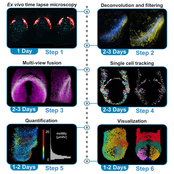
An overview of the below procedures, including the inputs and outputs of each step, is detailed in Figure 1. For a description of software packages and how they are used in this protocol, see Table 1.

Figure 1.

Overview of comprehensive workflow, partitioned by step

The step-by-step method details are broken down into discrete functions for each step. For quick reference, each segment of the protocol (5 across in the workflow, to be read left-to-right then top-to-bottom) points to numbered sub-steps (bold numbers following ‘#’) within the protocol text.

Table 1.

Software packages used in this protocol

Step(s)	Name	Description
1: #10–19	Zeiss ZEN	Proprietary Windows software included with Zeiss Lightsheet Z.1 and 7 microscopes – necessary for setup and acquisition on these instruments. For non-Zeiss imaging, refer to the software included with your microscope.
1: #14, #24–25	ZLAPS (ZEN lightsheet adaptive positioning system)	Open-source IT3 and ImageJ scripted utility (Windows) that interfaces with ZEN to provide adaptive time-lapse acquisitions. Such features may be included in future versions of ZEN or your microscope’s software, obviating this package.
2–6: #28–71	(k)ubuntu 18.04 to 24.04	Open-source Linux operating system for PC x86–64 hardware that we use for our computational workflow. User can adapt virtually all software below for Windows, although pre-built F-TGMM is only provided for Linux (user would need to download F-TGMM sources as well as nVidia CUDA toolkit and compile for Windows if desired).
2: #28–71	Fiji6 “Fiji is just ImageJ”	Open-source multi-platform Java-based application evolved from the original NIH ImageJ, with many plugins and tools included. Needed for virtually all computation steps of this workflow.
2: #28–30; 3: #44, #47; 4: #53	LSFM Processing Scripts1	Collection of macros in Fiji for automating deconvolution, filtering, and format interconversion. Additionally contains Perl and Python scripts to augment BigStitcher and TGMM integration.
2: #28–29	PSF Generator & Parallel Spectral Deconvolution	Fiji plugins that are needed for single-view deconvolution performed by LSFM Processing Scripts.
3: #31–47	BigStitcher1,7	Fiji plugin for registering (aligning) all image stacks together in 4d, and fusing them into volumes (free from motion artifact, drift, and jitter) for each time point and channel. We recommend using our multiview-reconstruction.jar (see key resources table for link to github repository) containing performance enhancements, additional user options, and Lightweight Content Based Fusion.
3–4: #47–55	KLB Fiji integration1,2 & KLB library2	System library, Python package, and Fiji utility for working with klb file format. klb is not absolutely necessary although it is highly recommended for fused datasets as the preferred format for (F-)TGMM input images.
4: #50–55	F-TGMM v2.51	Application in C++ and nVidia CUDA, compatible only with nVidia (GP)GPUs, for segmentation and tracking of fused 4d datasets (klb or tif formatted). Pre-built only for Linux, though can be built for Windows also.
3: #49; 4: #50–57; 5: #59–61	TrackingFiles	Collection of scripts, lookup tables, and configuration files for use with F-TGMM, SVF, and MaMuT.
5: #59–64	SVF1,2	Python application for statistically resolving TGMM tracking solutions into vector-like morphogenetic maps. Improves spatial accuracy and reconstructs continuous cell tracks across the full duration of the dataset. Affords backward and forward propagation of cell or tissue labels (identities) that are annotated by the user.
4: #58; 5: #64; 6: #69–70	MaMuT1,8	Fiji plugin for visualizing tracking solutions, either directly from TGMM (raw) or outputted by SVF. We recommend using our MaMuT.jar (see key resources table for link to github repository) containing additional user options and 3d viewer.
5: #55–56	MaMuT script library1	Perl scripts for manipulating MaMuT datasets via filtering, coloring, annotating, subsetting, merging, and exporting track data to visualize or quantify cell behaviors.
2–6: #28–71	LSFMProcessing-Kubuntu	USB Bootable custom live Linux distribution (Kubuntu 24.04 base) containing proprietary nVidia driers (version 550), and all software above other than ZEN and ZLAPS (see key resources table for link to GitLab repository for instructions to download and use).

Ex vivo time-lapse microscopy

Timing: 9–24 h (Note: 8–12 h user time)

Here, embryos will be harvested from pregnant dams, dissected, mounted, and subjected to multiview light sheet imaging. Prior to starting, ensure that all steps above in “prepare materials for embryo culture and imaging” have been followed, and that all necessary reagents and equipment (listed in key resources table) are available.

Optional: If using our example raw dataset to rehearse all computational steps, download all .czi.bz2 files (ignore .klb files) from our repository at Data Dryad (https://datadryad.org/stash/dataset/doi:10.5061/dryad.nk98sf823). Ensure adequate disk space (60GB) is available, and run (in Kubuntu’s Dolphin, press F4 to toggle console below folder navigation) the following command in the folder to decompress the .czi files: bunzip2 ∗.bz2. Note bunzip is single-threaded and slow. Skip to #28 below and perform processing steps on these files.

• 1.
  Prepare embryo culture and mounting reagents:

  • a.
    Melt 2–3 tubes of embryo mounting medium per dam using digital dry bath at 75°C, then transfer the tubes to a benchtop incubator at 34.5°C when completely liquid.
  • b.
    Pre-warm embryo dissection medium, embryo culture medium, PBS, and DMEM/F-12°C to 37°C.
• 2.
  When embryo mounting medium has equilibrated to incubator temperature (∼10 min), prepare and store capillaries (small/black capillaries for E6.5-E7.0, large/green capillaries for E7.5, jumbo/blue capillaries for E9.0+):

  • a.
    Use a P200 pipette to fill a glass capillary with mounting medium.
  • b.
    Once filled, orientate capillary vertically and allow medium to start to drip out of one end. As it drips down, insert plunger into that end to make a good seal with the medium (no air bubbles at the piston/gel interface).
  • c.
    Store the capillary/piston setup horizontally in benchtop incubator at 34.5°C to maintain its liquid state.
  • d.
    Repeat the above steps until 4–8 capillaries per dam are prepared and awaiting embedding.
• 3.Per dam, add 6 mL dissection medium each to two 6 cm round petri dishes; also, add 1.5 mL embryo culture medium to the center well of two IVF dishes (one for initial dissection, one for desired/chosen embryos). Temporarily store these dishes in a tissue culture incubator.
• 4.Per dam, add 12 mL PBS to a 10 cm petri dish, and add 12 mL DMEM/F-12 to another 10 cm petri dish. Place these dishes on a 37°C warm block to maintain body temperature.
• 5.
  Following established institutional protocol, deeply anesthetize and euthanize pregnant dam(s) on desired day of pregnancy.

  • a.
    Collect uterus into the 10 cm petri dish containing PBS, and swirl gently for ∼30 s to remove gross blood.
  • b.
    Transfer the uterus to the 10 cm petri dish containing DMEM/F-12 at 37°C and bring to the dissection stereomicroscope.
  • c.
    Clean the now-used warm block with 70% ethanol and return it to the 37°C digital dry bath to re-warm.
• 6.
  Following common^14,15 or user-preferred procedures, remove gestational sacs intact from uterus.

  • a.
    Transfer sacs carefully using dissection forceps (or perforated embryo spoon/ladle) into 6 cm dishes containing dissection medium.
  • b.
    Split each litter into two 6 cm dishes.

CRITICAL: Maintain 37°C as closely as possible during dissection (i.e. using temperature-controllable warming plates, working quickly).

• 7.Following common^14,15 or user-preferred procedures, microdissect embryos and remove Reichert’s membrane in each 6 cm dish.
• 8.Using a P200 pipette with low-retention wide-orifice tips, transfer each dissected embryo into the center well of the IVF dish and maintain 37°C (i.e., on temperature-controllable warming plate).
• 9.Screen embryos with a fluorescence microscope if desired, and transfer selected embryos to a fresh center well dish with embryo culture medium.

Optional: If desired, intermediate-term embryo culture can be initiated at this point by transferring embryos to the outer “moat” portion of the IVF dish containing ∼2 mL embryo culture medium in at incubator at 37°C and 5% CO₂. We recommend using an orbital shaker platform at 50–70 rpm such that embryos go around the moat like a lazy river. Culture medium should be changed every day; for this, embryos can be picked up or transferred using a 25 mL serological pipette.

Pause point: (5 min): After confirming embryos are viable for imaging and are safely stored at 37°C and 5% CO₂, we turn our attention to the microscope setup and the imaging/incubation chamber. The below steps are somewhat specific to our Zeiss Z.1 Lightsheet microscope; however, they can be easily adapted to user equipment.

• 10.
  Follow a pre-imaging checklist at the microscope:

  • a.
    Confirm thermoelectric cooler/incubation instrument has sufficient coolant. Confirm cameras (if cooled) have sufficient coolant (Figure 2Aa).
  • b.
    Ensure that correct objectives are installed (Figure 2Ab) in the microscope (we use a 20× water immersion with correction for detection), including settings on any correction collar(s) (we use RI = 1.345 for embryo culture medium). Configure software (i.e., ZEN) according to microscope configuration.
  • c.
    Install incubation sample chamber in microscope (Figure 2Ac). Ensure that top rim and lower rails are dry before installing, though other parts may remain damp from cleansing.
  • d.
    Set up tubing (Figure 2Ad), ignoring the 20 mL syringe and pump if supplemental ddH₂O is not required (see below).
• 11.
  Setup syringe with embyro culture medium:

  • a.
    Remove the plunger (stopcock closed to incubation chamber) from the 60 mL syringe, then close stopcock to the 60 mL syringe and fill with embryo culture medium.
  • b.
    After checking tubing, close the stopcock to the 20 mL syringe and slowly depress plunger of 60 mL syringe to fill the incubation chamber.
  • c.
    Close stopcock to chamber.
• 12.Use ZEN software to begin incubation at 37°C and 5% CO₂ (Figure 2Ba). Ensure that the temperature is rising and that CO₂ control is starting normally.
• 13.Use ZEN software to set up excitation and emission channels as suited for the experiment (Figure 2Bb-c).
• 14.
  If using ZLAPS, start ZLAPS (Figure 2Bd).

  • a.
    Follow instructions for configuration prior to imaging (“Usage” in https://github.com/mhdominguez/ZLAPS).
  • b.
    In the ZEN Experiment Manager tab, check “Z-Stack” and “Multiview Acquisition” and uncheck “Time Series” (Figure 2Be).

Optional: If not using ZLAPS, check “Z-Stack” and “Time Series” and “Multiview Acquisition” if desired (Figure 2Bf).

Optional: Depending on the laboratory setup and the user’s confidence in securing viable embryos for imaging, steps 10–14 above can be performed prior to embryo harvest (step 5) to decrease the time embryos are resting at 37°C and 5% CO₂ prior to imaging.

Pause point: (5 min): After confirming that the microscope is ready for imaging, we return to mounting the embryos and bringing them for auditioning on the LSFM. The below steps pertain to mounting embryos for imaging in a Zeiss Z.1 microscope; however, they can be adapted to other instrumentation.

• 15.Discard the lid from a fresh 50 mL conical vial, then tape the vial horizontally to the flat surface of the 37°C warm block, maintaining ample space on the block abutting its open top to rest capillary and piston rods (Figure 2C).
• 16.
  Remove one capillary/piston setup at a time from benchtop incubator, and keeping as sterile as possible, cool at room temperature (15°C–25°C) until the mounting medium is starting to gel (on pushing some medium out with piston, it is just barely able to maintain the cylindrical shape of the capillary). Immediately proceed to mounting an embryo with this capillary (Video S1):

  • a.
    Push down piston rod at least 25%–33% of the overall capillary length to visualize gel, then use dissecting forceps to cut gel off sharply to remove this lower portion.
  • b.
    Place the lower end of capillary (opposite the piston) into the dish containing embryos, holding it with the non-dominant hand. Use the dominant hand to push piston to extrude ∼1–2 mm of gel, then pick up dissecting forceps with dominant hand.
  • c.
    While holding capillary with non-dominant hand, use dominant hand with dissecting forceps to lightly grab the ectoplacental cone from one embryo, pushing and shoving it gently into the extruded gel from the capillary (Figure 2D).
  • d.
    Once the embryo is immobilized by adequate embedding of the ectoplacental cone into the gel, use the dominant hand (first return forceps to tabletop) to retract piston and gel column containing mounted embryo (with excess culture medium) back into the capillary. Park embryo about 4–5 mm above the lower open end of the capillary.
  • e.
    Allow capillary with mounted embryo to cool to room temperature (15°C–25°C) for 1–2 min, then place capillaries inside open-top horizontally-oriented conical vial at 37°C prepared above.

Figure 2.

Ex vivo time lapse microscopy

(A) Microscope Preparation (Steps 10a–d): Setup and checks before imaging including confirmation of coolant levels and objective installation, and preparation of the incubation sample chamber and tubing.

(B) Incubation and Software Configuration (Steps 11–14): Initial setup of the incubation environment using ZEN software, configuring the excitation and emission channels, and additional setup for ZLAPS, if used.

(C) Temperature Maintenance after Mounting (Step 15): Conical vial is taped to warm block to use as storage/transfer device for embryo-loaded capillaries.

(D) Embryo Mounting (Step 16): Detailed procedure for mounting embryos for imaging, including adjusting piston rod and embryo placement into capillary.

(E) Embryo Positioning for Imaging (Step 19): Placement of embryo-containing capillary into the microscope stage and initial positioning for imaging.

(F) Capillary Securement in Microscope (Step 22): Securing capillary on the microscope stage for stable time lapse imaging. Use of parafilm to minimize downward movement of the piston rod during a long experiment.

(G) Z-stack and Multiview setup in ZEN (Step 24): Configuration of Multiview settings, initiation of time lapse imaging, and environmental conditions maintenance.

(H) Tank setup (Step 25): Checks on medium level in the tank, presence of white tank cover to prevent dehydration, and connection of tubing including CO₂.

Video S1. Embryo mounting for multiview live imaging (Step 16)

Embryo must be trimmed for unobstructed illumination and observation from multiple angles with respect to region of interest. Ectoplacental cone is pushed into a column of partially-gelled agarose/gelatin mix for 360° free imaging of embryonic region.

Troubleshooting 1: Mounting embryos requires patience, practice, and optimization of the gelling conditions may be needed for best results.

• 17.Repeat previous step for each embryo. When all embryos are mounted, carefully move the 37°C warm block with conical vial and capillaries to the microscope room.
• 18.Confirm microscope setup is appropriate, with no leaks in incubation chamber or tubing, no leaks in peltier/TEC coolant connections, and that incubation is running at 37°C and 5% CO₂.

Optional: If desired, verify the culture medium pH using a sterile transfer pipette/dropper and test strips (i.e. Chemstrip 10).

• 19.
  Load the first embryo-containing capillary into the capillary holder (Figure 2E), then:

  • a.
    Seat the capillary holder onto the microscope stage.
  • b.
    Using ZEN Specimen Navigator to position the stage, move capillary into the working position just above the objectives’ field of view.
  • c.
    Under camera visualization, slowly push piston rod to lower embryo freely into surrounding culture medium.

Note: Do not extend the agarose column into the immersion medium more than is necessary for imaging the critical aspects of the embryo.

• 20.
  Focusing on areas of the specimen that are NOT the subject of the live imaging experiment, align the light sheets in the detection plane.

  • a.
    Ensure pivot scanner (if equipped) is enabled, and that Online Dual Side Fusion is enabled (depending on embryo size, photon budget, and intended multiview setup).
  • b.
    If imaging more than one channel, ensure that alignment of light sheets is correct in all channels (all channels should align simultaneously), and if not, consult technical support.
• 21.
  Quickly obtain auditioning views of the specimen, then change capillaries to audition each embryo that has been mounted:

  • a.
    Upwardly retract piston rod under camera visualization to park embryo a few mm above bottom of capillary.
  • b.
    Raise the stage to its loading position to unmount.
• 22.Select the desired embryo for time lapse imaging, and load its capillary into the microscope again as above.

Note: If using Z.1 and similar top-load microscopes, after positioning the embryo into the objectives’ field of view, carefully open microscope loading platform and use parafilm to tightly wrap the piston rod to the thumbscrew (Figure 2F). Wedging parafilm between the thumbscrew and piston rod is also helpful to prevent unintended downward movement of the piston during imaging (Figure 2F).

• 23.Verify light sheet alignment. Configure objective zoom, accounting for growth of the specimen during the experiment (though this can be adjusted later as needed).

CRITICAL: Adequate segmentation in computational steps requires adherence to both Nyquist and segmentation scale principles. The distance separating the borders of the closest adjacent nuclei should be at least twice (preferably several fold greater to account for aberration, noise, and other artifact) the pixel scale factor at acquisition. At E6.5, the most densely packed nuclei have boundaries that are offset by as little as 600–800 nm; therefore, we recommend 0.3 μm/pixel (or smaller) imaging resolution.

• 24.If using ZLAPS, follow configuration steps and start imaging. Otherwise, configure Multiview-Setup (Figure 2G) and acquire a first time point. Place tank cover to prevent dehydration.
• 25.
  Follow an imaging checklist to systematically ensure smooth operation. An example of such a standard operating checklist we have employed before/during a live LSFM experiment:

  • a.
    ✓ incubation is running at 37°C and 5% CO₂ (Figure 2Ba).
  • b.
    ✓ medium level in sample tank is good, with no apparent leaks (Figure 2H).
  • c.
    If desired, verify culture medium pH and/or density/specific gravity using a sterile transfer pipette/dropper and test strips (remove tank cover).
  • d.
    ✓ stopcock in correct position.
  • e.
    ✓ if applicable, supplemental ddH₂O setup is adequate with correct levels (Figure 2Ad).
  • f.
    ✓ if applicable, supplemental ddH₂O is primed and running.
  • g.
    ✓ tank cover in place to prevent dehydration (Figure 2H).
  • h.
    ✓ lightsheets in good alignment.
  • i.
    ✓ objective zoom is correct (if mag changer available).
  • j.
    ✓ laser power setting is appropriate for the stage and experimental plan (Figure 2Bb).
  • k.
    ✓ embryo position and view angles are good, with region of interest near the center of each Z-stack.
  • l.
    ✓ multiview set-ups established correctly and in proper order.
  • m.
    ✓ time lapse imaging set-up at correct intervals (we recommend 6 min for whole cell tracking at E6-E7) with sufficient time points requested.
  • n.
    ✓ sufficient hard drive space on destination.
  • o.
    GO first time point! Ensure first time point captures correctly.
  • p.
    ✓ second time point appears to be capturing correctly.
  • q.
    ✓ ZLAPS appears to be working.
  • r.
    ✓ signs are posted to indicate that a live experiment is taking place.

    CRITICAL: If long term (6+ h) imaging will be undertaken, we recommend checking that the medium level in the sample chamber remains adequate. If evaporation is occurring, user can verify medium pH and density/specific gravity as described in the above checklist. Light sheets may need alignment adjustment every few hours depending on the instrument.

    Optional: If pH is not in the desired range (usually 7.4 to 7.5), adjust CO₂ concentration accordingly.

    Optional: If sample chamber medium level is declining, and density or specific gravity measurements indicate that evaporation is taking place, set up supplemental ddH₂O syringe and pump:

  • s.
    Close stopcock to the unattached sideport if it is not already in this position.
  • t.
    Fill a 20 mL syringe with sterile deionized water (i.e., cell culture grade), attach it to Luer tubing and prime the tubing by depressing the plunger.
  • u.
    Connect the other end of the tubing to the stopcock. Close the stopcock to the sample chamber.
  • v.
    Slowly depress the plunger of the 20 mL syringe in order to evacuate any air bubbles into the inverted culture medium syringe, and away from the sample chamber.
  • w.
    Close the plunger to the 60 mL syringe and begin pump operation. We recommend starting at ∼5 μL/min flow and adjusting as needed to maintain a good level of medium in the sample chamber.
• 26.Each time the user walks away from the live imaging setup (regardless of the time), we recommend following a similar checklist to maximize endurance of the experiment.

CRITICAL: The stage at the onset as well as total duration of the imaging acquisitions should depend on the biological process under study. Our example dataset is approximately 3 h long; however, for study of migration and morphogenesis of early heart formation in the mouse, an adequate duration is 9–24 h depending on experimental design. The embryos should be harvested at a stage (at least several hours to account for variability) prior to the biological events being captured. Embryo culture medium recipe should be modified for optimal development at that stage.^11,12,15

• 27.
  When the experiment is finished, take care to follow the reverse of the setup steps. In addition:

  • a.
    Consider rechecking pH and density or specific gravity, and note these values for titration of CO₂ and supplemental ddH₂O flow rate in future live imaging runs.
  • b.
    Ensure sample chamber and all fittings that contact the culture medium are adequately sanitized with 10% bleach and/or 70% ethanol. We recommend periodic disassembly of the sample chamber for scrubbing, immersion, and/or sonication of its components (where appropriate).

Pause point: After data is collected, processing can commence at any time. Remember to backup each raw dataset after it is collected. The remaining steps in this protocol can be followed straightforwardly, or can be easily adapted to images acquired on microscopy equipment other than that described above. Since data processing can proceed at user’s pace, there are no further Pause points in the protocol.

CRITICAL: In planning image acquisitions (#22–25 above), users must consider the overall goals of their experiments, size and accessibility of region(s) of interest (ROI) within the specimen, the microscope they are using, their photon budget, as well as other factors (Figure 3A). Time lapse imaging usually requires trade-offs between temporal and spatial resolution, as finer time granularity may limit the available time to acquire images/views for each frame and vice-versa.

Note: Our own experience and empirical testing has informed our typical acquisition of two channels (488 nm, 561 nm) with 2–3 views offset at 72°–110° in the y-axis. This multiview setup is compatible with 6-min interval imaging of early mouse embryos on a Zeiss Z.1. We initially process our raw images with single-view deconvolution and enable additional de-blurring, since the alternative approach – multiview deconvolution – is inefficient when fusing fewer than 4 views.¹⁶ Users should critically examine their own experimental goals and equipment before deciding on an imaging plan. Iterative planning through experiential learning during imaging and processing steps is beneficial for optimizing an experiment’s photon budget and recovery of high signal-to-noise data, together with downstream user and CPU time.

Figure 3.

Deconvolution, filtering, and multiview registration

(A) Pre-Processing Workflow Overview (Steps before 28): Visual representation of the recommended workflow for image acquisition and considerations, including setup and planning for multiview imaging.

(B) Initial Image Deconvolution and Filtering (Steps 28–30): Setup, parameter adjustment, and execution of LSFMProcessing macros in Fiji for deconvolution.

(C) Data Import and Pre-processing for BigStitcher (Step 32): Steps for importing and re-saving data in the BigStitcher-friendly h5/xml format.

(D) Interest Points Detection (Step 33): Process of detecting interest points within the datasets for image registration, with adjustment of detection parameters shown.

(E) Initial 3D Pre-Registration Using Interest Points (Step 34): Pre-registration in 3D using interest points detected earlier, detailing settings adjustments for optimal registration.

(F) Fine 3D Registration (Step 35): Detailed view of the fine registration process in 3D, with specific algorithm adjustments.

(G) Initial 4D Pre-Registration (Step 36): Setup and pre-registration across time points in 4D, using rigid transformation.

(H) 4D Series Undrift Using Center of Mass (Step 37): Procedure for correcting positional drift over time using the center of mass algorithm, selecting a mid-sequence reference time point.

(I) Repeating 4D Pre-Registration (Step 38): Repeat of the initial 4D pre-registration to refine alignment after undrift, emphasizing increased time point matching range.

(J) Fine 4D Registration (Step 39): Fine registration in 4D, focusing on optimizing view and time point overlap, with rigid or affine transformations.

(K) Unconstrained 4D Registration for Improved Tracking (Step 40): Advanced registration step to enhance tracking accuracy by allowing more flexible correspondence between time points (without view constraints).

(L) Re-Registration in 3D Unconstrained in Time (Step 41): Re-registration in 3D without time constraints, aimed at improving the fit of multiview datasets across different registration stages.

(M) Final Fine 4D Registration (Step 42): Completion of the registration process with fine adjustments in 4D, maximizing alignment and transformation accuracy over extended time points and views.

Deconvolution and filtering

Timing: 2 days (30 min user time)

In this step, our workflow employs single-view CPU-based deconvolution and additional de-blurring, which are followed by registration in the next step. In other words, raw images from each view will be processed prior to registering and fusing those images into a solid in toto volume.

Optional: For 4 views, if desired, skip to #32 and use Multiview Deconvolution in #46. Users should consult our recommended workflow (Figure 3A) prior to advancing to this step, especially if acquiring more than 3 views (i.e. SiMView, MuVi SPIM LS) or if using different instrumentation than we describe here.

• 28.Open Fiji, install LSFMProcessing macros as instructed (https://github.com/mhdominguez/LSFMProcessing), and adjust deconvolution settings (Figure 3Ba-b, Plugins → Macros → 0. Change LSFM processing settings...).

Note: For 64 GB RAM/heap and 4 megapixel image slices, we recommend setting maximum block depth at maximum 320 slices; while for 120 GB RAM/heap we recommend maximum 480 slice blocks. Within the same settings window, adjust filtering settings as desired, including the application of additional deblurring, range compression to 8-bit, and/or stack depth uniformity.

• 29.Run deconvolution on the raw 4D dataset. (Figure 3Bc, Plugins → Macros → 1. Deconvolve Z.1 time series (folder in batch)…). Follow instructions to select input and output folders.
• 30.If desired, run post-deconvolution filtering (2. Filter and unify z-depth of LSFM .tif files (best for time series; folder in batch)…).

Note: As shown above in #28, user settings will affect which methods are used in this step. The output folder of deconvolution is the input folder in this step. This step’s output will be written to a new “Filtered” sub-folder.

CRITICAL: Ensure ample disk space is available on destination drive at each step. Expect deconvolved and filtered image sets each to consume similar space as the original raw images.

Multi-view fusion

Timing: 2 days (2–8 h user time)

This step imports image data into BigStitcher, a Fiji plugin for registering (aligning) all image stacks together in 4d, and fusing them into a single volume (free from motion artifact, drift, and jitter) for each time point and channel.

Optional: Datasets with 4 or more views (i.e. those collected on SiMView, MuVi SPIM LS, and similar microscopes) can take advantage of multiview deconvolution in BigStitcher rather than single view deconvolution prior to BigStitcher import (Figure 3A). If this is the case, user can import raw acquired image data and re-save as h5/xml (i.e. SiMView) or can use images already collected in h5/xml format (i.e. MuVi SPIM) and then proceed here for BigStitcher registration.

• 31.In Fiji, run BigStitcher (Plugins → BigStitcher → BigStitcher).
• 32.
  Import outside data and re-save in BigStitcher/BDV format (Figure 3C):

  • a.
    Click Define a new dataset.
  • b.
    Using Automatic Loader, proceed (“OK”) to specify the input files. If user is importing raw unprocessed images with intention of fusing with multiview deconvolution, another import method (i.e., Zeiss Lightsheet) may be appropriate.
  • c.
    Excluding files below 1,000 kB (to exclude log files and PSFs), choose the input directory, which should be the Filtered folder created in #30 above, or the deconvolved output folder (#29 above) if skipping step #30.
  • d.
    Choose filename patterns to identify different channels, time points, and views (T = time point, C = channel, A = angle, as in Figure 3Cd).
  • e.
    Confirm that angle information is correctly parsed by the BigStitcher importer (Figure 3Ce).
  • f.
    Choose re-save h5/xml output format, and select the dataset export path (Figure 3Cf).

    CRITICAL: Ensure ample disk space is available on destination drive.

  • g.
    Confirm h5/xml settings (Figure 3Cg). We recommend splitting datasets by time point and view setup (i.e., combination of channel and angle).
• 33.
  Detect interest points for registration (Figure 3D):

  • a.
    When import and re-save is complete, BigStitcher will open the dataset (Figure 3Da).
  • b.
    In Multiview Explorer, sort/rank images by Channel, then select all images belonging to an appropriate channel (i.e., nuclei, punctae, etc.). Right-click and select Detect interest points from the Multiview Explorer context menu (Figure 3Db).
  • c.
    If using an 8-bit dataset, choose Set minimal and maximal intensity; otherwise, proceed (“OK”) with Difference-of-Gaussian detection (Figure 3Dc).
  • d.
    Select 2× in Downsample XY (Figure 3Dd). If using 8-bit, choose 0 and 255 as the minimum and maximal intensities.

    Note: Different Downsample options will affect accuracy and computation time, and can be tested empirically for datasets of different size and resolution.

  • e.
    When prompted, select the time point and view you would like to visualize for detection of interest points (Figure 3De).

    Note: Typically Timepoint 0, Viewsetup 0 can work. However, if the signal intensity/quality declines through the dataset, we recommend choosing an intermediate time point.

  • f.
    Moving/resizing the ROI box to the sample data, adjust Sigma (radius of the Gaussian) and Threshold (intensity of the Gaussian) to maximize correct detections while minimizing noisy/incorrect detections (i.e., those noted in the void away from the sample).

    Note: For our acquisitions, we use a Sigma ∼5 pixels, and for our 8-bit dataset we adjust the Threshold slider to near 0.002 (Figure 3Df).

    Troubleshooting 2: Careful selection of interest point detection parameters can markedly improve registration results. User must interactively move within the z-stack to ascertain correct sigma and threshold settings for minimal background detections.
  • g.
    Save the dataset in Multiview Explorer. Frequent saving between subsequent steps is recommended.
• 34.
  Pre-register in 3d (Figure 3E):

  • a.
    Select all images from the channel where interest points were detected. Right click in Multiview Explorer and select Register using Interest Points… (Figure 3Eb).
  • b.
    Comparing all views and all interest points, use the Fast descriptor-based (translation invariant) algorithm to Register timepoints individually, using the interest points found above (Figure 3Eb).

Note: On our datasets, we fit with Translation transformations, turn off Regularize model, and reduce Significance required for a descriptor match as well as Inlier factor to improve correspondences (interest points that match between images/views) in this initial pre-registration step (Figure 3Ec). Decreasing Redundancy for descriptor matching usually improves the speed of the registration.

CRITICAL: User should become familiar with the BigStitcher registration workflow. Each time Register using Interest Points… is used, a new transformation matrix is concatenated to the stack of registrations (matrices) for any image (each image/view is displayed in a distinct row in Multiview Explorer), incrementing the # Registrations for that line. At the time of image fusion, each view’s matrix stack is collapsed into a single transform matrix to bring that view into alignment with the others in the fused volume. Be familiar with the Transformation model options that are available: Translation (movement in X, Y, and/or Z), Rigid (Translation plus rotation in X, Y, and/or Z), and Affine (Rigid plus scale and shear). Non-rigid transformations – those that go beyond Affine fitting (i.e. mesh/cage warp, etc.) – are not accepted during registration but can be applied during Image Fusion, leveraging corresponding interest points in the registered images/views.

CRITICAL: To undo any registration step, ensure all images/views that were registered are selected in Multiview Explorer(they normally remain selected when methods are called), then right click and select Remove Transformation→ Latest/Newest Transformation from the context menu. Do this whenever an undesired transformation occurs (i.e. view alignment worsens, not improves) either through Register using Interest Points… or Apply Transformation(s).

• 35.
  Finely register in 3d (Figure 3F):

  • a.
    Select images from channel where interest points were detected. Right click in Multiview Explorer and select Register using Interest Points….
  • b.
    Comparing only overlapping views but all interest points, use the Assign closest-points with ICP (no invariance)algorithm to Register timepoints individually, using the interest points found above (Figure 3Fa).

Note: We typically run ICP with Rigid or preferably Affine transformation models, enabling Regularize model, and disabling Use RANSAC (Figure 3Fb). We typically do not change the regularization Model or Lambda value from its default setting (Figure 3Fc).

• 36.
  Pre-register in 4d (Figure 3G):

  • a.
    Select images from channel where interest points were detected. Right click in Multiview Explorer and select Register using Interest Points….
  • b.
    Comparing all views and all interest points, use the Fast descriptor-based (translation invariant) algorithm to register over time using All-to-all timepoints matching with range, with the interest points found above (Figure 3Ga).

Note: Because this is a pre-registration step, we decrease the sliding window Range for all-to-all timepoint matching to 3, and enable Consider each timepoint as rigid unit. To account for temporal to shifts in specimen positioning, we use Rigid transformation model, and leave other settings similar to pre-registration in 3d above (Figure 3Gb-c).

• 37.
  Undrift series in 4d (Figure 3H):

  • a.
    Select images from channel where interest points were detected. Right click in Multiview Explorer and select Register using Interest Points….
  • b.
    Comparing all views and all interest points, use the Center of mass algorithm to register over time using Match against one reference timepoint (no global optimization), using the interest points found above (Figure 3Ha).
  • c.
    Choose a high-quality single time point in the middle of the series to use as Reference timepoint, and enable Consider each timepoint as rigid unit.
• 38.Repeat pre-register in 4d (Figure 3I) now that positional drift is corrected. Follow steps in #36 above. However, increase the Range for all-to-all timepoint matching in this step to at least 5 for improved precision and smoothness of temporal registration.

Optional: The above two steps (#37 and #38) can be omitted if positional drift is minimal in your dataset, but we recommend checking for this (by fusing example time points from beginning to end and viewing as 4d hyperstack) after step #36 if you intend to skip #37 and #38. All-to-all timepoints matching with range is excellent for finely registering in 3d and 4d, but slow drift in the specimen center can accumulate over longer time durations, which unnecessarily increases the final fused volume and adds artifactual movement in cell tracking.

Troubleshooting 3: Temporal or spatial gaps in registration are common in large datasets, and require additional registration steps with alternate settings.

• 39.
  Finely register in 4d (Figure 3J):

  • a.
    Select images from the channel where interest points were detected. Right click in Multiview Explorer and select Register using Interest Points….
  • b.
    Comparing only overlapping views but all interest points, use the Assign closest-points with ICP (no invariance)algorithm using All-to-all timepoints matching with range, with the interest points found above (Figure 3Ja).
  • c.
    Set Range for all-to-all timepoint matching to 3, and enable Consider each timepoint as rigid unit. Similar to step #35, use Rigid or Affine transformation models, enabling Regularize model, and disable Use RANSAC (Figure 3Jb).
• 40.
  Finely register in 4d while each time point’s images/views are unconstrained (Figure 3K). This step improves tracking accuracy through better registration across time while not holding images/views rigidly together at each time point.

  • a.
    Select images from channel where interest points were detected. Right click in Multiview Explorer and select Register using Interest Points….
  • b.
    Comparing only overlapping views but all interest points, use the Assign closest-points with ICP (no invariance)algorithm using All-to-all timepoints matching with range, with the interest points found above (Figure 3Ka).
  • c.
    Set Range for all-to-all timepoint matching to 5, and disable Consider each timepoint as rigid unit. Use Affine transformation, enable Regularize model, and disable Use RANSAC (Figure 3Kb).

Note: Increase Maximal distance for correspondance (px) as needed to align images/views that are not in close proximity before this step.

• 41.Finely re-register in 3d, now unconstrained in time. This step is paired with the above and below steps to improve overall 4d fitting of multiview datasets. Follow a similar procedure as that in step #35 above (Figure 3L).
• 42.Complete final fine registration in 4d, using a similar procedure to step #39, except increase Range for all-to-all timepoint matching to at least 5, and use Affine transformation model (Figure 3M).

Video S2. Time-lapse sequences of projection images and dataset renderings (Steps 49 and 70–71)

Example expected results for presentation, including multichannel maximal projections, SVF/MaMuT reconstructions, and single-channel anaglyphs (for viewing with red/blue 3d glasses).

Troubleshooting 4: ICP (iterative closest point) registrations have some pitfalls with model overfitting, and may need parameter tweaking to account for large temporal or spatial movements between time points. Generally, we recommend Regularize model, especially for Affine transformations.

• 43.
  When the single channel is satisfactorily registered in 4d, apply rigid rotation transformations to align the specimen with the XYZ coordinate system for fusion.

  • a.
    To examine specimen’s current orientation, use Multiview Explorer to select all images/views from at least one time point in the now-registered channel, right click and choose Image fusion… (Figure 4Aa).
  • b.
    In the Image Fusion dialog, select Display using ImageJ with Downsampling at 4 or greater, 16-bit Pixel type, Non-Rigid disabled, Content based fusion disabled, and Precompute images (Figure 4Ab).
  • c.
    The fused image volume will appear as a new Fiji image. From the menu, use Image → Stacks → Z Project… to create a maximum projection in the YZ plane (Figure 4Ac).

    Optional: We recommend creating and using keyboard shortcuts for Z Project… and other frequently used functions (Plugins → Shortcuts → Add Shortcut…).

  • d.
    Use the Angle tool to draw the rotation needed (estimate) in Z to align the specimen with the XY axis (Figure 4B). Type ‘M’ to measure this angle.
  • e.
    Return to Multiview Explorer, and select all images/views from the channel where interest points were detected to rotate the specimen:

    • i.
      Right click in and select Apply Transformation(s)…(Figure 4C).
    • ii.
      Choose Rigid for Transformation model, and select Define as Rotation around axis.
    • iii.
      Enter z-axis and the measured angle (Figure 4C).
  • f.
    Repeat fusion and maximum projection as above (#43a-c) to confirm proper alignment with the XY axis (Figure 4D).

    Note: If the specimen rotates the wrong direction, either undo the transformation or repeat rotation (#43e above) using negative of the rotation angle. Each transformation step can be undone with Remove Transformation→ Latest/Newest Transformation.

  • g.
    Use orthogonal view projections to check rotation and alignment:

    • i.
      Choose the window containing the newly aligned fused volume, and use Image → Stacks → Reslice [/]… with Rotate 90 degrees enabled and Start at: either Top or Left (Figure 4E).
    • ii.
      Create a maximum projection of the resliced image volume in either XZ or YZ planes (following #43c above) and estimate the rotations needed to align the specimen in those axes (following #43d above).
    • iii.
      Apply the rotations and recheck specimen alignment (following #43e-f above).
  • h.
    Repeat this step iteratively until the specimen is satisfactorily rotated in all axes. An alternative to this process involving fusing and angle measurements (#43a-g above), user can use BigDataViewer to apply free and interactive manual transformations (Figure 4F).
• 44.
  Copy view transformations from the registered channel (with the interest points) to all other channels (Figure 4G).

  • a.
    Save dataset in Multiview Explorer, then close.
  • b.
    Open the console/command line and navigate to dataset folder (in Kubuntu’s Dolphin, press F4 to toggle the console panel that appears below folder navigation).
  • c.
    Ensure Perl is installed (if Windows), and that dataset_folder_copy_view_transformations.pl is copied to that folder.
  • d.
    Run in terminal:

    $ perl dataset_folder_copy_view_transformations.pl.

    Note: The script will modify dataset.xml and print correlated view setups for which it updated the transformation matrix stack (Figure 4G).

  • e.
    Re-open dataset in BigStitcher. Confirm that all channels are now co-registered.
• 45.
  Setup the narrowest bounding box (Figure 4H):

  • a.
    Select all images/views in Multiview Explorer (any image selection is acceptable).
  • b.
    Right click in and select Define Bounding Box… from the context menu. Choose Define using the BigDataViewer interactively (Figure 4Hb).
  • c.
    Adjust the XYZ extremes of the bounding box, visualizing specimen and box with BigDataViewer (the bounding box interior is shaded purple).
  • d.
    Narrow the boundaries as much as possible without excluding regions of the specimen.

CRITICAL: Ensure that the entire 4d specimen (or at least the region of interest) is included in the box. Be careful to check that the entire Z (mouse wheel +/− Ctrl) and T extents of the specimen are in-bounds of the box.

• 46.
  Export in toto image volumes using lightweight content based fusion (or multiview deconvolution) (Figure 4I).

  • a.
    Select all images in Multiview Explorer (Ctrl+A) (Figure 4Ia).
  • b.
    Right click in and select Image Fusion…. Use 16-bit pixels (or 8-bit if previously range-compressed), Linear Interpolation, Cached image loading (to decrease heap memory usage). Configure Image Fusion settings:

    • i.
      If using our multiview-reconstruction.jar plugin, choose the orientation of the fusion. Current XYZ orientation will create a Z-stack in the as-seen orientation in BigDataViewer, whereas other orientation options will create side or top views.
    • ii.
      Set your desired output Anisotropy in Z (we use 4× anisotropy for all fusions).

      CRITICAL: If using Anisotropy in Z (see above), fuse with the most appropriate view/angle to maximize resolution in the axis of expected cell movement for downstream tracking.

      Optional: If stacks are Z isotropic at time of fusion, consider reslicing and rotating the stacks after fusion – to create the most desirable view for tracking – then manually downscale in Z.

    • iii.
      Disable (faster, best for testing fusions) or Enable (slower, best for final fused output) content based fusion.

      Note: We recommend lightweight content based fusion from our multiview-reconstruction.jar, using 2×downsampled weights.

    • iv.
      Save fusions for each time point and channel, in xml/hdf5 format (Figure 4Ib).

      Optional: If fusing 4 or more views, (MultiView) Deconvolution… may improve the quality of fused image volumes compared with [lightweight] content based fusion. To generate theoretical point spread function (PSF) files, run step 1 of LSFMProcessing with deconvolution actually disabled (Plugins → Macros → 0. Change LSFM processing settings…to disable deconvolution, then Plugins → Macros → 1. Deconvolve Z.1 time series (folder in batch)…). This will create _psf.tif files in the raw dataset director, for each view or channel requiring a separate PSF. Follow BigStitcher instructions to Assign…those external PSF .tif files to each view setup (channel / angle combination). With multiview deconvolution, we typically use default settings with Optimization II, and Z-anisotropy of 1 (i.e. isotropic in Z). When fusions are exported as Z isotropic, we subsequently generate front and side views with anisotropy at 4 by downscaling the Z-axis (preceded by optional reslicing if an orthogonal view is desired) using batch processing. Z isotropic output images tend to be large and extremely costly to process versus Z-anisotropic.

  • c.
    In subsequent Save as new XML Project options, enable split hdf5, with 1 time point per partition and 1 setup per partition (Figure 4Ic). Ensure ample free memory and disk space in target drive before proceeding to Image Fusion or Multiview Deconvolutions.

    Note: Newer and official versions of multiview-reconstruction.jar (does not apply to our GitHub-supplied version) may have additional options at the time of fusion. The default settings are often appropriate, but we recommend consulting the online BigStitcher documentation for assistance.

• 47.
  For downstream compatibility and improved lossless compression, use LSFMProcessing macros to convert .h5 files in the fused dataset folder(s) to klb format.

  • a.
    Open Plugins → Macros → 4. Convert fused .h5 to .klb… (Figure 4J).
  • b.
    Ensure ample free space on disk before proceeding.
  • c.
    Follow prompts to choose folder location of the h5/xml dataset.

Note: This requires a complete installation (including dependencies) of LSFMProcessing.

Optional: If using our sample fused dataset to rehearse tracking and quantification steps, download all .klb files from (ignore .czi.bz2 files) our repository at Data Dryad (https://datadryad.org/stash/dataset/doi:10.5061/dryad.nk98sf823) to a unique folder location. Proceed from #48 below. For creating the dataset.xml file, the pixel spacing in this dataset is 0.3044 microns in XY and 2.0 microns in Z.

• 48.
  Recommended: Create a BigDataViewer dataset.xml file to pair with klb files generated in the above step (Figure 5A).

  • a.
    Open the original multiview (not fused) dataset.xml in Kate or other text editor (Figure 5Aa). Search (Ctrl+F) for voxelSize and observe the X or Y pixel dimension value from the <size> tag as shown, which is populated by three space-delimited (floating point) numbers that reflect the X Y Z voxel size, usually in μm.
  • b.
    Open KLB importer via Fiji menu (Figure 5Ab): Plugins → BigDataViewer → Open KLB(or use Plugins → Macros → 5. Create .klb BigDataViewer dataset.xml file…).
  • c.
    In the middle-lower portion of the dialog (Figure 5Ac), enable Manually specify pixel spacing (μm).

    • i.
      Enter the X and Y pixel unit sizes to the right of Manually specify pixel spacing (μm).
    • ii.
      Compute and enter the Z voxel size by multiplying this X voxel dimension by the Z anisotropy factor that was chosen during fusion (#46 above).
  • d.
    At the top of the dialog (Figure 5Ac), to the far right of Template file, click … and choose the first klb image, usually named t00000_s00.klb. Set up the filename pattern for all subsequent images:

    • i.
      In the table below, modify Color channel to be file path tagged with ‘s’ (no quotes) and Time to be tagged with ‘t’.
    • ii.
      Set First for both Color channel and Time to 0, and set Stride for both to 1.
    • iii.
      Set Last for Color channel or Time to [number of channels or time points – 1], as observed in the t00??? or s0? values among klb files.
  • e.
    Click Save XML to write a new dataset_klb.xml file that can be used in BigDataViewer (or BigStitcher) with the klb files.

    Optional: After the .klb dataset is created, user may opt to archive/backup the pre-fusion multiview h5/xml dataset files (∗.h5 and [usually] dataset.xml used in steps #31–45 above) and raw (czi, tif, or h5) data (from steps #1–27 above), while deleting intermediate steps that are more facilely and algorithmically reproducible (such as deconvolved image stacks, and/or post-deconvolution filtered image stacks). After following optional step #48 above, the fused h5/xml dataset) can be considered an intermediate step and deleted or archived; if not using klb/xml, user will need to preserve the fused h5/xml dataset for downstream use in MaMuT.

• 49.
  Generate projection images and anaglyphs for visual presentation of the 4d dataset (Figures 5B and 5C).

  • a.
    Open maximum intensity projection (MIP) exporter from the Fiji menu (Figure 5Ba): Plugins → Macros → 5. Convert t0XXXX .klb/.tif files to anaglyphs or MIPs (folder in batch)….
  • b.
    Select the folder containing the klb dataset.
  • c.
    In the KLB/TIF processing settings dialog (Figure 5Bc), choose the desired views and projections.

    Note:Custom partial z-MIP settings… can be used to generate cutaway views of the specified slices; however, user must know the slice #’s before opening the MIP exporter. We recommend previewing a few .klb images throughout the time series to determine if cutaway views may be helpful to show morphogenetic phenomena that may address goals of the study. These previews will allow the user to find the slice #’s that should be entered in Custom partial MIP settings….

  • d.
    Confirm that a new folder, “MIPs”, was created in the klb dataset directory, and that tif files have been generated for each desired view or projection (Figure 5Bd).

    CRITICAL: Ensure ample disk space is available.

  • e.
    Open the MIP to avi converter (Figure 5Ca) from the Fiji menu: Plugins → Macros → 6. Process t0XXXX MIPs (folder in batch) to AVIs…. Select the MIPs folder created above (Figure 5Cb), then choose the desired MIPs, channels, time points, and other settings (Figure 5Cc).
  • f.
    For each channel merged in the final .avi files, a lookup table (LUT) is needed for pseudocoloring (Figure 5Cd-e).

    Note: A one-channel LUT (Dominguez-1col-red.lut) and a two-channel LUT set (Dominguez-2col-green.lut, Dominguez-2col-magenta.lut) can be found in ∼/Downloads/TrackingFiles/luts, though user may wish to use different colors or spectra depending on the number of channels and the presentation aims.

  • g.
    Confirm creation of the .avi files in the AVIs subfolder within the MIPs folder, with the movies selected above (Video S2).

Figure 4.

Multiview fusion

(A) Initial Specimen Fusion and Orientation (Steps 43a–c): Examination of specimen orientation.

(B) Specimen Rotation for Axis Alignment (Step 43d): Using the Angle tool to measure and estimate necessary rotation in Z to align the specimen with the X/Y axes.

(C) Application of Rotation Transformations (Step 43e): Applying measured rotation angles to the specimen for correct alignment in axes.

(D) Verification of Specimen Alignment (Step 43f): Repeating fusion and projection to verify correct alignment after applying rotation.

(E) Reslicing and Final Axis Alignment (Step 43g): Iterative reslicing and projection to align the specimen in other axes, refining rotation adjustments as necessary.

(F) Manual Transformation Adjustments (Step 43h): Utilizing BigDataViewer for manual adjustments to facilitate specimen alignment.

(G) Copying Transformations Across Channels (Step 44): Script-based automation to copy view transformations from one channel to all others, ensuring co-registration.

(H) Defining the Narrowest Bounding Box (Step 45): Interactive definition of the bounding box using BigDataViewer to ensure all specimen parts are included without excess space.

(I) Fusion Export and Setup (Step 46): Configuration of settings and execution of multiview fusion.

(J) Conversion to klb Format (Step 47): Using LSFMProcessing macros to convert fused image volumes from .h5 to .klb format, optimizing for downstream processing and storage efficiency.

Figure 5.

Projection image sequences for presentation

(A) Creating BigDataViewer dataset.xml for klb Files (Step 48): Facilitate the use of BigDataViewer with the klb dataset.

(B) Generating Projection Images (Step 49a-d): Processing of .klb files to create maximum intensity projection (MIP) images for visual analysis.

(C) Converting MIPs to AVI Format (Step 49e-g): Conversion of MIP images into video format, incorporating color adjustments and other presentation settings.

Single-cell tracking

Timing: 2–3 days (4–6 h user time)

Following export to klb format, single-cell tracking identifies each cell at each time point, then uses linear modeling and/or logical rules to link each cell with its future self in subsequent time points. Here, we will use F-TGMM to track our 9-time point example (fused from the frontal/coronal view) with anisotropy factor of 4.

Alternatives: For mouse embryo datasets, we have found excellent linkage fidelity for TGMM 2.0^2,3 and F-TGMM v2.5¹ during cell migration, though relatively poorer results with accurately linking mother and daughter cells during division.¹ Besides these, there are other tracking methods that users can substitute here.^9,17

Optional: If using our example fused .klb dataset to rehearse tracking and quantification steps, download all .klb (ignore .czi.bz2) files at our Data Dryad respository (https://datadryad.org/stash/dataset/doi:10.5061/dryad.nk98sf823) to a unique folder location. Ensure there is adequate disk space. Follow #48 above and subsequent steps. For creation of the dataset.xml file, the pixel spacing in this dataset is 0.3044 microns in XY and 2.0 microns in Z. If you wish to skip this tracking step and proceed to Tracking quantification below, navigate to the klb dataset folder in the console or in Dolphin with console panel (use F4 to toggle). At the console in this folder, run mkdir"GMEMtracking3D_$(date +%s)" to create the tracking folder. Copy TGMM_result.tar.gz from ∼/Downloads/TrackingFiles/intermediate-data to the GMEMtracking3D_1XXXXXXXXX folder. In that GMEMtracking3D_1XXXXXXXXX folder, run mkdir XML_finalResult_lht followed by tar xvzf TGMM_result.tar.gz -C XML_finalResult_lht at the console to unpack the result .xml files. Proceed to #57 below.

• 50.Using Dolphin, another file manager, or command console, copy files tgmm_complete_run_klb.sh and tgmm_config.txt from ∼/Downloads/TrackingFiles/TGMM to the folder containing the fused klb dataset.
• 51.Using Kate, Nano, or another text editor (Figure 6Aa), modify tgmm_config.txt following guidance from Table 2 and/or the TGMM user guide (downloadable at: https://www.janelia.org/sites/default/files/Labs/Keller%20Lab/TGMM_UserGuide.v2.pdf).

Note: The most important parameters that should be adjusted based on user images are found in Table 2. Descriptions of other parameters are found in the TGMM user guide.²

CRITICAL: For each type of dataset, user must actively audition and adjust the critical parameters for TGMM in Table 2. Unless using our demonstration dataset, we recommend evaluating each dataset on its own, and re-setting all critical parameters following details in Table 2. Be aware that minTau is always lower than or equal to persistanceSegmentationTau. minTau is used by ProcessStack to establish maximal (most fragmented) possible segmentations. persistanceSegmentationTau is used in TGMM for base-case segmentation that may be broken up or combined as needed during tracking, within min/maxNucleiSize parameters. 16-bit datasets will have different dynamic ranges than 8-bit as demonstrated here.

• 52.
  Using Kate, Nano, or another text editor (Figure 6Ab), modify tgmm_complete_run_klb.sh to indicate the channel that we will be tracking. In our example, we will track the 561 nm channel, or s01 by file pattern (488 nm channel is s00 in our dataset):

  • a.
    SERIES=s01 # specify series i.e. channel here

• 53.
  Audition segmentation parameters (those listed in Table 2 except for the last two), choosing time point(s) representing the full breadth of cell densities and shapes seen during imaging.

  Note: We will look at time point 4 in our dataset, but for larger datasets we recommend choosing a few time points near the start, middle, and end.

  • a.
    Before running ProcessStack to process your first segmentation, use tgmm_complete_run_klb.sh update to update tgmm_config.txt with file patterns and the folder location of the dataset: in Konsole or terminal panel in Dolphin (hit F4), navigate to the folder containing the klb dataset, then issue the command:

    $ bash tgmm_complete_run_klb.sh update
  • b.
    In the same console window, run ProcessStack tgmm_config.txt [timepoint1] [timepoint2] [timepoint3], ... on timepoints selected to audition segmentation settings. For time point 4 in our dataset (Figure 6Ba):

    $/opt/tgmm/bin/ProcessStack tgmm_config.txt 4
  • c.
    After ProcessStack completes (may take several hours), observe that .bin segmentation file(s) are created. For input .klb images (converted from the fused h5/xml dataset), the .bin files should have the filename t00TTT_s0C_seg_conn74_radM.bin, where TTT is the time point (i.e., 004), C is the channel number (i.e., 1), and M is the median filter radius.
  • d.
    For each .bin segmentation file that will be converted to .klb for visualization, use Konsole or the terminal panel in Dolphin (hit F4) to call ProcessStack [.bin filename] [tau] [minSuVxSz]:

    $/opt/tgmm/bin/ProcessStack \ t00004_s01_seg_conn74_rad2.bin 0 200

    $/opt/tgmm/bin/ProcessStack \ t00004_s01_seg_conn74_rad2.bin 1 200

    $/opt/tgmm/bin/ProcessStack \ t00004_s01_seg_conn74_rad2.bin 4 200

    CRITICAL:Tau is the estimated pixel value difference between the bright nuclei centers and dim inter-nuclei spaces (see Table 2 for steps to estimate tau), and is used to establish the parameter persistanceSegmentationTau in tgmm_config.txt. Tau cannot be lower than minTau since ProcessStack stops segmenting images at this cutoff. minSuVxSz is the minimum nucleus volume in supervoxels (we usually set to 200 in this step). Run at least 2–3 instances of ProcessStack to sample different tau values based on measurements obtained from your data.

  • e.
    In Fiji, use LSFMProcessing to compare segmentations (Plugins → Macros → Macro: Compare ProcessStack segmentations…) (Figure 6Ba-f).

    • i.
      Select the initial fused klb image (t00004_s01.klb), then choose the overlay colors for each segmentation.
    • ii.
      Wait patiently while the script completes; this will be apparent when DONE: … prints in the Log window.

      Note: We recommend comparing two at a time, using the Channels Tool. Scan through the z-stack and look for over-segmentation (single cells/nuclei divided in two partition) and under-segmentation (multiple cells occupying a single partition) errors.

  • f.
    Use #53b-e above to recursively refine the critical parameters in tgmm_config.txt. Segmentation at minTau should cause some degree of over-segmentation but almost no under-segmentation, whereas persistanceSegmentationTau is higher so that an overwhelming majority of segmentations are accurate.

Figure 6.

Single cell tracking

(A) Configuration Setup (Steps 50–52): Preparation and modification of TGMM configuration files to tailor tracking parameters to the dataset.

(B) Segmentation Audition (Steps 53): Process of running and refining segmentation parameters on selected time points, ensuring optimal cell identification for tracking.

(C) TGMM (Steps 54–55): Execution of the TGMM scripts for cell tracking, monitoring resource usage and ensuring proper function of the tracking process.

(D) Conversion and Visualization (Steps 56–58a-h): Steps to convert TGMM outputs for visualization in MaMuT, including setup and initial viewing adjustments.

(E) MaMuT Annotation and Analysis (Steps 58i-k): Detailed interaction with the MaMuT viewer for analyzing track durations, cell division events, and verifying cell linkages.

Table 2.

Commonly configurable parameters in tgmm_config.txt

Parameter	Value range	Description/instructions
anisotropyZ	positive real number, usually greater than 1	Ratio of Z pixel scaling to X,Y scale. Refer to step 46.
backgroundThreshold	non-negative integer	Examine a typical image in Fiji to assess the mean intensity level (pixel values) in several background regions. Err on low side to minimize false negative detections.
persistanceSegmentationTau	positive real number	Nominal TGMM segmentation will use this parameter. With a typical image open in Fiji, draw a straight segment across several adjacent nuclei. Use Plot Profile (Analyze menu) to see the peaks and valleys. τ should be just lower than the intensity difference between the peaks and valleys. Examine several regions of several images for best results.
minTau	non-negative real number	Least possible difference between peaks and valleys as above. Will be used by TGMM to recursively break up large supervoxels using higher (but not lower) τ‘s than this value. Default = 0 to 2 for 8-bit images, 2 to 12 for 16-bit.
radiusMedianFilter	non-negative integer	Use to pre-process images prior to segmentation. We recommend values between 0 and 3 depending on size of nuclei and image noise. Default = 2.
sigmaGaussianBlurBackground	non-negative integer	Use to pre-process images prior to segmentation. We recommend setting to 10 times radiusMedianFilter.
useBlurredImageForBackgroundDetection	0 or 1	Use to pre-process images prior to segmentation. Will call background where pixel values in the blurred image are below backgroundThreshold. Default = 0.
weightBlurredImageSubtract	real number between 0 and 1	Use to pre-process images prior to segmentation. The blurred image is multiplied by this number then subtracted from median filtered image prior to segmentation. Default = 0.25.
temporalWindowForLogicalRules	positive integer	Tracking solution at each time point is subjected to rules governing splits, deaths, and new births – considering time points + or - this number away. Default = 4 to 6.
SLD_lengthTMthr	positive integer	Temporal window to declare short-lived division daughters viable or nonviable in the tracking solution. We recommend a value equal to (or less than) temporalWindowForLogicalRules.

Troubleshooting 5: If inaccurate segmentation persists, optimizing ProcessStack may requires iterative adjustments to tgmm_config.txt parameters, validating the results against both visual and quantitative criteria to achieve accurate cell tracking with minimal background interference.

• 54.
  Using Kate, Nano, or another text editor, modify tgmm_complete_run_klb.sh (i.e., Figure 6Ab) to suit the dataset needs and hardware capability.

  Note: We recommend auditioning different values for PARALLEL_JOBS while viewing System Monitor to achieve adequate but not excessive allocation of RAM, CPU, or GPU resources during both ProcessStack and TGMM runs. Be award that using this .sh shell script will supersede temporalWindowForLogicalRules in the configuration file with TEMPORAL_WINDOW in the shell script.

  • a.
    PARALLEL_JOBS = 6 # optimal value depends on available RAM and [voxel] size of images; unlikely to be limited by number of available CPU cores.
  • b.
    TEMPORAL_WINDOW = 5 # default (maximal) temporal window for logical rules in TGMM.
  • c.
    OUTPUT_FOLDER = ∼/Downloads/TGMM_output #temporary output.
• 55.
  Run ProcessStack and TGMM using the shell script:

  • a.
    Ensure adequate disk space (we recommend >100 GB depending on dataset size) in the klb directory as well as in OUTPUT_FOLDER.
  • b.
    In a command console (i.e., Konsole) or Dolphin (F4 to open the console panel), run ProcessStack and TGMM using the shell script (Figure 6C):

$ bash tgmm_complete_run_klb.sh

CRITICAL: We recommend frequent monitoring of the ProcessStack and TGMM processes. ProcessStack will run first to create the watershed segmentations, followed by TGMM, which processes the dataset one time point at a time to generate the tracking solution. Use System Monitor (available in applications menu) and the output of tgmm_complete_run.log to check CPU, GPU, and memory resources in real-time. As needed, Nvidia control center can show additional GPU resources.

• 56.Use Dolphin or another folder browser to examine the output of TGMM.

Note: A new subfolder should be created in the klb dataset folder, with the title GMEMtracking3D_1XXXXXXXXX, where 1XXX... is the epoch timestamp of the run. Ensure the presence of a subfolder within this, named XML_finalResult_lht, which contains .xml files containing the TGMM tracking solution.

• 57.
  Correct dropout cells and tracks:

  • a.
    Using Dolphin, another file manager, or command console, copy XMLfinalResult_folder_fix_cell_NaNs.pl to XML_finalResult_lht.
  • b.
    In Konsole or terminal panel in Dolphin (hit F4), navigate to XML_finalResult_lht, then issue the command:

$ perl XMLfinalResult_folder_fix_cell_NaNs.pl

• 58.
  Prior to continuing, convert and visualize the raw TGMM tracking solution in MaMuT:

  • a.
    Begin conversion in Fiji using Plugins → MaMuT → Import TGMM results in MaMuT (Figure 6Da). A large dialog with the MaMuT logo will open.
  • b.
    Image data (Figure 6Db) points to the dataset.xml file from the fused h5/xml or klb/xml dataset (Figure 6Dc). TGMM folder (Figure 6Dd) points to the XML_finalResult_lht folder (Figure 6De). MaMuT file (Figure 6Df) is a new mamut-raw.xml where the MaMuT dataset is created.
  • c.
    When finished, open the new dataset (Figure 6Ea) in MaMuT (Plugins → MaMuT → Open MaMuT annotation). Choose the mamut-raw.xml dataset file.
  • d.
    A new MaMuT panel will open to control the user’s interaction with the dataset. In the main Views tab, click MaMuT viewer (Figure 6Eb) to open a BDV viewer with MaMuT overlay (individual spots and tracks displayed on top of the images) (Figure 6Ec).

    • i.
      Unselect Display tracks (Figure 6Ed). Click the Color spots by: dropdown box and select Track duration within the Track features options (Figure 6Ee). Click auto below the dropdown box to fill the color palette into the available range of durations (Figure 6Ef). The MaMuT overlay should change to showing spots only, painted by the time length of the tracks to which they belong (Figure 6Eg).
    • ii.
      Unselect Limit drawing Z depth (Figure 6Eh) to display only spots within a narrow Z range currently displayed in the MaMut Viewer window.
    • iii.
      Scroll through the z-axis using the mouse wheel (+Shift to go faster). Scroll through time using the slider at the bottom (or use ‘m’ and ‘n’ keys).
  • e.
    In the MaMut Viewer window, click the Settings menu (Figure 6Ei), and open Visibility & Grouping, which controls channels that are actively displayed (Figure 6Ej).

    • i.
      Choose source 1 (Mesp1 lineage), then open Brightness & Color from the same menu, which adjusts the pseudocolor and contrast for optimal visualization.
    • ii.
      Adjust the display max and min levels (Figure 6Ek) until the fused dataset is visible beneath the MaMuT overlay (Figure 6EL).
  • f.
    Confirm adequate cell detections within the dataset.

    • i.
      Examine the linkages across time by using Display tracks or by painting spots by Track ID.
    • ii.
      Examine cell division detections by painting spots by Cell division time.

Troubleshooting 6: If the raw tracking solution does not contain a track for every cell, or if there are excessive tracks in regions where there are few cells (i.e., in blank space, etc.), the segmentation parameters can likely be adjusted and further optimized. User may opt to return to the beginning of this section (step #50 above) and re-examine different parameters in the TGMM configuration file. As needed, tracking can be performed on a temporal subset of the dataset, to make the process of parameter iteration more efficient.

Tracking quantification

Timing: 1–2 days

Below, we use the SVF package in Python to create vector flow abstractions of the raw TGMM tracking solution. This will provide a broad morphodynamic overview of cellular movements, and allow user to identify different cell populations by their location,² either retrospectively or prospectively. Once the ‘tissue’ types are identified in this manner, direct quantitative comparison can be made between them.

Alternatives: Raw TGMM tracks can also be analyzed quantitatively without using SVF, but this approach is best suited for analysis of cell movements that are random or otherwise not coordinated within a population. Where a cell population moves in concert, or when neighboring cells migrate together owing to robust cell-cell contacts (i.e. epithelial morphogenesis), SVF dramatically increases linkage accuracy² and is therefore recommended.

Note: For our example, we will label/annotate 5 tissues in the tracked dataset: extraembryonic mesoderm (ExEM), lateral mesoderm (LatM), primitive node (PrN), as well as left and right paraxial mesoderm (PaxM-L and PaxM-R). The LatM lies in between the ExEM and PaxM on either side, and is labeled in series s00 (Smarcd3-F6-nGFP). The total mesoderm is labeled in series s01 (Mesp1 lineage). Because the early mouse embryo is compact and cup shaped (versus the disc embryo of most amniotes), the ExEM region will correspond to mesoderm above the LatM, while the PaxM will lie below the LatM. Next but unrelated, PrN is incidentally labeled by the Smarcd3-F6 reporter, and is morphologically easy to identify. Finally, the background and endoderm will be painted and assigned as a sixth tissue, though it will be excluded from downstream analysis. We will compare track behavior of four main tissues: LatM, ExEM, PaxM-L, and PaxM-R.

Optional: If using our example fused .klb dataset to rehearse tracking and quantification steps, and you wish to skip much of this Tracking quantification step, copy SVF_to_MaMuT_output.xml.gz from ∼/Downloads/TrackingFiles/intermediate-data to the GMEMtracking3D_1XXXXXXXXX folder. In that GMEMtracking3D_1XXXXXXXXX folder, run gunzip SVF_to_MaMuT_output.xml.gz. Proceed to #64 below.

• 59.
  Begin Statistical Vector Flow (SVF) processing using python:

  • a.
    Copy the following files from ∼/Downloads/TrackingFiles/SVF to the GMEMtracking3D_1XXXXXXXXX folder: 1. SVF-prop-config.txt, 2. tissue-bw-prop-config.txt, and 3. svf2MM-config.txt.
  • b.
    Open SVF-prop-config.txt in Kate or another text editor (Figure 7Aa). Note the field names and values.

    • i.
      Modify anisotropy to the correct Z anisotropy ratio (in our example we use 4).
    • ii.
      Modify start_time and end_time to the begin and end time points you wish to process.
  • c.
    In the GMEMtracking3D_1XXXXXXXXX folder (Figure 7Ab) run in terminal:

$ python3 ∼/Downloads/SVF/SVF-prop.py SVF-prop-config.txt

Note: The script will execute the first of three steps of the SVF workflow.

Optional: If using our example fused .klb dataset to rehearse tracking and quantification steps, you may use our pre-painted tissue mask file and skip below #60 by copying t00004–6tissue.tif from ∼/Downloads/TrackingFiles/intermediate-data to the GMEMtracking3D_1XXXXXXXXX folder.

• 60.
  Annotate tissue types in the tracking data using mask images to overlay geographic cell populations.

  • a.
    Open tissue-bw-prop-config.txt in Kate or another text editor (Figure 7Ac). Note the field names and values.

    • i.
      Modify anisotropy to the correct Z anisotropy ratio (in our example we use 4).
    • ii.
      Modify time to the time point you wish to use as your anchor for backward and forward propagation (in our example we will use time point 4).
    • iii.
      Modify downsampling to [X,X,X], where X is the anisotropy factor (i.e., we use 4, so set downsampling to [4,4,4]).

      Note: We will assign tissue identifiers to all mesoderm cell types, and will ignore (throw away) endoderm, ectoderm, and accidentally tracked cells or debris. When painting the mask images below, pixel value 0 will not be quantified or visualized in later steps as it will not be listed in the configuration. Should you wish to incorporate these tracks into analysis or visualization, include an extra entry for ‘0’ in tissue-bw-prop-config.txt and svf2MM-config.txt below.

  • b.
    Prepare the reference channel for painting tissue masks in overlay:

    • i.
      In Fiji, use File → Import → KLB… to open t00004_s01.klb (Figure 7Ba-b). This will be opened initially as a virtual “(V)” stack.
    • ii.
      Downscale the opened image by the anisotropy factor using Image → Scale…. In each of X Scale, Y Scale, and Z Scale, enter the value equal to 1/anisotropy ratio. For this example, use 0.25 as the scale factor for each of X, Y, and Z since the anisotropy ratio was 4 (Figure 7Cb). Check the option Average when downsizing.

      Note: The virtual stack that was initially opened can be closed if it remains open after the scale operation.

    • iii.
      Use Image → Adjust → Brightness/Contrast… (Figure 7Da) to set appropriate window levels to best visualize the image content in high contrast. For this example, set min to 0 and max to somewhere in the 80–100 range (Figure 7Db).
    • iv.
      In the B&C window, click Apply to proceed with scaling the pixel values, accept the WARNING that pixel values will change (Figure 7Dc), and apply LUT to all stack slices (Figure 7Dd).
    • v.
      Convert to 8-bit with Image → Type → 8-bit (Figure 7E).
    • vi.
      Use Image → Rename… and change the name to “green” (Figure 7Fa-b).
  • c.
    Prepare the tissue mask overlay channel by thresholding all non-zero pixels.

    • i.
      In Fiji, use File → Import → KLB… to open t00004_s00.klb. This will be opened initially as a virtual “(V)” stack (Figure 7Ga-b).
    • ii.
      Downscale the opened image by the anisotropy factor using Image → Scale… (Figure 7Ha), similar to #60b above.
    • iii.
      Use Process → Math → Multiply…and set Value to 65535 (Figure 7Ia-b), and process the entire stack (Figure 7Ic). Convert to 8-bit with Image → Type → 8-bit (Figure 7J), yielding a mask image with values 0 or 256.
    • iv.
      Use Image → Rename… and change the name to “red” (Figure 7Ka-b).
    • v.
      Open the LUT editor using Image → Color → Edit LUT… (Figure 7La). From here, click Open… (Figure 7Lb) and navigate to the Fiji.app/luts directory, and select glasbey_on_dark.lut (Figure 7Lc) and accept.
  • d.
    Merge the two channels with Image → Color → Merge Channels… (Figure 7Ma), selecting red for C1 (red) and green for C2 (green). Check option Create composite and uncheck Ignore source LUTs, then proceed (Figure 7Mb).
  • e.
    Visualize the mask-overlayed “Composite” image throughout its z-stack (Figure 7Mc), and practice turning on/off the two channels using Image → Color → Channels Tool… (Figure 7Md).
  • f.
    Save the two-tissue / two-color “Composite” image to use as a backup (Figure 7Na).

    Note: We recommend saving in the GMEMtracking3D_1XXXXXXXXX folder, and using a descriptive file name such as t00004_0.25×0.25×0.25_composite_2tissue.tif (Figure 7Nb).

    Note: One of these tissues is assigned pixel value 0, which we use as background that will not be quantified or visualized in later steps.

  • g.
    For tissue types other than LatM (LatM is labeled by Smarcd3-F6-nGFP in series s00), we will use pixel values other than 0 and 255. Practice painting a different tissue type (pixel value) onto the mask channel with the below.

    Note: A complete tissue mask for labeling cells in SVF is time consuming and requires patience and iteration.

    • i.
      Double-click the Color picker button on the main Fiji toolbar (Figure 7Oa). Choose a foreground color ‘F’ in the CP window (Figure 7Ob). Ensure the background color ‘B’ in the CP window is black (#000000).
    • ii.
      Double-click the Paintbrush Tool on the main Fiji toolbar, and set Brush Width to 75 pixels (Figure 7Oc). Returning to the image, find a black (background) area with no cells, and make a single click to paint a small spot (Figure 7Od). This will paint with the closest color available in the 8-bit LUT.
    • iii.
      To reverse this, go to Edit → Undo (Figure 7Pa), then use the Z-axis slider bar in the bottom of the image to navigate back and forth between slices (Figure 7Pb) to confirm the Undo operation worked (it may not appear immediately).
    • iv.
      Double-click the Pencil Tool on the main Fiji toolbar and set the Pencil Width to 10 pixels (Figure 7Pc-d). Clicking and dragging in a circular motion, paint a spot on a region of black background with the pencil.
    • v.
      Now, hold the Alt button and paint the center of the spot. A hole should appear that is the background color i.e., black. Painting while holding Alt utilizes the background color in the Color picker.
    • vi.
      Click the Flood Fill Tool on the main Fiji toolbar (Figure 7Pe). Click in the center of the hole to re-fill the hole with the foreground color.
    • vii.
      After returning to the Pencil Tool, hold the Alt button while drawing to color the spot the background color.
  • h.
    Using the selected color, paint on channel 1 (the mask channel) in regions overlying the first tissue – throughout the entire Z-stack.

    Note: In this example, we will paint primitive node/PrN (instructions to identify this tissue below).

    • i.
      Start at slice 0 in the Z-stack, which is usually blank. Practice advancing slice-by-slice using keyboard shortcuts (usually Alt + > OR Alt + <).
    • ii.
      Use the visible channels to make anatomic inferences about where the tissue may reside. Advance until the tissue of interest is clearly visible (Figure 7Qa).

      Note: PrN will appear as a small dome at the bottom (distal aspect) of the embryo, deep into the Z-stack, and will be already partly labeled with pixel value 255 since this tissue is incidentally labeled by the Smarcd3-F6 reporter.

    • iii.
      Begin painting onto channel 1, on top of the region of the PrN (Figure 7Qb). For now, it is okay for the blobs to extend into the black background space, as there will be no TGMM-tracked cells there. If the paint blobs extend into the PaxM on either side, these will be painted over in the subsequent steps.
    • iv.
      Go backwards and forwards in the Z-stack (Figure 7Qc), painting all slices until the entire anatomic region is covered (Figure 7Qd). Adjust the paintbrush size as needed.
    • v.
      Hover over one of the painted regions and record the pixel value (Figure 7Qd-e). The pixel value will be shown as “value=” in the Fiji toolbar window, below the toolbar. Pixel values for each color mask will be entered into tissue-bw-prop-config.txt below in #61a.
    • vi.
      Save the now three-tissue/three-color image to use as a backup (Figure 7Qf).
  • i.
    Choose another color using #60g above. Following #60h above, paint this color in channel 1 overlying the second tissue throughout the Z-stack (Figure 7R).

    Note: In this example, we will paint left paraxial mesoderm, Pax-L. Pax-L will reside on the right side of the image (embryo is facing us), and extend throughout most of the Z-stack, sandwiched from below the lateral mesoderm (LatM/pixel value 255) to above the PrN already demarcated above in #60h.

    Note: It is okay to paint over other tissue colors, as long as the underlying cells belong to the appropriate tissue type being annotated. Hover over a region to see its pixel value in the Fiji status bar.

  • j.
    Paint the third tissue (i.e., Pax-R) as above (Figure 7S), using either Paintbrush tool or Pencil tool, with brush size adjustments as needed. Save the now four-color (three tissues plus background) image as a backup.

    Note: Pax-R lies on the left side of the images in the same position as Pax-L – from the lower boundary of LatM (pixel value 255) to the PrN. If regions belonging to PrN or LatM are accidentally painted over, those regions can be re-painted by single clicking the Color picker in the main Fiji toolbar, then clicking in the image on a region of the original (correct) color.

    Note: It is okay to flip back and forth between colors/tissues.

  • k.
    As above, paint the fourth tissue (i.e., ExEM). Save the now five-color image as a backup.

    Note: The ExEM color mask should cover all cell regions in channel 2 (Mesp1 lineage) above (i.e. on top of or proximal) to the LatM already painted with pixel value 255 (Figure 7Ta).

  • l.
    Fill-in incompletely covered (i.e., internal holes or spotty) regions of LatM (Figure 7Tb):

    • i.
      Return to a slice in the Z-stack where LatM is painted (pixel value 255).
    • ii.
      Click the Color picker in the main Fiji toolbar, then click a region of the image corresponding to LatM to select this color.
    • iii.
      Pan through the entire Z-stack and paint on those incompletely-filled regions of LatM .
    • iv.
      Re-save the five-tissue/five-color image.
  • m.
    Review your work from the above steps, re-painting as needed. Try to ensure that all bright, central cells in channel 2 (Mesp1 lineage) are painted on, so that few if any bona fide mesoderm tracks are uncategorized after the tissue-bw-prop step in SVF (below).
  • n.
    Finally, select black (#000000) using the Color picker, and adjust Paintbrush tool and/or Pencil tool size as needed, painting to exclude non-mesoderm cells such as endoderm (Figure 7Tc).

    Note: This step may take a long time, as it involves retracing almost the entire embryo surface in all Z slices. Save the near-complete image periodically during your progress.

  • o.
    In Fiji, use Image → Duplicate… (Figure 7Ua) to isolate the mask channel for saving:

    • i.
      Set the new image Title to “t00004–6tissue.tif” (Figure 7Ua), which is the same as the path_to_mask setting in tissue-bw-prop-config.txt (Figure 7Ac).
    • ii.
      Enable Duplicate hyperstack.
    • iii.
      In the Channels (c) setting (Figure 7Ub), use only 1, representing the mask channel.
  • p.
    After clicking OK, confirm the new image t00004–6tissue.tif contains the correct mask channel, then save this to the GMEMtracking3D_1XXXXXXXXX folder.
• 61.
  Prepare to run the final two stages of SVF.

  • a.
    Return to tissue-bw-prop-config.txt in Kate or another text editor (Figure 7Ac). Modify tissues_pixel_values to the values obtained above in #60h (Figure 7Qd-e) for each tissue type. If using t00004–6tissue.tif copied from ∼/Downloads/TrackingFiles/intermediate-data (Optional step prior to #60 above), the pixel values and tissue titles are correctly pre-populated.
  • b.
    Open svf2MM-config.txt in Kate or another text editor (Figure 7V).

    • i.
      Modify tissue_names to the appropriate titles for each respective pixel value in the mask image that was declared in tissue-bw-prop-config.txt (Figure 7Ac).
    • ii.
      Modify path_to_lut with the correct folder location (absolute path) to the LUT file chosen above in #60c.
    • iii.
      Set begin and end to the start and finish time points of the dataset (user can choose a subset if desired). Set v_size and dT to the XY pixel dimension (in microns) and time interval in minutes between frames, respectively.

Note: The TrackingFiles includes svf2MM-config.txt, with correct entries for the example dataset here. spot_radius, the size of the spherical representations of cells, will be uniform across the entire MaMuT dataset regardless of the radius of the corresponding TGMM Gaussian, and can be modified here depending on user preferences for visualization.

• 62.Complete the computational SVF steps in the terminal (i.e., F4 in Dolphin) in the GMEMtracking3D_1XXXXXXXXX folder:

$ python3 ∼/Downloads/SVF/tissue-bw-prop.py tissue-bw-prop-config.txt

$ python3 ∼/Downloads/SVF/SVF2MaMuT.py svf2MM-config.txt

• 63.A new SVF_to_MaMuT_output.xml file will be created, containing a MaMuT dataset which contains the SVF spots and tracks.

Note: The folder variable in svf2MM-config.txt points to the blank BigDataViewer dataset used as a background.

• 64.
  Similar to #58f-k above, examine the new SVF_to_MaMuT_output.xml dataset, and confirm adequate tracking in time as well as the tissue identities of cells.

  • a.
    Open this file (Figure 6Ea) in MaMuT (Plugins → MaMuT → Open MaMuT annotation). Choose the new SVF_to_MaMuT_output.xml dataset file.
  • b.
    MaMuT panel and viewer windows will open. In the viewer, use the mouse scroll wheel while holding Shift + Ctrl to zoom out until the entire embryo is visible (Figure 7W). If a NullPointerException traced to MamutXmlReader.java occurs, ensure that you adequately completed Before you begin #10.
  • c.
    Unselect Limit drawing Z depth (Figure 6Eh) to display only spots within a narrow Z range currently displayed in the MaMut Viewer window. Scroll through the z-axis using the mouse wheel (+Shift to go faster). Scroll through time using the slider at the bottom (or use ‘m’ and ‘n’ keys).
  • d.
    If tissue identities appear mixed or unfaithful in regions of the final SVF2MaMuT solution, return to #60 above to improve label placement on the overlay with the cells, and follow subsequent steps until the final solution is accurate.
• 65.
  To quantitatively compare the morphogenesis of different tissue identities, we need to split the xml by tissue type. But first, we filter the MaMuT dataset for quality control.

  • a.
    Filter tracks to eliminate short, low-quality tracks that may represent noise or dropout. In the 10-time point example presented here, we will remove tracks shorter than 8 time frames in duration.
  • b.
    In the terminal (i.e., F4 in Dolphin), enter the GMEMtracking3D_1XXXXXXXXX folder and execute the following:

    $ perl ∼/Downloads/MaMuTLibrary/MaMuT_dataset_split_track_filter.pl SVF_to_MaMuT_output.xml track_duration_min=8
  • c.
    Be patient as the above script may be slow. After it finishes, confirm in Dolphin or another file manager that a new SVF_to_MaMuT_output.1.xml file was created in the GMEMtracking3D_1XXXXXXXXX folder.

    Note: The SVF_to_MaMuT_output.0.xml file contains the rejected spots and tracks.

  • d.
    Split the filtered dataset by tissue type, creating a new MaMuT xml dataset file for each tissue that was assigned previously in the SVF workflow.

    $ perl ∼/Downloads/MaMuTLibrary/MaMuT_dataset_split_manual_color.pl SVF_to_MaMuT_output.1.xml
  • e.
    Be patient as the above script may be slow. After it finishes, confirm in Dolphin or another file manager that new SVF_to_MaMuT_output.1.X.xml files were created in the quantification subfolder, where X is the tissue type from 0 to 5.
• 66.
  Now, extract usable track data that can be statistically analyzed, compared, and plotted. We will compare PaxM-L, ExEM, PaxM-R, and LatM, which have now been exported to SVF_to_MaMuT_output.1.1.xml to SVF_to_MaMuT_output.1.4.xml.

  • a.
    To continue processing only the above subset of tissue types, create a sub-folder “quantification” and copy ‘cp’ the appropriate dataset xml files there with new filenames. Finally, change to that location ‘cd’ for downstream processing:

    $ mkdir quantification

    $ cp SVF_to_MaMuT_output.1.1.xml quantification/PaxM-L.xml

    $ cp SVF_to_MaMuT_output.1.2.xml quantification/ExEM.xml

    $ cp SVF_to_MaMuT_output.1.3.xml quantification/PaxM-R.xml

    $ cp SVF_to_MaMuT_output.1.4.xml quantification/LatM.xml

    $ cd quantification
  • b.
    Reconstruct tracks from the MaMuT dataset files, exporting the coordinates of each reconstructed “cell” at each time point. The below command uses 4 parallel threads by default.

    $ perl ∼/Downloads/MaMuTLibrary/MaMuT_dataset_print_track_coordinates_in_time.pl ∗.xml
  • c.
    Create summary information per track, and generate a pivot table by concatenating all tracks across all datasets.

    $ perl ∼/Downloads/MaMuTLibrary/MaMuT_track_coordinates_single_data_export.pl ∗.tsv timepoints_per_hour=3.33 velocity_window=3 density_radius=5
  • d.
    Verify creation of the pivot table, named track_data_summary_1XXXXXXXXX.tsv, in the quantification folder.

    Note: The ‘1XXXXXXXXX’ portion of the filename contains a UNIX epoch timestamp for the pivot table creation time. We will use this table to plot and compare movement patterns of the different tissues.

    Optional: The pivot table, track_data_summary_1XXXXXXXXX.tsv, can be opened in a spreadsheet application such as LibreOffice Calc. Each row represents a SVF track, and each column represents a track feature such as “Begin X” (the start X coordinate of the track), or “Peak Displacement” (maximal distance offset by the track from its start coordinate). Additional derived features such as displacement in any X/Y/Z axis, or track duration can be calculated by the user, creating new columns to the right. Remember to save the file in its original tab-delimited format for downstream plotting.

Figure 7.

Tracking quantification

(A) SVF Configuration (Step 59): Setting up and initiating Statistical Vector Flow (SVF) processing for tracking analysis.

(B) Tissue Annotation Setup (Step 60a–b): Preparation of tissue-specific mask images and setting of anisotropy ratios for accurate overlay and annotation.

(C) Image Scaling and Contrast Adjustment (Step 60b): Adjusting and scaling images for clear visualization and subsequent tissue masking.

(D) Brightness and Contrast Configuration (Step 60b): Setting brightness and contrast levels for optimal image viewing during mask painting.

(E) Image Conversion and Naming (Step 60b): Converting images for consistency and renaming for systematic processing.

(F) Initial Mask Preparation (Step 60b): Setting up initial mask channels and preparing images for tissue type identification.

(G) Secondary Image Opening (Step 60c): Opening and preparing additional images for dual-channel processing.

(H) Secondary Scaling (Step 60c): Adjusting scale settings on secondary images to match primary image settings for accurate overlay.

(I) Channel to Binary Conversion (Step 60c): Preparing first-pass mask images by converting images to binary format (by making all pixel values > 0 equal to the maximum).

(J) Binary Image to 8-bit. Continuation of I (Step 60c).

(K) Color Editing (Step 60c): Adjusting LUT settings for clear visualization of different tissue types.

(L) Channel Merging (Step 60c): Combining different channels to create a comprehensive visual representation of tissue types.

(M) Final Image Composition (Step 60d-e): Visualizing the composite image to confirm accuracy of channel merging and tissue representation.

(N) Image Backup (Step 60f): Saving the finalized composite image for backup and further analysis.

(O) Color Selection for Painting (Step 60g): Choosing specific colors for painting different tissue types onto the mask channel.

(P) Detailed Painting Adjustments (Step 60g): Fine-tuning painted areas and adjusting tool settings for precision in tissue type delineation.

(Q) Painting and Verification (Step 60h): Applying color to specific tissue types and verifying the accuracy of painted regions.

(R) Final Tissue Painting (Steps 60i): Completing the painting of all planned tissue types and saving the finalized images for analysis.

(S) Final Adjustments and Saving (Step 60j): Making final adjustments to painted tissues and saving the completed image.

(T) Preparation for SVF Processing (Step 60k-n): Configuring settings for the final stages of SVF processing based on annotated tissue types.

(U) Image Duplication for SVF (Step 60o): Creating a duplicate image containing only the mask channel for use in SVF processing.

(V) Final SVF Configuration (Step 61): Adjusting final settings in SVF configuration files to reflect the detailed tissue annotations.

(W) SVF Completion and Review (Steps 62–64): Completing the SVF process, generating output files, and reviewing the results to ensure accuracy in tracking and tissue identification.

Visualization

Timing: 1–2 days

In the final steps of this comprehensive workflow, we will 1. plot tissue-specific data from the SVF dataset, 2. generate 3d renderings of the SVF tracking solution, as well as 3. examine projections and movies created during the image processing steps above.

• 67.
  Plot cell density and peak track displacement as a function of annotated tissue type.

  • a.
    Using Dolphin or another file manager, copy SVFdata_vlnplot.py from ∼/Downloads/TrackingFiles/SVF to GMEMtracking3D_1XXXXXXXXX/quantification.
  • b.
    In a console/terminal (i.e., F4 in Dolphin) execute the following in the quantification subfolder (Figure 8Aa):

    $ python3 SVFdata_vlnplot.py track_data_summary_1XXXXXXXXX.tsv “Peak Displacement”

    Note: The script will print Wilcoxon signed-rank test p-values to the console for each pairwise comparison between different tissues (Figure 8Ab).

  • c.
    Verify creation of the file track_data_summary_1XXXXXXXXX_PeakDisplacement.png, which contains the plotted data (Figure 8Ab).
• 68.Repeat the above step to plot the following track features (Figure 8B): “Begin Y″, “Begin X″, “Avg Density (cells per 5 radii)”, and “Avg Sliding Velocity (micron/hr)”.

Note: Each feature is the title of a column in the pivot table. The script SVFdata_vlnplot.py plots the assigned feature, by comparing different groups identified as factors in the “Source” column of the pivot table.

• 69.
  Open the new SVF_to_MaMuT_output.xml dataset in MaMuT for plotting and visualization:

  • a.
    Open this file (Figure 6Ea) in MaMuT (Plugins → MaMuT → Open MaMuT annotation). Choose the new SVF_to_MaMuT_output.xml dataset file.
  • b.
    A MaMuT panel and viewer windows will open. In the main Views tab, unselect Display tracks (Figure 8Ca). Ensure that the Color spots by: dropdown box is set to Manual spot color -- this will color spots by tissue identity as per the SVF2MaMuT.py script.
  • c.
    In the viewer, use the mouse scroll wheel while holding Shift + Ctrl to zoom out until the entire embryo is visible (Figure 7W). Confirm that you are viewing the correct dataset.
  • d.
    Return to the MaMuT panel Views tab, and click the 3D Viewer button near the bottom of the panel (Figure 8Cb).

    • i.
      A blank ImageJ 3D Viewer window will appear, along with a dialog for user selection of assets to draw in the viewer. Select Process spots and Use icospheres for spots (Figure 8Cc), then click OK.
    • ii.
      Wait for the viewer to compute and render the 3d model. In the meantime, we recommend familiarizing yourself with the controls and features of ImageJ’s Java3D-based 3D Viewer (https://imagej.net/plugins/3d-viewer/user-faqs).

      Note: If you wish to plot assets not initially selected when the 3D Viewer was opened, you will need to open a new 3D Viewer.

  • e.
    Wait for the MaMuT 3D Viewer window to fully load (Figure 8Da).

    Note: Renderings may appear even while the dataset is still loading, so be patient. When mouse wheel scrolling works to adjust the zoom, and when the slider at the bottom of the viewer fully functions to navigate through time (Figure 8Db), the 3D Viewer is ready.

  • f.
    In the MaMuT 3D Viewer window, change the viewport window to 1280 for both Width and Height in Edit → View Preferences (Figure 8Ea-b).

    Note: In our experience the 3D Viewer usually renders a universe that is mirrored in the X axis. Please confirm your specimen orientations and use horizontal flipping as needed during image curation and presentation.

• 70.
  Record rendered still frames, ‘spin’ animations, and time series movies of the MaMuT SVF dataset at time points 0 and 9 (Video S2).

  • a.
    In the MaMuT 3D Viewer window, use View → Change animation options to select y axis and 1 degree for Rotation interval (Figure 8Fa-b).
  • b.
    In the 3D Viewer window menu, use View → Record 360 deg rotation to begin the recording (Figure 8Ga). Move the mouse pointer away from the 3D Viewer window, and do not click elsewhere or switch active windows until the recording is complete.
  • c.
    A new Movie window will open in Fiji, containing the rendered ‘spin’ animation. Observe that the initial view may represent the posterior aspect of the embryo as rendered.
  • d.
    In the ImageJ menu, use File → Save As → AVI… (Figure 8Gb-c).
  • e.
    Return to the 3D Viewer window. Move the time point slider at the bottom of the window to frame 9. Repeat the above steps b-d to record a spin rendering from the final time point.
  • f.
    To re-oriented the specimen for visualization (as in the present example), use Edit → Transformation → Apply Transform in the MaMuT 3D Viewer window (Figure 8Ha).

    • i.
      In the Translation box, write (0,0,0) in (X,Y,Z) and provide the desired rotation in the Angle (in deg) box.
    • ii.
      Observe the 3D Viewer for a preview of the transformation(s); if the viewer appears stuck or is not updating, try re-typing the fields of the transformation dialog box.
    • iii.
      Click OK when the transformation appears correct (Figure 8Hb).
  • g.
    To take a still grab of the 3D Viewer window, use View → Take snapshot (Figure 8I). An image will open in a new Fiji window that can be saved. Repeat for as many view orientations and time points as desired for presentation (Figure 8J).
  • h.
    Return to the MaMuT main control panel, Views tab, and change Color spots by: to Z (Figure 8Ka), then click the auto button below (Figure 8Kb-c). After a short delay, this will re-paint the spots in the 3D Viewer by their Z coordinate (Figure 8Kd).

    • i.
      To color spots by other features, select in the appropriate drop down box (i.e., X coordinate, Figure 8Ke).
    • ii.
      To visualize tracks, open a new 3D Viewer window and use Process tracks when prompted (Figure 8L).
  • i.
    To record a time series movie, click the red dot record button at the bottom of the 3D Viewer window.
• 71.
  Create time lapse montages for presenting image stack projections.

  • a.
    In Fiji, open an avi movie you created in #49 above.
  • b.
    Create montage using Image → Stacks → Make Montage… (Figure 8Ma). In the Make Montage dialog box, adjust Scale factor: to 1.0, and make other changes for efficient time-lapse tiling of your images.

    Note: For the included example, montage settings are shown (Figure 8Mb).

  • c.
    Save montage images and combine as desired for presentation (Figure 8N).

    Note: Pixel scale factors (i.e. microns per pixel) can be found in the original multiview dataset.xml file (i.e. Figure 5Aa) or in deconvolved tif image stacks, but remember to multiply this by Downsampling entered in the Image Fusion dialog at the time of fusion (#46 above). Time scale factors (i.e. minutes per frame) are identical to that used at time of acquisition.

Figure 8.

Dataset Visualization

(A) Plotting Displacement (Steps 67): Scripts to plot peak displacement for tissue-specific data from the SVF dataset.

(B) Plotting Additional Features (Step 68): Generating plots for various track features such as cell density and average velocity.

(C) MaMuT Data Visualization (Step 69): Opening SVF tracking results in MaMuT and adjusting settings for optimal viewing.

(D) 3D Rendering Initialization (Step 69e): Setting up and starting 3D renderings of the SVF tracking data in MaMuT’s 3D Viewer.

(E) Adjusting 3D Viewer Settings (Step 69f): Configuring 3D Viewer dimensions and verifying orientation for accurate visualization.

(F) Animation Setup (Step 70a): Configuring animation settings for creating rotational 3D renderings of the dataset.

(G) Recording and Saving Animation (Step 70b–d): Recording spinning animations of the dataset and saving as an .avi movie file.

(H) Specimen Reorientation (Step 70f): Applying transformations to reorient the specimen for preferred 3D visualization.

(I) Snapshot Capture (Step 70g): Taking and saving snapshots from the 3D Viewer for static visual presentations.

(J) Additional Snapshots (Step 70h): Capturing further views and orientations as still images.

(K) Color Adjustments by Z (Step 70h): Adjusting spot colors in the 3D Viewer based on Z coordinates to enhance depth perception.

(L) Track Visualization in 3D Viewer (Step 70i): Visualizing and processing tracks in a new 3D Viewer session for detailed analysis.

(M) Creating Time Lapse Montages (Step 71a–b): Generating montages from time-lapse .avi files to visualize temporal changes.

(N) Final Montage Adjustments (Step 71c): Finalizing and saving montage presentations, ensuring accurate scale and time representations.

Expected outcomes

Our protocol employs four-dimensional whole-embryo light sheet imaging alongside accessible computational tools to elucidate the dynamic cellular processes during embryonic development. This approach is ideally suited to examine developmental processes, and is not limited to examining cardiac progenitors. Moreover, it is extendable to cellular events involving the migration and morphogenesis of discretely labelable objects such as whole cells or nuclei.

Comprehensive visualization of cellular dynamics

Our imaging protocols permit visualization of progenitor cells as their progeny with high spacetime fidelity and resolution. These observations are expected to include the formation of cellular gradients, tracking of migratory paths, and changes in cellular neighborhoods. Such detailed visualization may enhance our understanding of how cells coordinate and organize during critical developmental windows.

Identification of key morphological transitions

Through single cell tracking, users may capture crucial transitions, such as mesenchymal-to-epithelial transitions (MET) or epithelial-to-mesenchymal transitions (EMT), which are fundamental to the development of many structures. Observing such transitions in real-time will provide valuable insights into the timing, control, and consequences of such cellular reprogramming events.

Detailed lineage and fate mapping

With refined computational tools, reconstruction of lineage pathways and possibly even fate maps of individual cells is possible. This capability may enable tracing of lineage decisions and differentiation pathways necessary in forming complex tissues and organs.

Analysis of developmental dynamics in varied genetic contexts

By applying our methodologies to both wild-type and genetically altered embryos, users may explore the roles of specific genes in guiding developmental processes. These comparative studies will help in understanding how genetic perturbations affect cell behavior, including migration patterns, proliferation rates, and apoptosis during embryogenesis.

Cross-disciplinary data integration

We anticipate that integrating live imaging data with genetic, molecular, and computational analyses will create a multidimensional view of embryonic development. By linking specific cellular behaviors to broader developmental outcomes, users can gain more comprehensive understandings of developmental mechanisms.

Overall, these imaging and analytical protocols aim to capture cellular dynamics during embryogenesis in ways not previously possible. This protocol may apply to a wide range of developmental processes beyond the initial scope of cardiac development,¹ with the hope of advancing knowledge of the intricate cellular choreography that forms the foundation of embryonic morphology and function.

Quantification and statistical analysis

As described, imaging data collected from embryo development is processed using a suite of open-source computational tools designed to handle large datasets efficiently. Initially, raw image data undergoes preprocessing to correct for optical artifacts and enhance image quality. Deconvolution and other deblurring algorithms are applied, and filtering is used to remove noise. The processed images are then stitched together using software that aligns multiple views to create a comprehensive, single, four-dimensional dataset.

Quantification of cellular behaviors, such as migration, proliferation, and morphological changes, are performed using automated tracking software. This software (F-TGMM) utilizes linear models with high dimensionality to track cells based on statistical predictions of their positions, leveraging hierarchical segmentation to handle the spatial organization of cells within the dataset. The tracking data are used to reconstruct lineage trees and map cellular fates in developmental context, but can be applied to other biological questions. Analysis of the data involves calculating descriptive statistics to summarize cell behaviors, followed by inferential statistics to compare between different groups or conditions. Depending on the distribution of the data, either parametric (e.g., Wilcoxon signed rank tests) or non-parametric (e.g., Mann-Whitney U tests) tests may be employed to evaluate the significance of differences observed. Statistical tests were chosen based on data characteristics, with a focus on robustness and error mitigation. To compare movement behaviors of different tissues in our example dataset, we use Wilcoxon signed rank tests. Beyond what is demonstrated here, other analyses may include regression models to analyze relationships between cellular dynamics and developmental outcomes.

Limitations

While this protocol offers an integrated and robust workflow for in toto light sheet fluorescence microscopy (LSFM) imaging of ex vivo mouse embryos, there are several limitations in its application to real life biology and user needs.

Firstly, the physical and optical properties of each microscopy setup will define constraints on the subject being imaged. These includes acquisition speed and resolution. As such, the duration over which embryos can be imaged is restricted both by technical factors of the instrumentation as well as growth and/or development within a limited photon budget. While techniques such as optical tiling could potentially extend size and growth limits to maintain single-cell-resolution imaging, larger specimens will encounter countervailing issues such as phototoxicity, poor diffusional nourishment of tissues, and lack of in utero embryotrophic factors. These factors necessitate a compromise between imaging duration and embryo viability, constraining the depth of developmental insights that can be captured in any one experiment.

Regarding microscopy equipment, preparation of embedding medium (#1–2) and microscope setup (#10–19) were written for direct application to Zeiss Lightsheet Z.1 microscope (and Lightsheet 7), given the upside-down chandalier-like 4-axis stage and glass capillary sample embedding. ZLAPS is specific to ZEN software used to acquire images from these microscope. However, these steps are adaptable to other light sheet microscopes, and our computational pipeline is directly compatible with Lightsheet Z.1/7 as well as Miltenyi Ultramicroscope II or Bruker MuVi SPIM. For other equipment, single-view deconvolution can be performed separately from our scripts if needed for 1–3 view acquisitions, and/or images may be directly imported to BigStitcher using Bio-Formats.⁶

Another fascinating challenge is the high-throughput or parallel capture of multiple embryos. This would improve allocation of live vertebrate animals entering the study, and decrease operator and machine time for acquisitions. Although theoretically possible with a rotating stage setup (having two or more specimens attached in a circle with their regions-of-interest facing outward) such as the Zeiss Lightsheet Z.1 or 7, this protocol aims to acquire the best single-specimen imaging possible. Advanced conveyor-belt-like stages for automated multi-specimen acquisition are currently under experimental study,¹⁸ including in live imaging,¹⁹ though they often require compromise in the optical (light path) design to make room for additional moving parts.

On the computational side, cell tracking remains an area with significant room for improvement, particularly for long-term experiments where errors in linkage (i.e., single cell tracking time) can accumulate, affecting the accuracy of 4d in toto reconstructions. Recent work has made great strides in machine-learning approaches to generalized cell- and particle-tracking questions,¹⁷ although these are quite computationally intensive both in hardware requirements and runtime. Although more flexible to different specimens and imaging paradigms owing to training, these approaches still suffer with long-term lineage reconstructions, especially when cell morphology and movement behaviors are highly variable. Machine learning tracking heavily depends on the quality and quantity of training data available. As described in this protocol, F-TGMM^1,2 offers a general linear model for particle tracking in 4d that is less computationally intensive and requires less time for researchers to train and use, but its greater demands on temporal and spatial resolution in the acquisition images may be more challenging to meet.

Even the best contemporary tracking methods struggle with complex dynamic events such as cell division, apoptosis, and morphogenesis. These biological processes often present challenges in distinguishing between closely interacting cells, and in accurately predicting cell trajectories during rapid movement or morphological changes. Future work will inevitably focus on improving detection accuracy in these key arenas, allowing for improved integration of in toto lineage reconstructions with multimodal single cell transcriptome or epigenetic data.

In summary, while our protocol enables detailed developmental studies using contemporary imaging and computational techniques, its utility is bounded by technological and biological limitations that impact both the scope of observable developmental stages and resolution compromise between different scales of imaging. These limitations underscore the need for ongoing advancements in microscopy technology, computational methods, and embryo handling techniques to further enhance the resolution and temporal coverage of embryonic development studies.

Troubleshooting

Problem 1

Embryo does not initially attach well to embedding mix, or does not remain durably seated during the experiment. This is multifaceted issue that requires patience, practice, and may depend on factors such as ambient temperature, elevation, and reagent batch/lot.

Potential solution

• •Ensure that embryos are mounted, ectoplacental cone first (embryo MUST be completely intact including all embryonic and extraembryonic tissues, Figure 9Aa), into the warm embedding mix that is close to its gelling temperature. Before starting, and anytime the batch or lot of agarose or gelatin changes, we recommend empirically checking the setting temperature of the gel by slowly decreasing the temperature of the molten mix until it hardens. Attempt to maintain the pre-filled capillaries at (or narrowly above) this temperature before loading embryos.
• •For initial mounting, ‘muscle memory’ can be achieved over many rounds of practice holding capillaries with one hand and fine forceps with the other. Ensure that a sufficiently shallow dish is used, with shallow angles, to achieve near-coaxial mounting of the embryo into the agarose column and capillary (Figure 9Ab).
• •If user is still unable to achieve satisfactory embryo embedding, alter the gel mix composition (i.e., increase/decrease gelatin concentration) in small increments to see if this improves both initial mounting and long-term stability.
• •If initial mounting proceeds well, but embryo positioning is not stable over time, attempt to seat the ectoplacental cone deeper into the gel mix each time. If issues are still encountered, slightly increase gelatin concentration to improve adhesion.
• •Using different sized capillaries can have drastic effects on embryo mounting and stability. We suggest using capillaries only one size larger than the specimen for starters.
• •Do not push embryo / agarose column too far into immersion medium for imaging. We recommend maintaining at least part of the ectoplacental cone internal to the capillary for improved stability during an imaging session (Figure 9Ac).
• •Acquiring too many views, or making large movement adjustments between views may dislodge embryos before imaging is complete. We recommend ordering the view angles so that only small steps are needed for the majority of view changes.

Figure 9.

Troubleshooting

(A) Problem 1: Embryo does not attach well to embedding mix or fails to remain durably seated during the experiment. Ensure embryos are completely intact, and are mounted with the ectoplacental cone first. Practice coaxial mounting using capillaries and fine forceps for muscle memory. Avoid pushing the embryo too far into the immersion medium.

(B) Problem 2: Too many or too few interest points are detected, leading to poor initial multiview registration. When in doubt, visualize detected interest points in Multiview Explorer to ensure accurate detection.

(C) Problem 3: Temporal or spatial gaps in registration are frequently seen during multiview alignment. Use Assign closest-points with ICP and adjust maximal distance settings to resolve small gaps. Use Fast descriptor-based registration with stricter settings for larger gaps. Try Precise descriptor-based registration for difficult-to-resolve gaps. Fix correctly-registered views for spatial gaps, or fix whole time points for 4D temporal gaps (including using Match against one reference time point). Once the transformation is found to close the gap between individual views or time points, copy and apply the transformation matrix to any remaining gapped (displaced) views or time points.

(D) Problem 4: ICP registration overfits, causing unexpected shifts in the views. Enable regularize model, adjust descriptor matching parameters, and increase corresponding interest points to prevent overfitting.

(E) Problem 5: Poor segmentation of cells in the dataset in ProcessStack/TGMM optimization. Estimate backgroundThreshold, minTau, and persistenceSegmentationTau using Plot Profile in Fiji. Adjust median filter, Gaussian blur, and weightBlurredImageSubtract parameters to reduce noise. Perform volume estimation of cell sizes to inform segmentation parameters.

Problem 2

Too many (tens or hundreds of thousands) or not enough (fewer than several hundred) interest points are detected. Initial steps of multiview registration do not perform well to bring image stacks into even rough alignment.

Potential solution

• •Choosing a single channel to use for interest point detection is advantageous because it simplifies 4d registration to that channel. The best channel is usually one with blobs/cell bodies/nuclei (or other Gaussians) that can be segmented easily with the Difference of Gaussian method.
• •We recommend auditioning your interest point detection settings using a few representative images in Multiview Explorer, before applying those settings to detect interest points throughout the entire dataset.
• •Double-check your final interest point detections (after Detect Interest Points… finishes). Use Multiview Explorer to select a single view from one time point to audition, and right click to choose Visualize Interest Points…. Choose the correct Interest points, then enable Display input images, and click OK. After a while, two windows will open, one with the image stack for that channel, the other with a blank image stack with bright spot detections representing the interest points. The two image stacks can be merged using Image → Color → Merge Channels… in order to overlay in different colors. If there are an adequate number of accurate cells (or other bright spots) identified in the detections, you can proceed to multiview registration.
• •If the points detected are too numerous or not sufficiently specific for bright spots in the image, delete the interest points by selecting the views with suboptimal detections in Multiview Explorer, and right click to choose Interest Point Explorer (on/off). Then select the line containing the interest points, right click to open a pop-out menu, then select Delete.
• •Both sigma and threshold should be adjusted together. The circles overlaid on the image during interactive interest points detection will reflect the approximate radius of the blobs or cells. After finding an appropriate value for this, lowering the threshold will increase sensitivity but decrease specificity of detections. Ensure, using above steps to visualize final detections, that very little noise or background detections are occurring (i.e., oversegmentation).
• •Once an optimal sigma and threshold value have been found on a few representative views, we typically reuse them to detect all interest points throughout that channel in the dataset.

Problem 3

Temporal (4d) or spatial (3d) gaps/steps in registration are common in large datasets in spite of excellent imaging, deblurring, and careful interest point detection. Such phenomena can be seen in BigDataViewer as an abrupt jolt or jump – even small – in the specimen position at a certain time point, whereas other well-registered time points exhibit smooth, gradual, or minimal displacements. After the gap, the temporal motion returns to smooth, gradual, or minimal.

Potential solution

• •
  Fundamentally, closing a gap (3d or 4d) requires fixing (holding immobile) any time points or views that are currently well-registered, and re-registering the gapped views or time points to them. For 4d gaps, additional steps are needed to apply those transformations to the remainder of the dataset beyond the gap.

  • ○
    For small gaps, attempt Assign closest-points with ICP (no invariance) as the Registration algorithm. In the registration settings, adjust Maximal distance for correspondance (px) as needed up to the maximum 40 (Figure 9Ca).
  • ○
    If iterative closest points is inappropriate for the gap you are closing, consider repeating Fast descriptor-based (translation invariant) but with more rigorous settings (Figure 9Cb) than used in routine registrations in the main protocol.
  • ○
    If these strategies cannot close the gap, try Precise descriptor-based (translation invariant), which will be slower but more likely to succeed (Figure 9Cc).
  • ○
    Adjusting the Transformation model in registration settings can help, as simpler transforms are more constrained and may be easier to solve (Figure 9Cd). For Affine transforms, we usually enable Regularize model to mitigate overfitting.
  • ○
    Consider detecting new interest points (with a new name) with different settings, including possibly using minima (dim spots) instead of maxima (bright spots). This extra set of detections is only needed in views surrounding and including the gap, and can be used to close the gap using the above and below strategies.
  • ○
    If these measures fail, consider copying transformations between channels (#44 above), and detecting new interest points on alternate channels surrounding the gap to use in registrations. Remember to copy any transformations back to the primary channel as needed (see final steps of 4d gap closure below).
• •Less commonly, a single view at a single time point will not be registered to the others (3d).
• •
  To close a spatial 3d registration gap where certain view(s) from a specific time point are poorly registered to others, affix correctly-aligned view(s) and register the gapped views to it/them.

  • ○
    Select all views from the time point with poor registration (Figure 9Ce). Using any of the strategies/algorithms above, choose Select fixed view and choose the views that are already registered to affix.
  • ○
    Alternately, select the same view in adjacent time point(s), including correctly and incorrectly registered views (Figure 9Cf), and use the above strategies/algorithms. Use All-to-all timepoints matching (global optimization), choose Select fixed view and choose the time points that are already registered to affix.
• •More commonly, a gap displacement will affect all views of the specimen at a particular time point together. We will refer to these as temporal gaps (4d).

• •
  The best way to close a 4d temporal gap is to bring the first displaced frame into registration with the preceding time point, closing the gap between those two time points but opening a new gap between the subsequent two time points.

  • ○
    Using any of the strategies/algorithms above, register the first gapped time point with the preceeding (last smooth) time point.

    • -
      This can be achieved by selecting only the two time points you wish to register, and using Match against one reference timepoint (no global optimization) in the initial Basic Registration Parameters window (Figure 9Cg). In the registration options, use the preceding (last smooth) time point as the Reference timepoint, and enable Consider each timepoint as rigid unit.
    • -
      Alternately, select the first gapped time point and a few time points before the gap to register, use All-to-all timepoints matching, with Select fixed view and Consider each timepoint as a rigid unit (Figure 9Ch). Then select all views to fix, other than the ones belonging to the first gapped time point.
    • -
      Another alternative is to register one or more views (but not all) in the gapped time point with corresponding views in the last preceding time point, then copying that transformation to the other view(s) (see final steps of 4d gap closure below). This option may be attractive in certain cases, but likely requires another pass through fine 3d+4d registration #39–42 above.
  • ○
    Save the dataset in Multiview Explorer. Determine the time point and viewsetup number that corresponds to the first gapped time point (in Multiview Explorer) that are now registered with prior time points.
  • ○
    Copy the affine transformation matrix that closes the gap.

    • -
      The easiest way is to select the recently-registered view(s) in the first gapped time point (in Multiview Explorer) that are now registered with prior time points. Right click, use Remove Transformation → Copy Latest (Do Not Remove).
    • -
      If the above does not work, navigate to the dataset folder in the console (or with Dolphin, using F4 to enable/disable console).
      Enter the following command to print (to the console) the first affine transform matrix for a particular time point X, viewsetup Y.

      $ grep -A3 'timepoint="X" setup="Y"'
      Using the cursor, drag to select the text between <affine> and </affine>, right click and select Copy.
  • ○
    Apply that transformation to all time points beyond the gap (not including the first gapped frame that you registered above).

    • -
      In Multiview Explorer, select all time points/views in the given channel that remain gapped after closing the first gapped time point or view above. Right click, and choose Apply Transformation(s)…. Choose Affine for Transformation model, and click OK. In the following window, the copied row-packed matrix should automatically be pasted. If you used Copy Latest (Do Not Remove), you should not need to modify the text field further. If you copied from either dataset.xml or from the grep output of dataset.xml, you will need to add commas ‘,’ between each number in the matrix.
    • -
      Proceed (“OK”), and confirm that the correct transformation was applied and that the gap is now closed throughout the time series.
  • ○
    Pan through the dataset in BigDataViewer, looking for additional gaps.
  • ○
    Consider passing the dataset through another fine 3d+4d registration sequence #39–42 above for best results.

• •Whenever an undesired transformation occurs that worsens alignment of the selected views, maintain those affected views selected in Multiview Explorer, right click, and use Remove Transformation → Latest/Newest Transformation. This can be repeated several times as needed to undo more than one call to Register using Interest Points… or Apply Transformation(s)….
• •The entire transformation matrix stack for selecting desired views in Multiview Explorer can be shown by, right clicking and triggering Registration Explorer (on/off). Here, individual transformations within the stack can be copied and pasted between views/time points as needed, but only one at a time. If Registration Explorer does not show any transforms, or does not function, try running ./ImageJ-linux64 -Dprism.order=j2d from the console in the Fiji.app directory, which forces Java2D rendering to fix a compatibility issue with Registration Explorer.

Problem 4

Iterative closest point (ICP) registration is an ideal tool for fine registration of views that have already been brought into close “pre-registration.” As such, ICP is well-suited to solve affine registrations (that is involving scaling or shearing), where minute imaging aberrations and anisotropy would otherwise prevent perfect overlap of multiple views. However, affine transformations with ICP are prone to model overfitting, which sometimes results in a bizarre, unexpected shift in one or more views. Often, the affected view(s) appear flattened or severely distorted due to the effects of scale and/or shear.

Potential solution

• •Adjusting descriptor matching settings as above in Troubleshooting 3 can help refine the true from false interest point correspondances between unaligned views. Changing from Fast to Precise Descriptor Based matching can help as well.
• •As a greater number of truly corresponding interest points between views can mitigate this issue; return to interest point detection in the two views you wish to register (see Troubleshooting 3), then repeat Fast or Precise Descriptor Matching.
• •The maximal displacement between a view’s current position and its ICP post-registration position is limited (usually to 40 pixels), but can be increased from its default option, to allow fitting to larger transformations (i.e., more poorly pre-registered) as needed.
• •When able, group interest points in overlapping views. Adjust (either increase or decrease) the distance for calling overlapping interest points as needed to prevent overfitting.

Problem 5

Good segmentation (with ProcessStack) is essential to getting the most from automated tracking with (F-)TGMM. We recommend exploring and auditioning different parameters across time in each dataset to ensure that (F-)TGMM is fast, accurate, and inclusive of all potential cells of interest. Manipulating background subtraction parameters and tau can be the difference in faithfully resolving and reconstructing behaviors of faint cells deep within a specimen – and doing so with minimal false cell detections from noise or image background.

Potential solution

• •
  Start with estimating backgroundThreshold, minTau, and persistanceSegmentationTau (see #53f above) by observing pixel values and using Plot Profile in Fiji (Figure 9Da-d). Open a fused dataset image and move to a region of dense or difficult-to-delineate cell boundaries. Draw a line across several cells, then call Plot Profile in Fiji (Analyze → Plot Profile).

  • ○
    backgroundThreshold is the average (err lower) pixel value from background regions of the image (Figure 9Da).
  • ○
    minTau is the smallest conceivable peak-to-nadir difference that could be encountered separating cells across the entire dataset (Figure 9Db).
  • ○
    persistanceSegmentationTau will define ordinary first-pass segmentation (Figure 9Dc), and is greater than minTau.
  • ○
    Repeat Plot Profile examinations in different time frames and slices to best estimate these parameters.
  • ○
    We recommend erring on using lower values for the above three parameters, as over-segmentation including background or noise will be further improved below.
• •
  Next, adjust radiusMedianFilter, sigmaGaussianBlurBackground, and weightBlurredImageSubtract, with the goal of reducing over-segmentation of small regions due to image noise. Follow Table 2 descriptions. If these parameters are increased, backgroundThreshold may need to be reduced if dropout of cell occurs.

  • ○
    radiusMedianFilter is usually set to 2, though this depends on the granularity and severity of noise in the fused dataset. For datasets with substantial background noise, 3 (or higher) can be auditioned. Lowering this value will result in greater over-segmentation of noise (see Figure 9Dd). Raising it may result in under-segmentation due to adjacent cell supervoxel merging during segmentation.
  • ○
    sigmaGaussianBlurBackground is a radius value for the blur function used to establish the background that is subtracted from the image to enhance its crispness for segmentation. If fused dataset contains large regions of blurring or poor clarity, we recommend using higher values, which will be softer on segmentation. Lower values, especially at or below cell radii, may exclude actual image content and result in under-segmentation.
  • ○
    weightBlurredImageSubtract is the magnitude of subtraction of the blurred image. If fused images are perfectly crisp and all cell-cell boundaries are well resolved, try setting this value to 0 (turns off. Otherwise, values in the range of 0.1–0.5 have been useful for our imaging. Higher values will increase segmentation specificity at the expense of under-segmentation in regions of blurring or poor image clarity.
• •ProcessStack can be run iteratively to observe and adjust segmentation parameters before tracking (#53 above, Figures 6B and 9Dd).
• •At run-time, TGMM should deal with the majority of remaining tiny supervoxels that are due to noise. temporalWindowForLogicalRules and SLD_lengthTMthr are best in the range of 4 to 6, but can be reduced as dictated by memory and CPU time constraints.

Problem 6

The ideal raw tracking solution should contain a single track for every cell, with minimal false tracked cells in regions of background.

Potential solution

• •As needed, tracking can be performed on a temporal subset of the dataset, to make the process of parameter iteration more efficient.
• •A quick-and-easy way to increase segmentation sensitivity is to decrease persistanceSegmentationTau and re-run TGMM. though keep in mind this parameter should be greater than minTau. As needed, minTau can be decreased, and both ProcessStack and TGMM can be re-run.
• •If this fails, user may opt to return to step #50 above) and re-examine different parameters in the TGMM configuration file.
• •
  If decreasing minTau and persistanceSegmentationTau do not result in greater numbers of cells in the final tracking solution, user may need to adjust minNucleiSize and maxNucleiSize, which define branch points for hierarchical segmentation at run-time. Supervoxels (i.e., blobs or cells) that are larger than maxNucleiSize will be segmented into smaller chunks until size is appropriate or minTau is reach. Supervoxels smaller than minNucleiSize will be combined.

  • ○
    To initially estimate minNucleiSize and maxNucleiSize (Figure 9Ea-b), find large (these may be round, prophase cells) and small sub-cellular blobs to measure. In Fiji, use Image → Stacks → Orthogonal Views to interactively navigate to the cells of interest. Use Image → Duplicate (do not duplicate stack) on each view to rasterize the panel for measurement.
  • ○
    After drawing a line ROI across the axes in each view, use the M button to measure the length (diameter of that axis).
  • ○
    The volume of the largest and smallest cells is estimated using ellipsoid volume formula with diameter inputs: a ∗ b ∗ c ∗ π / 6, where a, b, and c are the individual axis diameters.
  • ○
    minNucleiSize and maxNucleiSize, are used as raw voxel values rather than being adjusted for aniostropy. We recommend measuring on the fused .klb files, which will contain no Z scale factor. If needed, confirm 1 × 1 × 1 spacing with Image → Properties before using Orthogonal Views and measuring.
  • ○
    Appropriate values for minNucleiSize and maxNucleiSize will depend on background subtraction parameters backgroundThreshold, sigmaGaussianBlurBackground, weightBlurredImageSubtract, and useBlurredImageForBackgroundDetection. If these parameters are adjusted, we recommend repeating nuclei volume estimation using the segmentation output, not only the raw fused images (Figure 9Ec). Be sure to choose actual cells to measure, not just large and small supervoxels.

Resource availability

Lead contact

Further information and requests for resources and reagents should be directed to and will be fulfilled by Martin H. Dominguez (martin.dominguez@pennmedicine.upenn.edu).

Technical contact

Technical questions on executing this protocol should be directed to and will be answered by the technical contact, Martin H. Dominguez (martin.dominguez@pennmedicine.upenn.edu).

Materials availability

Any unique reagents generated in this study are available from the lead contact upon request.

Data and code availability

All software utilized to handle images, generate and process tracking solutions, and export data tables for analysis are deposited at GitHub, and are publicly available. Repositories for each package are listed and linked in the key resources table. Custom scripts, configuration files, lookup tables (LUT), intermediate data files, and other resources that were used to carry out the protocol on the example dataset are deposited in the GitHub repository TrackingFiles linked in the key resources table. The raw data for the included example is hosted at Dryad as linked in the key resources table.

Acknowledgments

We thank W. Patrick Devine and Junli Zhang for design and creation of reporter mice used here as well as Paolo Caldarelli and Magdalena Zernicka-Goetz for collaborative code troubleshooting. This work was funded by a grant from the NHLBI (R01 HL114948) and The Younger Family Fund. M.H.D. was supported by NIH T32 training grants 2T32-HL007731–26 and T32-HL007843-24 as well as funding from the UCSF Department of Medicine, Division of Cardiology. J.M.M.-V. was supported by an NHLBI F32 fellowship (1F32-HL162450-01) and a joint award from the American Heart Association and Children’s Heart Foundation (24POST1191660). This work was also supported by an NIH/NCRR grant (C06 RR018928) to the J. David Gladstone Institutes.

Author contributions

M.H.D. and B.G.B. designed the project. M.H.D. imaged all live embryos, developed computational tools, and analyzed the data. J.M.M.-V. gave critical feedback and contributed to the published codebase. M.H.D., J.M.M.-V., and B.G.B. wrote the manuscript text.

Declaration of interests

B.G.B. is a founder, shareholder, and advisor of Tenaya Therapeutics and is an advisor for Silver Creek Pharmaceuticals. The work presented here is not related to the interests of these commercial entities.

References

- 1.Dominguez M.H., Krup A.L., Muncie J.M., Bruneau B.G. Graded mesoderm assembly governs cell fate and morphogenesis of the early mammalian heart. Cell. 2023;186:479–496.e23. doi: 10.1016/j.cell.2023.01.001. [DOI] [PMC free article] [PubMed] [Google Scholar]
- 2.McDole K., Guignard L., Amat F., Berger A., Malandain G., Royer L.A., Turaga S.C., Branson K., Keller P.J. In Toto Imaging and Reconstruction of Post-Implantation Mouse Development at the Single-Cell Level. Cell. 2018;175:859–876.e33. doi: 10.1016/j.cell.2018.09.031. [DOI] [PubMed] [Google Scholar]
- 3.Amat F., Lemon W., Mossing D.P., McDole K., Wan Y., Branson K., Myers E.W., Keller P.J. Fast, accurate reconstruction of cell lineages from large-scale fluorescence microscopy data. Nat. Methods. 2014;11:951–958. doi: 10.1038/nmeth.3036. [DOI] [PubMed] [Google Scholar]
- 4.Saga Y., Miyagawa-Tomita S., Takagi A., Kitajima S., Miyazaki J. i, Inoue T. MesP1 is expressed in the heart precursor cells and required for the formation of a single heart tube. Development. 1999;126:3437–3447. doi: 10.1242/dev.126.15.3437. [DOI] [PubMed] [Google Scholar]
- 5.Devine W.P., Wythe J.D., George M., Koshiba-Takeuchi K., Bruneau B.G. Early patterning and specification of cardiac progenitors in gastrulating mesoderm. Elife. 2014;3 doi: 10.7554/eLife.03848. [DOI] [PMC free article] [PubMed] [Google Scholar]
- 6.Schindelin J., Arganda-Carreras I., Frise E., Kaynig V., Longair M., Pietzsch T., Preibisch S., Rueden C., Saalfeld S., Schmid B., et al. Fiji: an open-source platform for biological-image analysis. Nat. Methods. 2012;9:676–682. doi: 10.1038/nmeth.2019. [DOI] [PMC free article] [PubMed] [Google Scholar]
- 7.Hörl D., Rojas Rusak F., Preusser F., Tillberg P., Randel N., Chhetri R.K., Cardona A., Keller P.J., Harz H., Leonhardt H., et al. BigStitcher: reconstructing high-resolution image datasets of cleared and expanded samples. Nat. Methods. 2019;16:870–874. doi: 10.1038/s41592-019-0501-0. [DOI] [PubMed] [Google Scholar]
- 8.Wolff C., Tinevez J.-Y., Pietzsch T., Stamataki E., Harich B., Guignard L., Preibisch S., Shorte S., Keller P.J., Tomancak P., Pavlopoulos A. Multi-view light-sheet imaging and tracking with the MaMuT software reveals the cell lineage of a direct developing arthropod limb. Elife. 2018;7 doi: 10.7554/eLife.34410. [DOI] [PMC free article] [PubMed] [Google Scholar]
- 9.Ershov D., Phan M.-S., Pylvänäinen J.W., Rigaud S.U., Le Blanc L., Charles-Orszag A., Conway J.R.W., Laine R.F., Roy N.H., Bonazzi D., et al. TrackMate 7: integrating state-of-the-art segmentation algorithms into tracking pipelines. Nat. Methods. 2022;19:829–832. doi: 10.1038/s41592-022-01507-1. [DOI] [PubMed] [Google Scholar]
- 10.Bedzhov I., Zernicka-Goetz M. Self-Organizing Properties of Mouse Pluripotent Cells Initiate Morphogenesis upon Implantation. Cell. 2014;156:1032–1044. doi: 10.1016/j.cell.2014.01.023. [DOI] [PMC free article] [PubMed] [Google Scholar]
- 11.Harrison S.E., Sozen B., Christodoulou N., Kyprianou C., Zernicka-Goetz M. Assembly of embryonic and extraembryonic stem cells to mimic embryogenesis in vitro. Science. 2017;356 doi: 10.1126/science.aal1810. [DOI] [PubMed] [Google Scholar]
- 12.Glanville-Jones H.C., Woo N., Arkell R.M. Successful whole embryo culture with commercially available reagents. Int. J. Dev. Biol. 2013;57:61–67. doi: 10.1387/ijdb.120098ra. [DOI] [PubMed] [Google Scholar]
- 13.Tyser R.C., Miranda A.M., Chen C.-M., Davidson S.M., Srinivas S., Riley P.R. Calcium handling precedes cardiac differentiation to initiate the first heartbeat. Elife. 2016;5 doi: 10.7554/eLife.17113. [DOI] [PMC free article] [PubMed] [Google Scholar]
- 14.Shea K., Geijsen N. Dissection of 6.5 dpc mouse embryos. J. Vis. Exp. 2007;2 doi: 10.3791/160. [DOI] [PMC free article] [PubMed] [Google Scholar]
- 15.Pryor S.E., Massa V., Savery D., Greene N.D.E., Copp A.J. Convergent extension analysis in mouse whole embryo culture. Methods Mol. Biol. 2012;839:133–146. doi: 10.1007/978-1-61779-510-7_11. [DOI] [PMC free article] [PubMed] [Google Scholar]
- 16.Preibisch S., Amat F., Stamataki E., Sarov M., Singer R.H., Myers E., Tomancak P. Efficient Bayesian-based multiview deconvolution. Nat. Methods. 2014;11:645–648. doi: 10.1038/nmeth.2929. [DOI] [PMC free article] [PubMed] [Google Scholar]
- 17.Malin-Mayor C., Hirsch P., Guignard L., McDole K., Wan Y., Lemon W.C., Kainmueller D., Keller P.J., Preibisch S., Funke J. Automated reconstruction of whole-embryo cell lineages by learning from sparse annotations. Nat. Biotechnol. 2023;41:44–49. doi: 10.1038/s41587-022-01427-7. [DOI] [PMC free article] [PubMed] [Google Scholar]
- 18.Glaser A.K., Bishop K.W., Barner L.A., Susaki E.A., Kubota S.I., Gao G., Serafin R.B., Balaram P., Turschak E., Nicovich P.R., et al. A hybrid open-top light-sheet microscope for versatile multi-scale imaging of cleared tissues. Nat. Methods. 2022;19:613–619. doi: 10.1038/s41592-022-01468-5. [DOI] [PMC free article] [PubMed] [Google Scholar]
- 19.Moos F., Suppinger S., de Medeiros G., Oost K.C., Boni A., Rémy C., Weevers S.L., Tsiairis C., Strnad P., Liberali P. Open-top multisample dual-view light-sheet microscope for live imaging of large multicellular systems. Nat. Methods. 2024;21:798–803. doi: 10.1038/s41592-024-02213-w. [DOI] [PMC free article] [PubMed] [Google Scholar]
Associated Data
This section collects any data citations, data availability statements, or supplementary materials included in this article.
Supplementary Materials