

Significance
At rest, brain activity converges onto person-specific temporal patterns (dynamics). Signatures of these dynamics, such as synchronization and spectral-power, predict cognitive abilities but, at the person-level, have proven difficult to map onto biological models of the brain due to the many model parameters involved. Such models are critical to linking biological processes with dynamical outcomes and for personalized medicine. Our study develops and rigorously validates a data-driven approach to directly estimate individualized brain models containing hundreds of neural populations and thousands of model parameters from noninvasive brain recordings. By comparing models we identify a mathematical mechanism (attractor topology) that drives individual differences in spectral power and trace it back to individual differences in local inhibitory circuits.
Keywords: brain dynamics, individual differences, MEG, resting-state, attractors
Abstract
Task-free brain activity affords unique insight into the functional structure of brain network dynamics and has been used to identify neural markers of individual differences. In this work, we present an algorithmic optimization framework that directly inverts and parameterizes brain-wide dynamical-systems models involving hundreds of interacting neural populations, from single-subject M/EEG time-series recordings. This technique provides a powerful neurocomputational tool for interrogating mechanisms underlying individual brain dynamics (“precision brain models”) and making quantitative predictions. We extensively validate the models’ performance in forecasting future brain activity and predicting individual variability in key M/EEG metrics. Last, we demonstrate the power of our technique in resolving individual differences in the generation of alpha and beta-frequency oscillations. We characterize subjects based upon model attractor topology and a dynamical-systems mechanism by which these topologies generate individual variation in the expression of alpha vs. beta rhythms. We trace these phenomena back to global variation in excitatory–inhibitory balance, highlighting the explanatory power of our framework to generate mechanistic insights.
A key goal of human neuroscience is to decipher how individual differences in brain signaling and dynamics relate to individual differences in cognition and behavior (1). Developing mechanistic models of individual human brains is one part of this endeavor. Such approaches range from theoretical models in which individualization strongly leverages existing structural imaging parameters, such as the virtual-brain platform (2, 3), to paradigms which directly estimate all parameters from functional data, such as dynamic causal modeling (4–6). While considerable efforts have been directed at modeling individual differences at fMRI timescales, individual-differences in fast dynamical interactions at the scale of M/EEG, while well-documented, are less understood. Such dynamics reveal neural computation at a timescale commensurate with subsecond cognitive operations and are strongly nonstationary (7, 8). Moreover, the anatomical distribution and frequency content of brain dynamics tend to vary across individuals at the trait level, proving stable across time and contexts (9). These attributes have led to a surge of interest in using individual differences as a tool for both basic neuroscience (10) and to tailor interventions (11). However, this growth in the experimental literature underscores the need for reliable, biologically plausible models with sufficient expressiveness to quantitatively mirror the many aspects along which individuals differ (12).
There is a long and rich history of analysis of fast neural electrophysiology, yet the mechanisms and functional salience of many commonly observed phenomena remain debated. A notable example of such ambiguity concerns canonical EEG oscillations, including the posterior dominant alpha (8 to 12 Hz) rhythm. While thalamocortical models have traditionally emphasized bursting in thalamic nuclei (13, 14), other evidence has suggested that alpha waves can initiate in the posterior cortex (15). Likewise, the precise role of GABAergic inhibition remains unclear as agonists have differential effects on anterior vs. posterior changes in the alpha-band [“anteriorization” as observed in anesthesia (16, 17)]. Nonetheless, all of these hypotheses regard alpha-rhythms as a systems-level phenomenon and thus present multiple components across which individuals may vary. The present study does not seek to explain the full biophysical mechanisms underlying brain oscillations, but rather is motivated by the need to understand person-to-person variation in brain dynamics. These differences may be dominated by only a subset of the general mechanisms, or could reflect downstream processes which amplify or prolong cortical rhythms, but are not involved in their initiation.
At a phenomenological level, the posterior alpha-rhythm tends to vary across individuals in terms of its peak frequency and power (18–20), and furthermore is associated with various cognitive outcomes (21–23). As a result, it is a frequent candidate as a biomarker (24, 25), including to inform brain stimulation strategies (11). While a century of research has been directed toward general mechanisms of the alpha-rhythm (as described above) there have been few results and no consensus regarding why healthy individuals differ in alpha expression (26). To preview, we develop a modeling framework which sheds light on this debate, by providing mechanistic insights and generating testable predictions regarding the nature of alpha, as well as other oscillatory individual difference phenomena.
In the current work, we aim to reveal biological mechanisms at the individual level using high-temporal resolution modalities and data-driven modeling of brain activity dynamics. Unlike previous approaches, which assume parameters from diffusion-imaging data and previous literature (27–29), we directly estimate every parameter from single-subject brain activity. This enables inference of both the directedness of connections and multiple forms of long-distance connectivity to which diffusion-imaging is blind. We also differentiate our approach, from biophysical modeling of local circuits, such as the human neocortical neurosolver [HNN; (30)] which emphasize the interactions within cortical columns as opposed to brain-wide networks. Other modeling approaches have been developed for brain-wide dynamics, such as the virtual brain platform (28, 31, 32). However, these approaches only estimate a small portion of the overall model, relying upon diffusion imaging data to supply brain connectivity parameters. The remaining parameters are estimated based upon functional connectivity analyses and have had mixed statistical properties (33). While such models have the ability to test predictions, they have not been shown to predict the moment-to-moment fluctuations in brain activity (the timeseries) that we seek to understand and are crucial for precision-medicine applications.
As our approach consists of whole-cortex modeling, we emphasize the use of MEG or EEG (M/EEG) as functional data-sources, as opposed to lower-coverage invasive techniques (e.g., ECoG, LFP, and SEEG), although the proposed method is general. In either case, the fast timescale context produces a set of challenges for individualized modeling that evade current optimization methods.
There are theoretical, biophysical, and computational barriers to this endeavor. At the theoretical level, fast electrophysiological activity, such as oscillations, are hypothesized to arise from the interplay of excitatory and inhibitory neurons (34, 35), meaning that any biologically interpretable model of brain oscillations must consider the interactions between specific neuron types including long-distance projections onto either cell-type. In addition, asymmetric patterns of connectivity (feed-forward vs. feed-back) are also believed critical to generating lower-frequency oscillations (36). However, neither of these two features is accessible using structural (diffusion) imaging. Functional data are similarly limited in directly assessing these differences using conventional analysis of M/EEG signals. Both modalities are thought to be driven by cortical pyramidal cell activity since interneuron geometry is not conducive to dipole generation (37). From an optimization (model-fitting) standpoint, these limitations mean that neither the model states (excitatory and inhibitory neural activity) nor model parameters are directly accessible, posing a challenging dual-estimation problem. To address these difficulties, we present a framework to directly estimate detailed neural-mass style models from fast functional data (M/EEG). We term this framework Mesoscopic Individualized NeuroDynamics with Dual Estimation (Dual MINDy). To be clear, by “directly estimate” we mean optimizing every component of the neural model to predict observed activity (timeseries measurements), within subject. The net result of our framework encompasses: i) the estimation of latent activity in neural populations across the cortex, ii) separate brain-wide “connectomes” for excitatory and inhibitory targets (Fig. 1A), and iii) direct model-estimation from single-subject recordings.
Fig. 1.

Schematic description of the proposed framework. (A) Expanded neural-mass type model with long-distance connections onto both excitatory and inhibitory targets originating from distal pyramidal cells. Local EI circuits are fully connected. Arrows/dots indicate (directed) termination site. Dipoles are modeled as proportional to excitatory (pyramidal) depolarization at the soma. Black lines are excitatory and red are inhibitory. (B) Relationship between components of the combined state-space and measurement models. Neural activity () evolves according to the dynamics . Measurements () are produced by multiplying neural activity with the measurement matrix . (C) The gBPKF algorithm consists of three stages: generating baseline distributions, a Kalman-Filtering stage to estimate latent states (red and blue), and a Forecasting stage which predicts future brain activity measurements (green). Distributions (Bottom Left) indicate the posteriors at . Note that the uncertainty (shading) decreases over time as the (nonlinear) Kalman filter corrects state-estimates. (D) The algorithm instantiated as a nonlinear recurrent network. The generative (noise-driven) and forecasting (deterministic) layers evolve as conventional recurrent networks, whereas the filtering stage uses the Kalman filter to evolve both activity/states and uncertainty/covariance. Steady-state distributions from the generative stage are used to estimate the initial state/uncertainty for .
We first introduce the Dual MINDy framework and then validate it on the Human Connectome Project [HCP; (38)] dataset. This approach furthers our efforts to estimate and validate individualized brain models (39–41) but requires a new approach to treat the dual-estimation problem. Furthermore, we will highlight the mechanistic explanatory power of the method in the context of cortical oscillations, by studying individual variability in generative processes underlying M/EEG oscillations. Such oscillations are among the most frequent features extracted from M/EEG and vary greatly between individuals. This variability is reliable and predicts individual differences in cognitive abilities and neuropsychiatric illness (21–23). However, the biological and mathematical origins of this variability remain an open question. Answering this question is critical for interpreting the extant literature on individual differences and disease states based at the level of neural circuits. Here, we show that this variation may reflect low-dimensional dynamics that we link with cortex-wide changes in the ratio of excitation-to-inhibition. We suggest that individual variation in alpha-band frequencies are linked to protracted rhythms, whereas variation in the beta-band is linked to transient burst-like excursions from an equilibrium. We formalize these concepts in terms of each subject’s attractor-geometry and demonstrate its power in explicating individual differences.
Results
Dual MINDy Enables Scalable, Data-Driven Cortical Modeling.
We seek a large-scale cortical model of the mesoscopic, mean-field type. Using scalar notation for brain region (i), we model the evolution of excitatory () and inhibitory () population activity as:
| [1] |
| [2] |
| [3] |
| [4] |
with excitatory/inhibitory state-variables and , respectively. The net synaptic input to excitatory cells is denoted , while the net synaptic input to inhibitory cells is denoted . We note that the matrices and contain both local connections (diagonal terms) and long-distance connections (off-diagonals). This model is, in essence, a network of interconnected Wilson–Cowan type neural masses (42) transformed into the voltage domain (hence the term instead of ; see SI Appendix for discussion). Each neural mass models excitatory–inhibitory interactions at the scale of cortical macrocolumns. Here, and describe the activation (average depolarization) of excitatory and inhibitory subpopulations, respectively. The nonlinear activation function is a 2-parameter logistic function with gains (,) and bias terms for and , respectively. Full technical details regarding the model are found in SI Appendix.
Our goal, simply stated, is to optimize (i.e., fit) all free parameters (Table 1) of this model (including connectivity) on the basis of observed brain activity (M/EEG timeseries data). To do so requires the formulation of a measurement model that transforms into sensor “outputs” . Here, we assume is acquired from a noisy transformation of underlying neural activity (Fig. 1B):
| [5] |
Table 1.
Summary of model components
| Parameter | Interpretation |
|---|---|
| , | Exc.-Exc. and Exc.-Inh. connectivity |
| 1-, 1- | Exc. and Inh. decay rates |
| , | Local Inh.-Exc. and Inh.-Inh. connections |
| , | Tonic drive to exc. and inh. populations |
| , | Extrinsic (unmodeled) activity |
| , | Nonlinear activation (output) function |
All parameters of these components (including the variance of ) are directly estimated from single-subject timeseries. The estimated connectivity matrices and contain both local (diagonal-elements) and long-distance connections.
where . The formulation (Eq. 5) leads to the core challenge for data-driven model parameterization in this context. Specifically, for M/EEG signals, the measurement matrix is not invertible, even with accurate source-localization, because does not contribute directly to the M/EEG signal. As previously mentioned, inhibitory interneuron morphology prevents dipole formation so these cells do not directly contribute to the M/EEG signal (37). Hence, takes the form: (for measurement channels and populations). The transformation of excitatory activity could be direct (using the lead-field matrix for ) or, if data are already source-localized, with denoting the identity matrix. However, in either case, the unknown latent activity of all populations is not directly recoverable from . This leads to the need for dual-estimation, encompassing the combination of two problems: estimating states and identifying the unknown model parameters. Such problems are quite challenging in any circumstance. The application to brain-network modeling further challenges existing dual-estimation approaches. Previous brain dynamical modeling approaches have also used dual-estimation to treat brain-model parameterization, including models derived from neural field theory [NFT, (43, 44); see also Discussion]. These approaches have leveraged contemporary algorithms such as the dual Kalman filter and expectation–maximization (43–45). To be clear, the “dual Kalman filter” attempts to “filter” both state and parameter values and is quite distinct from our approach. Importantly, these prior methods do not scale gracefully with the number of free parameters. This feature may not be limiting for NFT models. In this case, spatial interactions are embedded in a continuous field that is itself described by a relatively small number of parameters. With additional linearity assumptions, such models can also be fit directly to the power-spectral density (46, 47). For network-style whole-brain models, however, the number of connectivity parameters (i.e., entries ) scales quadratically with the number of regions in the model. In this setting, dual Kalman and E-M approaches have proven to be computationally intractable and potentially inaccurate (40, 48), necessitating an alternative methodological approach for solving the dual estimation problem.
Our framework derives from the observation that both halves of this problem are individually well-studied and tractable, but cannot be applied in isolation (estimating requires knowledge of parameters, and vice versa). Instead, we remove the problem of estimating latent brain-activity by replacing with a pseudo-optimal estimate given all parameters and previous measurements: (where denotes the parameters), which produces a conventional parameter-estimation problem (solve for ). In other words, rather than treating states and parameters as unknown variables, we first define the best estimate of state, given parameters, and then solve for parameters which optimize this function.
In practice, we use nonlinear-variants of the Kalman filter (49, 50) for the state estimate and attempt to minimize the prediction-error with respect to future measurements (Fig. 1C). In short, we solve for parameters that generate the most accurate Kalman filter. To retrieve these parameters, we treat the Kalman-filter recursions like a recurrent network (Fig. 1D) and analytically backpropagate error gradients through the entire algorithm (Fig. 1C) which we combine with gradient/pseudo-Hessian optimization (SI Appendix). This technique, which we term as a generalized backpropagated Kalman filter algorithm [gBPKF, (41); also see related earlier work by Haarnoja et al. (51)], has been validated and shown to be scalable for general classes of circuit models, but not specifically validated for the mean-field form Eqs. 1 and 2 in the presence of biophysical constraints, as we do in the next section. Again, full details pertaining to the gBPKF are found in SI Appendix. To further constrain the problem for empirical data, we used a “connectivity mask,” derived from previous connectivity data (SI Appendix), to remove implausible connections. We also assumed that the different types of local connections followed a similar spatial-gradient within-subject, meaning that the local EE,EI,II, and IE connection-strength vectors ) could be expressed as:
| [6] |
with separate scalar values of for each connection-type and being the spatial gradient, all of which are subject-specific. With these constraints, the models contained a total of 5,457 degrees-of-freedom (parameters) per subject.
The authors acknowledge that this optimization problem is both high-dimensional and nonlinear so care must be taken to ensure results are robust. The number of unknown parameters, while large in total, is dwarfed by the number of M/EEG timepoints typically collected (hundreds of thousands per sensor), hence the problem is generally well-posed. A full discussion of uniqueness is presented in SI Appendix. We address the question of global convergence empirically, using simulations to show that the true global minimum (ground truth value) is reached. Moreover, we also show that the empirical fits are highly reliable, again suggesting that the optimizer is robust and that the obtained solutions are consistent (SI Appendix).
Reconstruction of Simulated Brain Circuits.
Our first set of analyses focused upon determining whether we could reconstruct all connectivity parameters in , containing both recurrent and long-distance connections, given the observed timeseries with all other parameters known. We generated ground truth, simulated networks with either 20 or 40 regions each containing an excitatory and inhibitory population (40 or 80 total populations). Only excitatory populations generate long-distance connections. The symmetric connection graph of admissible connections had a sparsity of nonzero with the same graph used to define admissible EE and EI connections. Connection strengths were not symmetric in either case. Only admissible connections are used in subsequent accuracy-benchmarking, since nonadmissible connections were fixed at zero. This sparsity-level was motivated by the empirical “connection mask” later used. The ratio of simulated channels to regions (75%) was based on the empirical rank of leadfield matrices (typically 65 to 80) relative to the 100 parcels we later use. Benchmarking statistics are only calculated over the unknown, nonzero parameters and are therefore unbiased by the sparseness of the ground-truth matrix.
Results demonstrate high performance in recovering ground-truth connectivity parameters in biologically plausible simulations (Fig. 2A). We observed high-performance in recovering the true connectivity in both the 40 population (, relative-MSE: ; , 60 simulated models) and the 80 population conditions (, relative-MSE: , , 30 simulated models). The performance for excitatory–excitatory connections was particularly strong (Fig. 2A). This advantage is expected, as the excitatory populations directly contribute to the simulated M/EEG signal whereas the effects of EI signaling are only indirectly observed through their delayed propagation along local IE coupling. However, despite this challenge, performance remained high. We conclude that our gBPKF algorithm is well suited to estimate neural model parameters for all connectivity types (EE, EI, etc.).
Fig. 2.

Validation of the current framework. (A) Our method accurately recovers the excitatory–excitatory and excitatory–inhibitory connection strengths in realistic ground-truth simulations containing either 40 or 80 total populations (20 or 40 regions 2 populations per region). (B) Forecasting error converges and indicates similar performance on training and left-out data, meaning that models are stable and generalizable to new data within-subject. (B-1) Change in error during the Kalman Filtering phase across training iterations during model estimation. (B-2) Performance in forecasting future brain activity for various lags after 150k training iterations. Lines indicate the mean loss across subjects/runs and shading indicates SE of measurements. Shading indicates 1 SE of measurement () for both (B) panels. (C) Connectivity parameters are reliable across models trained on different data for the same subject. D) Model parameters are individual-specific, forming a unique “fingerprint” (52) that matches parameters fit to different data from the same subject. Accuracy indicates the percent of successful identifications (i.e., how often two models from the same subject are most similar, as opposed to another subject’s model).
Models Provide Reliable Estimates of Individual Brain Dynamics.
We fit models to HCP MEG data, which contains three five-minute runs per subject. We divided these data into chronological halves (7 min each) which we refer to as a “scan,” We first analyzed the reliability of model parameters. For univariate parameters, we measured reliability in terms of the intraclass correlation (ICC) which assesses reliability of individual differences. For multivariate parameters we present both the conventional test–retest correlations for overall similarity of the parameter and, for the reliability of individual differences, the image intraclass correlation [I2C2, (54)] which is a multivariate extension of ICC.
As in our ground truth simulations, the primary parameters of interest for reliability are the connectivity parameters. Combined together, the connectivity matrix is highly reliable and individualized. Excitatory–excitatory long-distance connections had exceptional test–retest correlations (; Fig. 2C). Long-distance excitatory–inhibitory connections also had good test–retest correlations () but were more modest for individual differences (). We also found good reliability for the spatial gradient of recurrent connections (). Due to codependency (SI Appendix), the test–retest correlation, but not the I2C2 is the same for all recurrent connection types. Individual differences in recurrent connections were more reliable for inhibitory targets than excitatory: I2C2: . Fingerprinting accuracy was for both EE and EI connectomes (Fig. 2D) and for the spatial-gradient of recurrent connections.
For comparison, we repeated the finger-printing analysis using two conventional summary-statistic measures: the power-spectral density (PSD) and peak frequency in the alpha-band (assessed by parcel). We used both the full PSD which included all parcels and the brain-wise average PSD. We also tested using either correlation or to measure similarity. In no case did frequency-based measures reach full fingerprinting accuracy. The highest accuracy for the PSD was using the multivariate PSD and to measure similarity (81) while the highest accuracy for peak-alpha () was obtained using correlation to measure similarity. We conclude that the primary model parameters increase the identifiability of individuals, relative to summary statistics taken from the data.
Individual differences in decay rates had good reliability for excitatory populations () and moderate for inhibitory populations (). The nonlinear connection gain also had good reliability (). Estimated noise SD () often saturated (lower-bound 0.1, upper-bound 0.3), and were, therefore, poor markers for individual differences (, ). As expected, reliability was low for the nonlinear threshold () and baseline drive terms , ). While the inclusion of these parameters is important for reproducing the correct dynamics, they contribute via their values relative each other (after a transformation) and, depending upon the forward model, may not be individually unique (SI Appendix). Group-average values for connectivity parameters and the spatial gradient of recurrent connections are displayed in Fig. 3 A–C.
Fig. 3.

Group-average parameters and representative dynamics. (A) Group-average excitatory-to-excitatory connection matrix sorted by the Yeo-17 networks (53). Dark-gray connections denote those which are not admissible as determined by the connectivity mask (SI Appendix). (B) Same as (A) but for excitatory-to-inhibitory connections. (C) Group-average spatial gradient of recurrent connections. Note that the separate recurrent connection types (EE, EI, II, IE) are derived from affine transformations of this gradient (SI Appendix). (D) Model-simulated activity motor (Top) and visual (Bottom) parcels of a representative HCP MEG subject. We note that the simulated brain activity is highly nonstationary and spatially heterogeneous. We highlight the spontaneous generation of narrow-band bursts (beta and alpha, respectively) interspersed with wider-band oscillations.
Models Recapitulate and Explain Well-Known Electrophysiological Oscillations.
We next analyzed the model dynamics (see Fig. 3D for an example timeseries). We first tested our models’ ability to correctly replicate the anatomical distributions of spectral power within the data (we refer to these as “spatiospectral features” for brevity). We divided the spectrum as follows: delta (1.5 to 4 Hz), theta (4 to 8 Hz), alpha (8 to 15 Hz), low beta (15 to 26 Hz), high beta (26 to 35 Hz), and gamma (35 Hz) in accordance with the HCP MEG pipelines (38). We normalized spectral power to have a sum of one across bands, within subject, for both data and models. In all spatial comparisons, we use the precalculated source-level empirical estimates provided with the HCP ICA-MNE pipeline. We note that these analyses are not direct ground-truth tests, since the source-level empirical estimates are themselves limited in spatial resolution and likely overestimate smoothness due to the transformations applied during source-estimation. Hence, we do not expect exact agreement on parcel-level values, particularly near the boundaries between brain networks. At these boundaries, models produce much sharper spatial divisions than the empirical source estimates (see, e.g., Fig. 4 A and B). We pay special attention to the alpha and beta spectral bands as these are most prominent in resting-state.
Fig. 4.
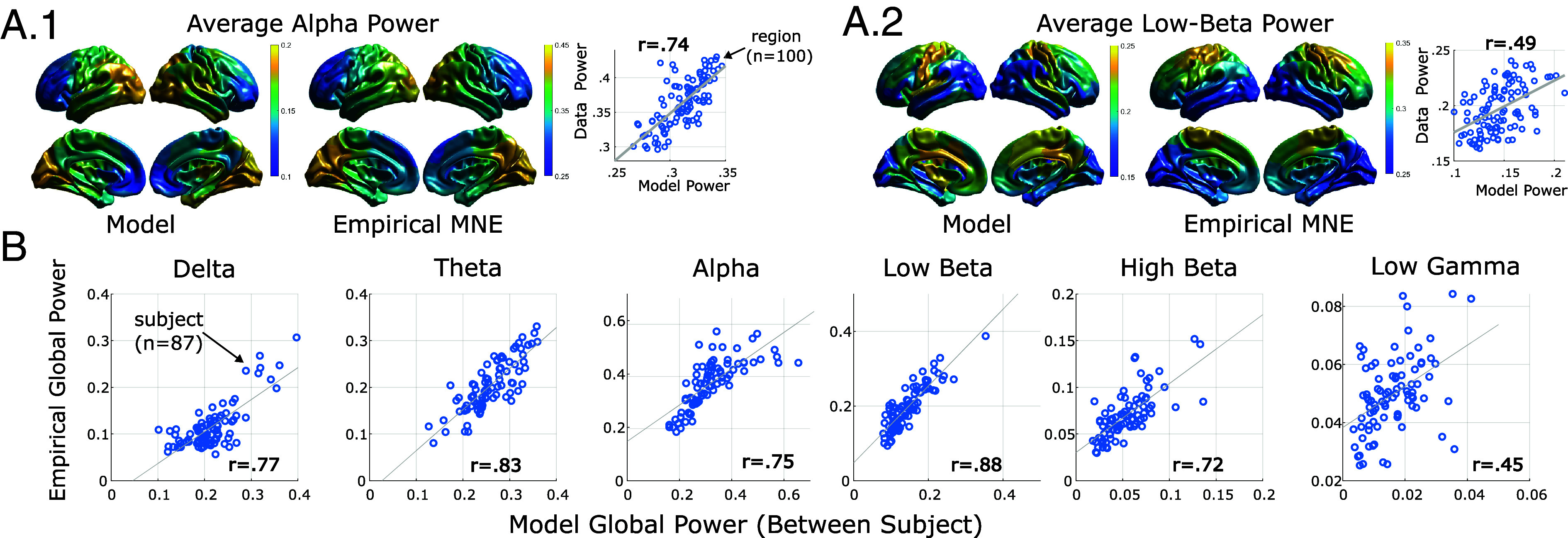
Precision brain models replicate empirical spatiospectral patterns. (A) Group-level anatomical distributions of spectral power strongly correlate between model-predictions and source-localized MEG for two of the stereotyped M/EEG bands at rest: alpha (A-1) and low-beta (A-2). (B) Individual differences in whole-brain spectral power (averaged over parcels) are reproduced across frequency bands by individualized brain models.
We first analyzed results at the group level by comparing the group-average anatomical profile of spectral power between model simulations and empirical estimates. Results demonstrate good spatial agreement for the alpha band (; Fig. 4 A-1) and moderate agreement for the beta bands (, , respectively; Fig. 4 A-2). We note that the model-predicted low-beta is highly localized to the somatomotor network, compared to the blurrier source-estimates. The slow delta band also exhibited high similarity between data and models (). By contrast, the theta band was moderately consistent: .
We next examined model fidelity in replicating oscillatory dynamic patterns. At the coarsest level, we found that models strongly reproduce individual differences in global spectral power (whole-brain average) across spectral bands in the training data (delta through high-beta: E-15, Fig. 4B). Interestingly, we also found a moderate correlation between individual differences in the low-gamma band (1.1E-5, Fig. 4B) despite its suppression in training-data due to 30 Hz low-pass filtering (excluding the full band). However, in contrast to other bands, the magnitude of model-predicted low-gamma power was significantly smaller than the HCP source-estimates and the average spatial profile was not consistent with data (), so this result may simply reflect residual gamma-power retained in training data even after filtering.
We also found that models replicated individual differences in spectral power at the network level for the main resting-state bands (alpha, low-beta). To compute network-level power, we averaged spectral power among parcels belonging to each of the 17 Yeo (53) resting-state networks as implemented in the Schaefer 100-17 network parcellation (55). We correlated model-predicted and empirical power in a multilevel model with a fixed-effect of subject (global power) collapsed across all networks. We found the strongest similarity between model-predictions and data for the alpha (), low-beta (), and delta () bands. While all statistical models were significant (due to the large number of data points), similarity was weak in the theta (), high-beta (), and gamma () bands. These results suggest that, for the main resting-state bands (alpha, low-beta), models correctly predict network-level power at the single subject level. However, despite high accuracy in predicting global power (see above), models are less accurate at predicting the anatomical/network sources of high-beta and theta-band power.
As a final validation, we examined whether models predict individual variation in the peak frequency of the alpha band. Empirically, this characterization has proven a remarkably stable and predictive measure of individual differences in brain and behavior (18, 56). The functional significance of “peak-alpha” is not yet resolved, although many accounts posit that the width of an alpha-oscillation determines the temporal window over which phase-linked processes (e.g., information integration) occur (19, 57). We found that models were accurate at reproducing the global individual alpha-frequencies (; Fig. 5A). At the parcel-level, we found that model accuracy was highest in predicting peak-alpha within the posterior cortex which agrees with the anatomical expression of alpha power (Fig. 5B).
Fig. 5.

Models predict individual’s peak frequency within the alpha band and explain individual differences in power. (A) Correlation between predicted and empirical global-peak alpha (average over parcels). (B) Model predictions of local peak frequency are most accurate in posterior regions in which the alpha rhythm is dominant. (C) Spearman correlation matrix between model parameters and global power in each frequency band. (D) Correlations between individual differences in the ratio of excitatory and inhibitory activity and global power by frequency band.
E-I Balance Predicts Individual Differences in Whole-Brain Average Spectral Power.
Generative models, as we present here, can form predictions using either overt linkages to model-parameters or as emergent phenomena generated by their dynamics. We therefore tested whether individual differences in spectral power or peak-alpha are correlated with individual parameters embedded in the models (Fig. 5C). Between subjects, we found that connections onto inhibitory populations (local , local , and distal ) had a strong negative correlation with alpha-power (’sE-6, respectively), and a positive correlation with beta-power (low beta: ’s3E-6, high-beta: ’s2E-8). This relationship also held for the excitatory decay-rate (alpha: , low-beta: , high-beta: ’sE-10) and was reversed for distal connections (alpha, , low-beta: , high-beta: , ’s6E-4). Relationships were similar to alpha, but weaker, in the theta band and similar to beta in the low-gamma band (Fig. 5C). These parameter-level relationships suggest that the global (i.e., whole-brain average) excitation–inhibition ratio changes spectral power in the low vs. high frequency bands.
Motivated by these parameter-level relationships, we quantified the model-predicted excitation–inhibition ratio for each parcel using the square-root ratio of power between and . This estimate was highly reliable (for brain-wide average: ) with much larger variation between-subject () than between-region (), hence we only further investigated the brain-wide average due to small anatomical variation. In agreement with the aforementioned parameters, the predicted EI-ratio was positively correlated with global alpha-power (, Fig. 5D), but negatively with beta power (low-beta: , high-beta: , ’s). Results thus indicate that individual differences in models’ excitation–inhibition ratio predict empirical power in the higher-frequency (but subgamma) frequency bands. This result is complementary, but not identical, to theoretical models suggesting a relationship between excitation–inhibition ratio and the slope of power-spectral density (58, 59). Interestingly, however, these relationships only held at the global scale. Neither the model-predicted excitation–inhibition ratio, nor the strength of distal connections (EE, EI) predicted the anatomical distribution of spectral power for any band (max , n.s.). The spatial gradient of local-recurrent connections was weakly correlated with gamma-band power , post-Bonferroni correction) and nonsignificant for all other bands. We did not find any significant relationships between model parameters/excitation–inhibition ratio and the peak alpha frequency in terms of individual differences or anatomy.
Thus, in total, individual model parameters strongly predict individual differences in global beta vs. alpha power, via the excitation–inhibition ratio. But, these parameters, in isolation, do not predict the anatomical profile of spectral power or the peak alpha frequency, even though these features are readily generated by the models (see above). Thus, the spatial distribution of spectral power is an emergent property generated by model dynamics as opposed to reflecting a singular parameter of the model.
Model Predicts the Existence of Individually Reliable Equilibrium and Nonequilibrium Oscillatory Dynamics.
Last, we used the models to interrogate the dynamical properties of two resting-state oscillations: alpha waves and beta waves (low-beta and high-beta). As previously mentioned, alpha rhythms (defined as 8 to 15 Hz for HCP, but more commonly 8 to 12 Hz) are high-amplitude posterior oscillations, often present at rest, which are amplified during eye closure and by tasks that require visual inhibition, broadly defined. While alpha constitutes one of the first-discovered waking-EEG components, theories regarding its origin and mechanism have evolved significantly over the past two decades. Initial theories, based upon the eye-closure effect, posited that alpha represented a default “cortical idling” state to which the visual system would return, absent environmental stimuli (see refs. 60 and 61 for review), potentially driven by thalamic nuclei (13, 14). By contrast, alpha activity is now largely interpreted through the lens of preparatory attention (62) and active visual inhibition (e.g. refs. 63 and 64). Several recent results have also indicated the potential for cortically initiated alpha waves to propagate retrograde along the dorsal visual pathway, from anterior (higher-order) to posterior (lower-order) cortex (15, 65), in addition to a visually evoked forward-propagating wave (65, 66).
We tested dynamical mechanisms by which alpha and beta waves could be generated at rest. From a theoretical perspective, there are several candidate mechanisms that can generate wave-like dynamics, including limit cycles (stable, periodic behavior that the system will recover after small perturbations), quasiperiodic behavior (mixed oscillations at incommensurable frequencies), aperiodic waves (e.g., spectrally concentrated chaos), stable foci/spiral-points (transient damped-oscillations when the system is perturbed), and noise-driven “switching” between different equilibrium states. As an initial investigation, we considered the attractor structure of the models, dividing models into those with equilibrium-style attractors and those with nonequilibrium attractors. The former class defines models which, in the absence of external perturbation, generate complex transient behavior, but will eventually settle into a steady state. The latter class of dynamics, converge onto low-dimensional patterns of persistent activity, such as oscillations, even without perturbation. The dynamics embedded near an attractor thus determine the system’s “default” mode of activity, whereas transient patterns of activity require some initial perturbation into that regime.
We found that these categories were consistent within-subject with of subjects having the same category for separate models fit to each data half (Odds Ratio 14.4, independence , ). Of the 87 subjects, 40 () belonged to the equilibrium group for both scans, 28 () belonged to the nonequilibrium group, and 19 () had one scan in each category (Fig. 6A). These groups did not differ in gender (, n.s.), although nonequilibrium subjects tender to be slightly younger (). For the three HCP age groups (22 to 25, 26 to 30, and 31 to 35), equilibrium subjects were split 4–17–20, respectively among age groups, whereas nonequilibrium subjects were split 9–12–7. However, due to the small sample size, these inferences are limited.
Fig. 6.

Models identify a taxonomy of subjects based upon attractor geometry. (A) Global power-spectral density for all subjects in which models were consistent in producing equilibrium or nonequilibrium dynamics. Left side shows example attractors for three subjects, one with an equilibrium spiral-point attractor (Top) and two with nonequilibrium attractors (a quasiperiodic torus on the left and limit-cycle on the right). All attractors are projected onto three-dimensional coordinates identified by PCA. Right side shows brainwide average power-spectral density by subject. (B) Band limited power for each group of subjects. (C) Models predict that attractor geometry is associated with alterations in local excitatory–inhibitory balance and timescales. (D) “Dimensionality” of model dynamics by attractor group as calculated using either participation-ratio dimension or thresholded-PCA (Materials and Methods). (E) Models predict that alpha oscillations become faster (higher-peak frequency) under perturbation. Shading indicates 1 SE (). (F) Group-level bifurcation plot for rescaling (multiplying) the EI and II connection strengths. Plots indicate the percent of subjects generating nonequilibrium dynamics for those parameter changes and are separated by subjects generating equilibrium vs. nonequilibrium dynamics in the base model. Base models are at the center of the red cross.
Surprisingly, these categories proved powerful markers of individual differences in empirical spectral power. We observed strong increases in alpha and theta power, but decreases in beta and low-gamma power for subjects with nonequilibrium dynamics (theta: , alpha: , low-beta: , high-beta: , low-gamma: , ’s0.0008) (Fig. 6B). In an agreement with the group-wide parameter-correlation results (Fig. 5), we found that equilibrium (low-alpha) subjects had an increase in EI connection strength leading to a lower ratio of excitatory-to-inhibitory activity (Fig. 6 C1) and changes in the integration time-constants (Fig. 6 C2). As before, we found contrasting influences of the strength and inhibitory decay parameter; however, the net influence, over relevant ranges of activity, was an increase in negative feedback (faster decay) for the equilibrium subjects, particularly near the equilibrium (where ’ is particularly large). However, there was no difference between groups for the empirical peak-alpha frequency (, n.s.). These results suggest that some aspect of the low-dimensional attractors promote the generation of high-amplitude oscillations in a band-selective manner as opposed to globally speeding/slowing dynamics (which would be reflected in peak frequency).
Alpha Oscillations Arise from Low-Dimensional Dynamics and Are Sensitive to Perturbation.
We further considered how the induced dimension of model dynamics affects the alpha rhythm. Here, we are interested in the effective dimension of the stochastic (noisy) dynamics, i.e., how expressive are the models in terms of spatial activity patterns under physiological conditions. For this test, we used two different component-based measures of dimensionality for comparison: a hard-threshold dimension based upon the number of nontrivial PCA components (, threshold = ) and the Participation Ratio Dimension (; see Materials and Methods) which is a graded measure. We did not use topological definitions (e.g., Hausdorff dimension) as we were interested in global dynamics embedded within the high-dimensional space, as opposed to only studying the attractors. Results indicated lower induced-dimension for nonequilibrium subjects (, ) compared with equilibrium subjects (, ) as assessed with two-sample t-tests corrected for unequal variance (, , , ; Fig. 6D). These findings agree with previous, empirical descriptions of lower-dimensional dynamics associated with alpha band vs. beta (67) activity. This analysis indicates that the lower-dimensional dynamics which embed nonequilibrium attractors, contract dynamics throughout the state-space, rather than solely in the vicinity of the attractor. Thus, the global dynamics of nonequilibrium subjects are shaped by lower-dimensional structures.
To clarify the association of low-dimensional/ nonequilibrium dynamics with spectral power, we investigated how the models reacted to perturbations. This analysis is important for interrogating whether the alpha rhythm is, itself, an attractor (e.g., limit-cycle) or rather reflects transient behavior built upon the nearby dynamics. For this analysis, we focused upon changes within the alpha spectra, as opposed to between spectra. We also emphasize high-level properties, as opposed to simulating a specific task, so we modeled environmental perturbations as a random process independently delivered to each brain area. The perturbation magnitude is thus equivalent to the noise-level which we applied as a scaling factor to simulated physiological/process noise (with baseline covariance as estimated by individual models). As before, process noise denotes stochasticity which drives a system, as opposed to artifact which only appears in measurements. We scaled noise-perturbations variance from a factor of 0.002 to 0.1 with resolution 0.001 and 0.1 being the value used in previously presented simulations. Averaging over subjects, we found that the peak alpha frequency within the visual network linearly increased as a function of perturbation strength (, ; Fig. 6E). This effect agrees with empirical findings of the peak alpha frequency changing within-subject, depending upon the level of engagement [increases during task, (18, 19)] and has been explored as a generic property in previous theoretical models (68, 69). We also note the observed change in peak frequency indicates inherently nonlinear dynamics, so the existence of an equilibrium attractor should not be confused with approximately linear dynamics. Together, these demonstrations indicate the potential of our framework to inform high-level systems neuroscience and implicate mechanisms of person-driven and context-driven variation.
Models Enable Topological Predictions at the Individual Level.
Last, we examined whether an explicit bifurcation mechanism explains how individual variability in mechanistic model parameters determines attractor structure. Based upon our finding that equilibrium vs. nonequilibrium subjects primarily differed in terms of local-circuit parameters, we focused our analysis upon the parameters describing local circuits: EE,EI,IE, and II strength. Previous literature has primarily studied these features in terms of group-level or normative models (e.g., ref. 32), while we perform our analysis at the individual level. We developed separate bifurcation landscapes for equilibrium and nonequilibrium subjects and report parameter changes in relative units (rescaling relative to baseline value) to facilitate cross-subject inferences (Fig. 6F). This analysis revealed two insights. First, the bifurcation landscape is consistent within attractor group, meaning that the points of crossover from equilibrium to nonequilibrium dynamics are conserved within members of the same group. This fact is especially apparent in the equilibrium subject group in which there were sharp boundaries between parameter settings in which and of models generated nonequilibrium dynamics. Second, although equilibrium subjects had relatively higher values for both EI and II connection strength, these effects could counteract. Further increasing the value, alone, actually promotes nonequilibrium dynamics (Fig. 6F) and there exists a clear boundary between attractor classes such that increasing relative promotes nonequilibrium dynamics and vice versa. Such inferences would not be possible without a generative model on which to perform bifurcation analysis. Indeed, looking at parameter values, in isolation, would lead to the incorrect conclusion that increasing , in isolation, promotes equilibrium dynamics.
Interpreting Attractor Groups.
In this paper, we have identified a reliable differentiation among subjects based upon model attractor topology which we divide into subjects with only equilibrium-type attractors and those which also generated nonequilibrium attractors. However, while these structures are useful for inferring patterns of global dynamics, the model’s predictions, under internal noise, need not obey a single behavior. Previous literature (70–72) has referenced a bimodal distribution of alpha power in eyes-closed resting state as evidence of two stable states. We attempted to test this phenomenon in the HCP data, which is eyes-open, and models using the same analysis. However, we did not find pronounced bimodal peaks in the alpha-power histogram of HCP resting-state data (SI Appendix). Likewise, model simulations also generated a unimodal distribution of alpha-power over time, even in cases where the model possessed multiple attractors. We believe this difference may be the result of HCP using an eyes-open paradigm, in contrast to the eyes-closed data reported in other studies (70, 71). Posterior alpha-power is more pronounced in the eyes-closed state, which may explain the ability to detect two peaks. By contrast, if state switches were present in our data/models, it may be that they were either too brief or too low amplitude to be distinguished from the tail-end of a single-state system. We did not attempt to dissociate states based solely upon changes in the distribution skewness as this feature could also be attributed to violations of Gaussianity assumptions.
Discussion
Enabling Data-Driven Modeling at Whole-Brain Scales.
We have presented a framework for estimating precision brain models from single-subject M/EEG data. Our gBPKF algorithm is shown highly capable of solving the dual-estimation problems inherent in direct brain modeling and reliably estimates latent brain model parameters directly from M/EEG timeseries. Importantly, we stress that our approach directly applies nonlinear system identification to macroscale cortical activity, seeking to solve for the system’s vector field (i.e., the moment-to-moment variation) as opposed to replicating a specific signal feature. Nonetheless, our approach reproduces the spatial distributions and individual differences in band-limited power across the main M/EEG bands with high fidelity. The models also link individual differences in alpha power to the geometry of underlying dynamics as shaped by excitatory–inhibitory balance. These applications demonstrate the inferential power of individualized (precision) brain modeling.
Limitations.
We view our present model as having two primary limitations: 1) assumptions regarding how the M/EEG signal is generated and 2) the omission of subcortical sources and other biological details. We stress that these limitations are features of our current model (two nodes per cortical parcel) rather than the approach per se. We have designed our publicly available code so that it is easy to implement arbitrary models of neural circuitry and M/EEG signal weighting (with the usual trade-offs between run-time/robustness and model complexity). We therefore examine some of our model’s limitations with the caveat that these limitations are not inherent to our general estimation approach (gBPKF). In the first limitation, we make the typical assumption that current-dipoles reflect excitatory neuron depolarization and that the dipole, like the cells themselves, is oriented normal to the cortical surface. While convenient, these assumptions are not always valid (37, 73) so further refinement of the measurement matrix () may improve anatomical precision.
A second limitation arises from the neglect of subcortical influences. In the current work, we chose to only model cortex, in line with the predominantly cortical origin of M/EEG signals. However, interactions with the brainstem, thalamus, and hippocampus are known to generate many slow EEG components. It is for this reason that our frequency-domain validations focused upon the faster alpha and beta bands, although the cortical vs. subcortical origins of either phenomena are not yet settled, although see ref. 15. In any case, it is clear that subcortical influences certainly guide cortical dynamics and that their inclusion could improve model performance. Several dynamic causal modeling approaches, for instance, have included subcortical regions in modeling M/EEG (5, 74). This approach usually requires strong priors as the optimization may otherwise become ill-posed.
We have first prioritized validating our framework within an empirically verifiable model space, as opposed to including as many degrees of freedom as possible. It is therefore possible that some of the would-be explanatory variance associated with cortico-thalamo-cortical pathways is mismodeled in our approach as direct cortico-cortical connections in the absence of a subcortical component. However, we have designed our modeling approach such that subcortical regions can be easily added with or without various priors as another latent variable, treated analogously to the interneurons (). We encourage (verifiable) expansion in this direction.
Relationship and Comparisons with Prior Whole-Brain Modeling Frameworks.
We have described at several points above the relationship of dual MINDy to prior approaches in large-scale and whole-brain data-driven modeling, but it is worth elaborating on a few of the key conceptual and methodological distinctions. In particular, model-inversion approaches in neural field theory (NFT) provide an alternative means to parameterize even more detailed mechanisms at the biological level, such as the shape of postsynaptic potentials, multiple subcortical populations, and a thalamocortical delay (46, 47, 70, 71, 75, 76). These methods leverage a linear approximation of the underlying dynamics which provides an explicit link to the predicted power-spectral density (PSD) under idealized noise statistics. As NFT models are directly fit to PSD, they reproduce the estimated spectra with negligible error. Our model predictions of PSD, while a reasonable approximation, are qualitatively lower than those generated by NFT models estimated from PSD. NFT approaches have been successful in generating fundamental dynamical insights into brain mechanisms, including the nature of bistability and wave propagation in the cortex, e.g. refs. 72 and 75.
By contrast, our approach derives from the perspective of local and long-distance brain connectivity as region-dependent (29, 32). This generates a very large number of unknown parameters compared to modeling the cortex as a continuum, while our embrace of nonlinearity also means that the model parameters do not have an analytic mapping onto power-spectral density. These tradeoffs are important considerations when weighing the benefits of neural field theory vs. heterogeneous neural masses. They are also important when contemplating the appropriate ways to compare or benchmark approaches. For instance, the analytical intractability of the PSD with respect to dual MINDy means that we cannot directly use this as an objective function. Likewise, the fully Bayesian approaches utilized for estimation in the Virtual Brain will not scale to the number of parameters we are using in dual MINDy. Thus, to enact an apples-to-apples comparison would require nontrivial modifications to dual MINDy, or likewise modifying in fundamental ways the prior approaches (e.g., to perform estimation in the time-domain). We do advocate the importance of identifying objective, methodology-independent benchmarks within the community (e.g., such as in the machine learning field). Both predictive measures (both within and out of distribution) as well as reliability of individual differences metrics may be candidates, and we encourage an engagement of this issue in the future.
Conclusions.
In conclusion, we have validated an approach for precision brain modeling using single-subject M/EEG and illustrated its explanatory potential in the context of resting-state oscillations. We hope that these innovations will enable insight into individual variation and circuit mechanisms that may, eventually, inform ways of interacting with the brain (e.g., neurostimulation).
Materials and Methods
In this section, we briefly describe the resting-state magnetoencephalography (MEG) data used for model training and validation. An introduction to the Kalman Filter and details of the gBPKF algorithm are presented in SI Appendix. Technical descriptions of ground-truth model generation are also provided in SI Appendix.
HCP MEG Data Processing.
Models were fit to MEG data provided by the Human Connectome Project [HCP; (38)]. We used the minimally preprocessed HCP pipeline for MEG which centers on using independent component analysis (ICA) to identify and remove artifact.
We then projected data according to the left singular-vectors of the leadfield matrix (derived from the precalculated Boundary Element Method headmodels). This step corresponds to reducing dimensionality based upon what spatial patterns MEG can measure as opposed to those that were observed (in practice these approaches overlap). Our criterion was to only retain leadfield dimensions (singular vectors whose singular values were % of the maximum singular value. These reductions were done on a per-scan basis, which meant that, due to the removal of bad channels, projections (hence measurement models) often differed between scans of the same subject.
Frequency-Domain Filtering.
Data were filtered between the delta and high-beta bands (1.3 to 30 Hz). The 30 Hz upper limit marks the high-beta band while the 1.3 Hz lower limit was adopted from the HCP ICA processing pipeline and does not include the full delta-band (i.e., is above the slowest delta waves). This range also includes the full alpha and theta-bands. As part of the HCP MEG pipeline, high-artifact data segments are automatically removed, resulting in variable length segments of good-quality data. To calculate power spectral density (PSD) at the subject level, we first discarded segments lasting less than 20 s. The PSD was then calculated for each timeseries and discretized with resolution 0.25 Hz. The resultant PSDs were averaged across segments, weighted according to segment length.
For band-limited power, we used the precalculated HCP estimates in the ICA-MNE pipeline. This pipeline solves for a full dipole-vector timeseries at each of the 8,004 vertices (three dipole coordinates per vertex). Band-limited power is estimated by filtering the timeseries for each dipole coordinate and then calculating the squared magnitude of the filtered dipole vectors. HCP defines eight specific bands: delta, theta, alpha, low-beta, high-beta, and low/mid/high gamma. In the presented results, we normalized the average band-limited power at each dipole by the whole-spectrum (unfiltered) power and then averaged within parcel to get parcel-level power.
ICA Artifact Detection.
We used the HCP MEG-ICA pipeline to identify artifactual independent components (ICs). The HCP MEG2 and later releases sort large ICs as having a brain or nonbrain origin. However, whereas the original ICA pipeline retained only “brain” ICs (removing both artifactual and low-variance ICs), we simply removed the nonbrain ICs by orthogonal projection, thereby retaining the original channel dimensions. This step retains information that the low-variance ICs are measurable and small, whereas removing them would imply that those dimensions are unmeasurable (potentially leading to model overfit). Denoting the ICA mixing matrix for the bad ICs as and the post-ICA corrected measurements :
| [7] |
Source Localization.
We used the standard HCP anatomical pipeline to compute forward head models. Comparisons with empirical source-level power all used the HCP precalculated power-distributions which allow full 3d dipole configurations (38). However, model-training requires a fixed mapping between activity patterns and measurements, and thus a single, constant, dipole orientation per vertex (up to sign reversal). We reduced the 3d forward model to a single dipole direction per vertex by assuming that dipoles are oriented normal to the cortical surface (as calculated in FieldTrip using the vertex cross-product method). In order to transform MEG magnetometer/gradiometer measurements onto cortical dipoles we used minimum norm estimation [MNE; (77)]. Like other linear source-localizers, The MNE inverse matrix maps sensor-level data onto the brain:
| [8] |
Conceptually, MNE minimizes the expected mean-square-error (like the Kalman Filter) and therefore takes the regression form:
| [9] |
Following the HCP ICA-MNE pipeline, we use the simplified assumption that and are each independent and identically distributed (iid) hence, using the noise-signal-ratio (NSR) coefficient :
| [10] |
We calculated analogous to the HCP minimal pipeline, but with a single per run, applied in channel-space, whereas the HCP rescaled ’s for each IC. This difference is due to retaining the original channel space, instead of reducing dimensionality to ICs.
| [11] |
with noise-value factor . The inverse solution was calculated separately for each resting-state run and potentially differed (e.g., due to noisy channel removal). We further rescaled each row of to produce unit variance in which was done separately for each run.
Statistical Analysis.
Our analyses were of three categories: 1) validating/benchmarking the approach with a known (simulated) ground truth, 2) assessing reliability with real-world data, and 3) exploring dynamical predictions made by the models. For these analyses, we used three similarity measures depending upon the variable’s dimensionality. We used simple correlation (collapsing over nonmasked connections) to gauge the overall similarity of two matrices/vectors. To assess the reliability of individual differences, we used intraclass correlation (78) for scalar-valued parameters (e.g., time constants) and image intraclass correlation [I2C2; (54)] for multivariate parameters (e.g., connectivity). All reported -values are two-tailed. Multiple-comparison corrections all used the Bonferroni method and statistics reported as significant all passed this threshold. We use the notation for calculated values less than as exact estimates are likely inaccurate past this point. When multiple related analyses are presented in-text, we typically report the largest -value over all of the analyses with the notation , to improve readability.
Quantifying Dimensionality.
We quantified dimensionality of stochastic dynamics in two ways, both based off of the covariance eigenspectrum, with convergent results. First, we used the PCA-threshold method with a hard-boundary defined by of the maximal component weight (eigenvalue). For this method, we quantified dimensionality as the number of components passing this threshold. For comparison, we used the participation ratio dimension (79, 80) which is calculated from the covariance eigenvalues ():
| [12] |
We used for comparison as it provides a soft dimensionality metric in terms of the variance spread as opposed to being premised upon a single, low-dimensional surface. It is also sensitive to dynamics which are nontrivial in the stochastic case, but eventually converge in the absence of noise. We present calculated using z-scored simulated data (i.e., using correlation instead of covariance) to control for the different scaling of excitatory and inhibitory neurons. However, statistical inferences led to the same conclusion with/without normalization.
Supplementary Material
Appendix 01 (PDF)
Acknowledgments
M.F.S. was funded by NSF-DGE-1143954 from the US NSF, the McDonnell Center for Systems Neuroscience, and NIH T32 DA007261-29 from the National Institute on Drug Addiction. Portions of this work were supported by NSF 1653589 and NSF 1835209 (S.C.), from the US NSF, NINDS R01NS130693 (S.C.), and NIMH R21MH132240 (T.S.B.).
Author contributions
M.F.S., T.S.B., M.C., and S.C. designed research; M.F.S. performed research; M.F.S. contributed new tools; M.F.S. analyzed data; and M.F.S., T.S.B., M.C., and S.C. wrote the paper.
Competing interests
The authors declare no competing interest.
Footnotes
This article is a PNAS Direct Submission.
Data, Materials, and Software Availability
The resting-state MEG data used for model-building and analysis are publicly available through the Human Connectome Project [HCP; (38)]. They can be accessed, through a registered account, at db.humanconnectome.org. Data processing code, as described below, is available through HCP. Interested users should download the “megconnectome” pipeline scripts through the HCP database: https://www.humanconnectome.org/software/hcp-meg-pipelines. A software package containing MATLAB code for gBPKF model-fitting, simulation, and visualizing results is available at the primary author’s GitHub: https://github.com/singhmf/MINDy-BPKF.
Supporting Information
References
- 1.Gratton C., et al. , Functional brain networks are dominated by stable group and individual factors, not cognitive or daily variation. Neuron 98, 439–452 (2018). [DOI] [PMC free article] [PubMed] [Google Scholar]
- 2.Ritter P., Schirner M., McIntosh A. R., Jirsa V. K., The virtual brain integrates computational modeling and multimodal neuroimaging. Brain Connect. 3, 121–145 (2013). [DOI] [PMC free article] [PubMed] [Google Scholar]
- 3.Jirsa V., et al. , The virtual epileptic patient: Individualized whole-brain models of epilepsy spread. Neuroimage 145, 377–388 (2017). [DOI] [PubMed] [Google Scholar]
- 4.Friston K., Harrison L., Penny W., Dynamic causal modelling. Neuroimage 19, 1273–1302 (2003). [DOI] [PubMed] [Google Scholar]
- 5.Kiebel S. J., Garrido M. I., Moran R. J., Friston K. J., Dynamic causal modelling for EEG and MEG. Cogn. Neurodyn. 2, 121–136 (2008). [DOI] [PMC free article] [PubMed] [Google Scholar]
- 6.Razi A., Seghier M. L., Zhou Y., McColgan P., Large-scale DCMs for resting-state fMRI. Network Neurosci. 1, 222–241 (2017). [DOI] [PMC free article] [PubMed] [Google Scholar]
- 7.Stam C. J., Nonlinear dynamical analysis of EEG and MEG: Review of an emerging field. Clin. Neurophysiol. 116, 2266–2301 (2005). [DOI] [PubMed] [Google Scholar]
- 8.Lo M. T., Tsai P. H., Lin P. F., Lin C., Hsin Y. L., The nonlinear and nonstationary properties in EEG signals: Probing the complex fluctuations by Hilbert–Huang transform. Adv. Adapt. Data Anal. 1, 461–482 (2009). [Google Scholar]
- 9.Kondacs A., Szabó M., Long-term intra-individual variability of the background EEG in normals. Clin. Neurophysiol. 110, 1708–1716 (1999). [DOI] [PubMed] [Google Scholar]
- 10.Braver T. S., Cole M. W., Yarkoni T., Vive les differences! Individual variation in neural mechanisms of executive control Curr. Opin. Neurobiol. 20, 242–250 (2010). [DOI] [PMC free article] [PubMed] [Google Scholar]
- 11.Sun L., Peräkylä J., Hartikainen K. M., Frontal alpha asymmetry, a potential biomarker for the effect of neuromodulation on brain’s affective circuitry–preliminary evidence from a deep brain stimulation study. Front. Hum. Neurosci. 11, 584 (2017). [DOI] [PMC free article] [PubMed] [Google Scholar]
- 12.Lozano-Soldevilla D., On the physiological modulation and potential mechanisms underlying parieto-occipital alpha oscillations. Front. Comput. Neurosci. 12, 23 (2018). [DOI] [PMC free article] [PubMed] [Google Scholar]
- 13.Da Silva F. L., Van Lierop T., Schrijer C., Van Leeuwen W. S., Organization of thalamic and cortical alpha rhythms: Spectra and coherences. Electroencephalogr. Clin. Neurophysiol. 35, 627–639 (1973). [DOI] [PubMed] [Google Scholar]
- 14.Schreckenberger M., et al. , The thalamus as the generator and modulator of EEG alpha rhythm: A combined PET/EEG study with lorazepam challenge in humans. Neuroimage 22, 637–644 (2004). [DOI] [PubMed] [Google Scholar]
- 15.Halgren M., et al. , The generation and propagation of the human alpha rhythm. Proc. Natl. Acad. Sci. U.S.A. 116, 23772–23782 (2019). [DOI] [PMC free article] [PubMed] [Google Scholar]
- 16.Feshchenko V. A., Veselis R. A., Reinsel R. A., Propofol-induced alpha rhythm. Neuropsychobiology 50, 257–266 (2004). [DOI] [PubMed] [Google Scholar]
- 17.Connemann B. J., et al. , Anterior limbic alpha-like activity: A low resolution electromagnetic tomography study with lorazepam challenge. Clin. Neurophysiol. 116, 886–894 (2005). [DOI] [PubMed] [Google Scholar]
- 18.Haegens S., Cousijn H., Wallis G., Harrison P. J., Nobre A. C., Inter- and intra-individual variability in alpha peak frequency. Neuroimage 92, 46–55 (2014). [DOI] [PMC free article] [PubMed] [Google Scholar]
- 19.Cecere R., Rees G., Romei V., Individual differences in alpha frequency drive crossmodal illusory perception. Curr. Biol. 25, 231–235 (2015). [DOI] [PMC free article] [PubMed] [Google Scholar]
- 20.Drewes J., Muschter E., Zhu W., Melcher D., Individual resting-state alpha peak frequency and within-trial changes in alpha peak frequency both predict visual dual-pulse segregation performance. Cereb. Cortex 32, 5455–5466 (2022). [DOI] [PMC free article] [PubMed] [Google Scholar]
- 21.Vespa P. M., et al. , Early and persistent impaired percent alpha variability on continuous electroencephalography monitoring as predictive of poor outcome after traumatic brain injury. J. Neurosurg. 97, 84–92 (2002). [DOI] [PubMed] [Google Scholar]
- 22.Trammell J. P., MacRae P. G., Davis G., Bergstedt D., Anderson A. E., The relationship of cognitive performance and the theta-alpha power ratio is age-dependent: An EEG study of short term memory and reasoning during task and resting-state in healthy young and old adults. Front. Aging Neurosci. 9, 364 (2017). [DOI] [PMC free article] [PubMed] [Google Scholar]
- 23.Bentes C., et al. , Quantitative EEG and functional outcome following acute ischemic stroke. Clin. Neurophysiol. 129, 1680–1687 (2018). [DOI] [PubMed] [Google Scholar]
- 24.Arns M., EEG-based personalized medicine in ADHD: Individual alpha peak frequency as an endophenotype associated with nonresponse. J. Neurother. 16, 123–141 (2012). [Google Scholar]
- 25.Başar E., Başar-Eroğlu C., Güntekin B., Yener G. G., Brain’s alpha, beta, gamma, delta, and theta oscillations in neuropsychiatric diseases: Proposal for biomarker strategies. Suppl. Clin. Neurophysiol. 62, 19–54 (2013). [DOI] [PubMed] [Google Scholar]
- 26.Renauld E., Descoteaux M., Bernier M., Garyfallidis E., Whittingstall K., Semi-automatic segmentation of optic radiations and LGN, and their relationship to EEG alpha waves. PLoS ONE 11, e0156436 (2016). [DOI] [PMC free article] [PubMed] [Google Scholar]
- 27.Honey C. J., et al. , Predicting human resting-state functional connectivity from structural connectivity. Proc. Natl. Acad. Sci. U.S.A. 106, 2035–2040 (2009). [DOI] [PMC free article] [PubMed] [Google Scholar]
- 28.Schirner M., Rothmeier S., Jirsa V. K., McIntosh A. R., Ritter P., An automated pipeline for constructing personalized virtual brains from multimodal neuroimaging data. Neuroimage 117, 343–357 (2015). [DOI] [PubMed] [Google Scholar]
- 29.Demirtaş M., et al. , Hierarchical heterogeneity across human cortex shapes large-scale neural dynamics. Neuron 101, 1181–1194 (2019). [DOI] [PMC free article] [PubMed] [Google Scholar]
- 30.Neymotin S. A., et al. , Human neocortical neurosolver (HNN), a new software tool for interpreting the cellular and network origin of human meg/eeg data. eLife 9, e51214 (2020). [DOI] [PMC free article] [PubMed] [Google Scholar]
- 31.Honey C. J., Kötter R., Breakspear M., Sporns O., Network structure of cerebral cortex shapes functional connectivity on multiple time scales. Proc. Natl. Acad. Sci. U.S.A. 104, 10240–10245 (2007). [DOI] [PMC free article] [PubMed] [Google Scholar]
- 32.Wang P., et al. , Inversion of a large-scale circuit model reveals a cortical hierarchy in the dynamic resting human brain. Sci. Adv. 5, eaat7854 (2019). [DOI] [PMC free article] [PubMed] [Google Scholar]
- 33.Domhof J. W., Eickhoff S. B., Popovych O. V., Reliability and subject specificity of personalized whole-brain dynamical models. Neuroimage 257, 119321 (2022). [DOI] [PubMed] [Google Scholar]
- 34.Brunel N., Wang X. J., What determines the frequency of fast network oscillations with irregular neural discharges? I. Synaptic dynamics and excitation-inhibition balance. J. Neurophysiol. 90, 415–430 (2003). [DOI] [PubMed] [Google Scholar]
- 35.Atallah B. V., Scanziani M., Instantaneous modulation of gamma oscillation frequency by balancing excitation with inhibition. Neuron 62, 566–577 (2009). [DOI] [PMC free article] [PubMed] [Google Scholar]
- 36.van Kerkoerle T., et al. , Alpha and gamma oscillations characterize feedback and feedforward processing in monkey visual cortex. Proc. Natl. Acad. Sci. U.S.A. 111, 14332–14341 (2014). [DOI] [PMC free article] [PubMed] [Google Scholar]
- 37.Buzsáki G., Anastassiou C. A., Koch C., The origin of extracellular fields and currents—EEG, ECOG, LFP and spikes. Nat. Rev. Neurosci. 13, 407–420 (2012). [DOI] [PMC free article] [PubMed] [Google Scholar]
- 38.Larson-Prior L. J., et al. , Adding dynamics to the human connectome project with MEG. Neuroimage 80, 190–201 (2013). [DOI] [PMC free article] [PubMed] [Google Scholar]
- 39.Singh M. F., Braver T. S., Cole M. W., Ching S., Estimation and validation of individualized dynamic brain models with resting state fMRI. Neuroimage 221, 117046 (2020). [DOI] [PMC free article] [PubMed] [Google Scholar]
- 40.Singh M., Wang A., Braver T., Ching S., Scalable surrogate deconvolution for identification of partially-observable systems and brain modeling. J. Neural Eng. 17, 046025 (2020). [DOI] [PMC free article] [PubMed] [Google Scholar]
- 41.Singh M. F., Wang A., Cole M., Ching S., Braver T. S., Enhancing task fMRI preprocessing via individualized model-based filtering of intrinsic activity dynamics. Neuroimage 247, 118836 (2021). [DOI] [PMC free article] [PubMed] [Google Scholar]
- 42.Wilson H. R., Cowan J. D., Excitatory and inhibitory interactions in localized populations of model neurons. Biophys. J. 12, 1–24 (1972). [DOI] [PMC free article] [PubMed] [Google Scholar]
- 43.Freestone D. R., et al. , A data-driven framework for neural field modeling. Neuroimage 56, 1043–1058 (2011). [DOI] [PubMed] [Google Scholar]
- 44.Freestone D. R., et al. , Estimation of effective connectivity via data-driven neural modeling. Front. Neurosci. 8, 383 (2014). [DOI] [PMC free article] [PubMed] [Google Scholar]
- 45.Rajabioun M., Nasrabadi A. M., Shamsollahi M. B., Estimation of effective brain connectivity with dual Kalman filter and EEG source localization methods. Australas. Phys. Eng. Sci. Med. 40, 675–686 (2017). [DOI] [PubMed] [Google Scholar]
- 46.Robinson P. A., et al. , Neurophysical modeling of brain dynamics. Neuropsychopharmacology 28, S74–S79 (2003). [DOI] [PubMed] [Google Scholar]
- 47.Robinson P. A., Rennie C. J., Rowe D. L., O’Connor S. C., Estimation of multiscale neurophysiologic parameters by electroencephalographic means. Hum. Brain Mapp. 23, 53–72 (2004). [DOI] [PMC free article] [PubMed] [Google Scholar]
- 48.M. F. Singh, M. Wang, M. W. Cole, S. Ching, “Efficient identification for modeling high-dimensional brain dynamics” in 2022 American Control Conference (ACC) (IEEE, 2022), pp. 1353–1358.
- 49.S. J. Julier, J. K. Uhlmann, “New extension of the Kalman filter to nonlinear systems” in Signal Processing, Sensor Fusion, and Target Recognition VI, I. Kadar, Ed. (SPIE, Bellingham, WA, 1997), vol. 3068, pp. 182–193.
- 50.Julier S., Uhlmann J., Durrant-Whyte H. F., A new method for the nonlinear transformation of means and covariances in filters and estimators. IEEE Trans. Autom. Control 45, 477–482 (2000). [Google Scholar]
- 51.Haarnoja T., Ajay A., Levine S., Abbeel P., Backprop KF: Learning discriminative deterministic state estimators. Adv. Neural. Inf. Process. Syst. 29, 1–9 (2016). [Google Scholar]
- 52.Finn E. S., et al. , Functional connectome fingerprinting: Identifying individuals using patterns of brain connectivity. Nat. Neurosci. 18, 1664–1671 (2015). [DOI] [PMC free article] [PubMed] [Google Scholar]
- 53.Thomas Yeo B. T., et al. , The organization of the human cerebral cortex estimated by intrinsic functional connectivity. J. Neurophysiol. 106, 1125–1165 (2011). [DOI] [PMC free article] [PubMed] [Google Scholar]
- 54.Shou H., et al. , Quantifying the reliability of image replication studies: The image intraclass correlation coefficient (I2C2). Cogn., Affect., Behav. Neurosci. 13, 714–724 (2013). [DOI] [PMC free article] [PubMed] [Google Scholar]
- 55.Schaefer A., et al. , Local–global parcellation of the human cerebral cortex from intrinsic functional connectivity MRI. Cereb. Cortex 28, 3095–3114 (2017). [DOI] [PMC free article] [PubMed] [Google Scholar]
- 56.Grandy T. H., et al. , Peak individual alpha frequency qualifies as a stable neurophysiological trait marker in healthy younger and older adults. Psychophysiology 50, 570–582 (2013). [DOI] [PubMed] [Google Scholar]
- 57.Klimesch W., Evoked alpha and early access to the knowledge system: The P1 inhibition timing hypothesis. Brain Res. 1408, 52–71 (2011). [DOI] [PMC free article] [PubMed] [Google Scholar]
- 58.Gao R., Peterson E. J., Voytek B., Inferring synaptic excitation/inhibition balance from field potentials. Neuroimage 158, 70–78 (2017). [DOI] [PubMed] [Google Scholar]
- 59.Lombardi F., Herrmann H. J., de Arcangelis L., Balance of excitation and inhibition determines 1/F power spectrum in neuronal networks. Chaos 27, 047402 (2017). [DOI] [PubMed] [Google Scholar]
- 60.Pfurtscheller G., Stancak A. Jr., Neuper C., Event-related synchronization (ERS) in the alpha band—An electrophysiological correlate of cortical idling: A review. Int. J. Psychophysiol. 24, 39–46 (1996). [DOI] [PubMed] [Google Scholar]
- 61.Cooper N. R., Croft R. J., Dominey S. J., Burgess A. P., Gruzelier J. H., Paradox lost? Exploring the role of alpha oscillations during externally vs. internally directed attention and the implications for idling and inhibition hypotheses. Int. J. Psychophysiol. 47, 65–74 (2003). [DOI] [PubMed] [Google Scholar]
- 62.Foxe J. J., Simpson G. V., Ahlfors S. P., Parieto-occipital 10 Hz activity reflects anticipatory state of visual attention mechanisms. NeuroReport 9, 3929–3933 (1998). [DOI] [PubMed] [Google Scholar]
- 63.Klimesch W., Sauseng P., Hanslmayr S., EEG alpha oscillations: The inhibition-timing hypothesis. Brain Res. Rev. 53, 63–88 (2007). [DOI] [PubMed] [Google Scholar]
- 64.Klimesch W., Evoked alpha and early access to the knowledge system: The P1 inhibition timing hypothesis. Brain Res. 1408, 52–71 (2011). [DOI] [PMC free article] [PubMed] [Google Scholar]
- 65.Alamia A., Terral L., D’ambra M. R., VanRullen R., Distinct roles of forward and backward alpha-band waves in spatial visual attention. eLife 12, e85035 (2023). [DOI] [PMC free article] [PubMed] [Google Scholar]
- 66.Lozano-Soldevilla D., VanRullen R., The hidden spatial dimension of alpha: 10-Hz perceptual echoes propagate as periodic traveling waves in the human brain. Cell Rep. 26, 374–380.e4 (2019). [DOI] [PMC free article] [PubMed] [Google Scholar]
- 67.Aftanas L., Golocheikine S., Non-linear dynamic complexity of the human EEG during meditation. Neurosci. Lett. 330, 143–146 (2002). [DOI] [PubMed] [Google Scholar]
- 68.Hutt A., Mierau A., Lefebvre J., Dynamic control of synchronous activity in networks of spiking neurons. PLoS ONE 11, e0161488 (2016). [DOI] [PMC free article] [PubMed] [Google Scholar]
- 69.Mierau A., Klimesch W., Lefebvre J., State-dependent alpha peak frequency shifts: Experimental evidence, potential mechanisms and functional implications. Neuroscience 360, 146–154 (2017). [DOI] [PubMed] [Google Scholar]
- 70.Freyer F., Aquino K., Robinson P. A., Ritter P., Breakspear M., Bistability and non-Gaussian fluctuations in spontaneous cortical activity. J. Neurosci. 29, 8512–8524 (2009). [DOI] [PMC free article] [PubMed] [Google Scholar]
- 71.Freyer F., et al. , Biophysical mechanisms of multistability in resting-state cortical rhythms. J. Neurosci. 31, 6353–6361 (2011). [DOI] [PMC free article] [PubMed] [Google Scholar]
- 72.Freyer F., Roberts J. A., Ritter P., Breakspear M., A canonical model of multistability and scale-invariance in biological systems. PLoS Comput. Biol. 8, 1–15 (2012). [DOI] [PMC free article] [PubMed] [Google Scholar]
- 73.Næss S., et al. , Biophysically detailed forward modeling of the neural origin of EEG and MEG signals. Neuroimage 225, 117467 (2021). [DOI] [PubMed] [Google Scholar]
- 74.Kiebel S. J., David O., Friston K. J., Dynamic causal modelling of evoked responses in EEG/MEG with lead field parameterization. Neuroimage 30, 1273–1284 (2006). [DOI] [PubMed] [Google Scholar]
- 75.Robinson P. A., Rennie C. J., Wright J. J., Propagation and stability of waves of electrical activity in the cerebral cortex. Phys. Rev. E 56, 826 (1997). [Google Scholar]
- 76.Robinson P. A., Chen P. C., Yang L., Physiologically based calculation of steady-state evoked potentials and cortical wave velocities. Biol. Cybern. 98, 1–10 (2008). [DOI] [PubMed] [Google Scholar]
- 77.Hämäläinen M. S., Ilmoniemi R. J., Interpreting magnetic fields of the brain: Minimum norm estimates. Med. Biol. Eng. Comput. 32, 35–42 (1994). [DOI] [PubMed] [Google Scholar]
- 78.Shrout P. E., Fleiss J. L., Intraclass correlations: Uses in assessing rater reliability. Psychol. Bull. 86, 420 (1979). [DOI] [PubMed] [Google Scholar]
- 79.Kramer B., MacKinnon A., Localization: Theory and experiment. Rep. Prog. Phys. 56, 1469 (1993). [Google Scholar]
- 80.Altan E., Solla S. A., Miller L. E., Perreault E. J., Estimating the dimensionality of the manifold underlying multi-electrode neural recordings. PLoS Comput. Biol. 17, e1008591 (2021). [DOI] [PMC free article] [PubMed] [Google Scholar]
Associated Data
This section collects any data citations, data availability statements, or supplementary materials included in this article.
Supplementary Materials
Appendix 01 (PDF)
Data Availability Statement
The resting-state MEG data used for model-building and analysis are publicly available through the Human Connectome Project [HCP; (38)]. They can be accessed, through a registered account, at db.humanconnectome.org. Data processing code, as described below, is available through HCP. Interested users should download the “megconnectome” pipeline scripts through the HCP database: https://www.humanconnectome.org/software/hcp-meg-pipelines. A software package containing MATLAB code for gBPKF model-fitting, simulation, and visualizing results is available at the primary author’s GitHub: https://github.com/singhmf/MINDy-BPKF.