Potential of water quality wetlands to mitigate habitat losses from agricultural drainage modernization

Abstract

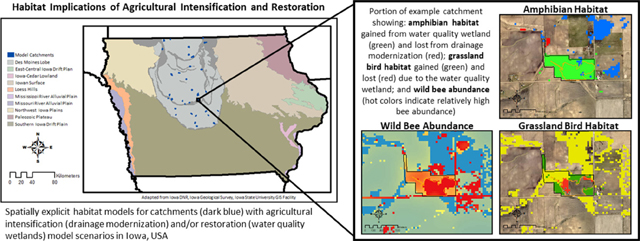
Given widespread biodiversity declines, a growing global human population, and demands to improve water quality, there is an immediate need to explore land management solutions that support multiple ecosystem services. Agricultural water quality wetlands designed to provide both water quality benefits and wetland and grassland habitat are an emerging restoration solution that may reverse habitat declines in intensive agricultural areas. Installation of water quality wetlands in the Upper Midwest, USA, when considered alongside the repair and modification of aging agricultural tile drainage infrastructure, is a likely scenario that may mitigate nutrient pollution exported from agricultural systems and improve crop yields. The capacity of water quality wetlands to provide habitat within the wetland pool and the surrounding grassland is not well-studied, particularly with respect to potential habitat changes resulting from drainage infrastructure upgrades. For the current study, we produced spatially explicit models of 37 catchments distributed throughout an important region for agriculture and biodiversity, the Des Moines Lobe of Iowa. Four scenarios were considered - with and without improved drainage and with and without water quality wetlands - to estimate the net potential habitat implications of these scenarios for amphibians, grassland birds, and wild bees. Model results indicate that drainage modification alone will likely result in moderate direct losses of suitable amphibian habitat and large declines in overall habitat quality. However, inclusion of water quality wetlands at the catchment scale may mitigate these amphibian habitat losses while also increasing grassland bird and pollinator habitat. The impacts of water quality wetlands and drainage modernization on waterfowl in the region require additional study.

Graphical Abstract

1. Introduction

Widespread grassland and wetland habitat loss, largely due to agricultural expansion, is a significant driver of ongoing, worldwide declines in biodiversity (Dahl, 1990; Davidson, 2014; Hoekstra et al., 2005; Hu et al., 2017). Given a growing global human population, there is an immediate need to explore land management solutions that can optimize crop production, improve water quality, and increase wildlife habitat. Agricultural intensification could help meet future food demands with less agricultural expansion, and coupled with targeted habitat creation or restoration could reduce or even reverse the rate of biodiversity declines related to farming (Kok et al., 2018; Tilman et al., 2011; Zedler and Kercher, 2005).

Agricultural intensification practices, such as adding or improving drainage, can increase crop production in existing agricultural areas. Agricultural drainage systems have been used throughout the world for thousands of years to remove excess soil water and prevent soil salinization in cultivated areas (Valipour et al., 2020). Presently, agricultural drainage systems including drainage ditches and subsurface drain tile installations are largely responsible for successful crop production in large portions of the U.S.A., Canada, Europe, and China. However, these drainage practices are also responsible for widespread declines in wetland and associated grassland habitat (Agency, 1996; Blann et al., 2009; Shaoli et al., 2007; Walters and Shrubsole, 2003). Further intensification through drainage modernization in some areas should increase crop yields (Evans and Fausey, 2015; Skaggs et al., 2012; Skaggs et al., 2006), but the net habitat effects of drainage modernization, and the ability of restoration solutions to counteract any resulting habitat losses, remains understudied (Mitchell et al., 2022). Herein we produce wildlife habitat models to explore the net habitat implications of combining habitat restoration/creation and agricultural drainage modernizations, with the goal of informing decision making in an important region for agricultural production and biodiversity.

The Des Moines Lobe (DML), located within the Prairie Pothole Region of North America (PPR) and spanning from central Iowa to west-central Minnesota, U.S.A., was once home to vast grasslands and depressional wetland complexes that provided habitat for grassland birds, pollinators, amphibians, and waterfowl (Gallant et al., 2011). In the years following European settlement of the region, much of the DML, particularly that portion of the region within the state of Iowa (DML-IA), was converted to row crop agriculture, facilitated by the widespread installation of subsurface and surface drainage networks. This has resulted in a nearly complete loss of native grassland and upland depressional wetland ecosystems across the DML, with much of the region now under intensive corn and soybean cultivation (Dahl, 1990; Gallant et al., 2011; Hollander, 1968; Lark et al., 2015).

Much of the existing subsurface drainage infrastructure in the DML - comprised of mains, laterals, and field tile (Fig. 1) - was installed in the early 1900s (Hollander, 1968; Kanwar et al., 1983) and is presently in disrepair or is undersized for current drainage needs (Helmers et al., 2009; Hollander, 1968; Kanwar et al., 1983). Currently, efforts are underway to repair and/or upgrade these systems to improve their drainage capacities. These anticipated repairs and upgrades may reduce the duration and extent of surface water ponding in perennially low yield farmed depressions. Reducing depressional ponding may increase crop yields (Evans and Fausey, 2015; Skaggs et al., 2012; Skaggs et al., 2006), but might also negatively affect amphibian and waterfowl habitat (Balas et al., 2012; Ballard et al., 2021; Cowardin et al., 1995; Swanson et al., 2019). However, these effects have not been adequately explored (Mitchell et al., 2022).

Fig. 1.

Diagram of a catchment indicating subsurface drainage district mains and laterals, cropped depressions, and the location of a water quality wetland positioned to capture a large portion of the flows from the catchment. Excess soil water enters field drainage tiles (not shown) before entering the drainage district main and lateral tiles and ultimately exiting the catchment at the outlet (Ditch/Waterway). Adapted from Mitchell et al. (2022).

Wetlands designed to provide both habitat and water quality benefits are an emerging restoration solution and are especially well suited to intercept and reduce nutrient loads from agricultural tile drainage networks (Crumpton et al., 2020). In recent years, water quality wetlands have been restored or developed below the outlets of local subsurface drainage districts throughout the DML-IA to both reduce nitrogen exports from artificially drained farmed catchments (Crumpton, 2001; Crumpton et al., 2020; Kalcic et al., 2018; O’Geen et al., 2010; Tomer et al., 2013) and increase wetland and grassland habitat. These wetlands, if constructed below a small catchment (e.g., 120 to 1620 ha) that has upgraded its tile mains and laterals, may be able to offset wetland habitat losses in depressional systems resulting from drainage modernization. While the water quality benefits of these restoration efforts are well established (Crumpton, 2001; Crumpton et al., 2020; Kalcic et al., 2018; O’Geen et al., 2010; Tomer et al., 2013), their ability to provide wildlife habitat is not. In addition, only a handful of studies (reviewed in Mitchell et al., 2022) have evaluated the habitat quality of cropped depressions and restored/created wetlands in the region or have explored their potential to provide additional habitat for grassland species and pollinators within the habitat buffers that typically surround restored/created wetlands. Understanding the net habitat benefits of coupling wetland restoration to drainage modernization is increasingly critical as stakeholders upgrade aging drainage infrastructure to improve crop yields (Mitchell et al., 2022).

In this study, we evaluated the net habitat implications of habitat restoration and anticipated agricultural intensification by producing spatially explicit wildlife habitat models of 37 catchments distributed throughout the DML-IA for scenarios with and without water quality wetlands and with and without drainage modernization. Model results were used to evaluate the potential effects of these landscape management alternatives on net habitat quality for amphibians, grassland birds, and wild bees.

2. Methods

2.1. Study area

The DML-IA (Fig. 2) is a glaciated sub-region of the larger DML that was dominated by grassland habitat and numerous prairie pothole wetlands prior to agricultural expansion (Dahl, 1990; Gallant et al., 2011). Presently, almost 80% of the DML-IA is under intensive row-crop agriculture (Green et al., 2019), with more than 173,000 drained depressions occurring in the region that vary in size and water storage capacity (McDeid et al., 2019). However, the region still provides habitat and resources for waterfowl (Ballard et al., 2021; Lagrange and Dinsmore, 1989; Murphy and Dinsmore, 2018) while supporting remnant populations of amphibians (Balas et al., 2012; Swanson et al., 2019), grassland birds (Sauer et al., 2013; Shaffer et al., 2019), and wild bees (Harmon-Threatt and Hendrix, 2015; Hendrix et al., 2010).

Fig. 2.

Model catchment locations (dark blue) within the Des Moines Lobe of Iowa (DML-IA; light blue). Grey polygons indicate the location of glacial moraines within the DML-IA. Note that some model catchments are directly adjacent to one another and appear as one catchment at this scale. Adapted from the Iowa – Landforms Regions and Features layer produced by Iowa DNR, Iowa Geological Survey, and the Iowa State University GIS Facility.

Subsurface drainage systems installed in the DML-IA in the mid-1800s and early 1900s were made of ceramic, called drainage “tiles”, and were laid end to end to drain fields. These old ceramic tiles and newer perforated piping, generally referred to as field tiles, commonly connect to larger diameter pipes called laterals and mains (Fig. 1). Field tiles are replaced, upgraded, or expanded upon as needed, but most of the original drainage system mains and laterals installed in the early 1900s are still in use throughout Iowa (Fig. 1; Helmers et al., 2009; Hollander, 1968; Kanwar et al., 1983). It is expected that drainage systems throughout the DML-IA will be replaced or modified in the coming decades to support ongoing and increased agricultural production (Helmers et al., 2009; Kanwar et al., 1983).

2.2. Model locations

Thirty-seven catchments located throughout the DML-IA were selected for model assessment and analysis (Fig. 2). Sites were selected within each of the region’s glacial advances (the Algona, Altamont, and Bemis advances), and were chosen to encompass a range of water quality wetland-to-catchment area ratios. A depressional volumetric storage layer (McDeid et al., 2019) was also used to locate catchments representing a range of potential depressional water storage capacities.

All model locations were representative of existing Iowa Conservation Reserve Enhancement Program (CREP) water quality wetlands (Iowa Department of Agriculture and Land Stewardship (IDALS), personal communication). Specifically, catchment areas ranged between 129 and 1296 ha (319–3203 acres), wetland-to-catchment area ratios between 0.4 and 6.4%, and deep water (>0.9 m) comprised less than 25% of respective pool areas (Table 1). Each water quality wetland was located at the drainage system outlet and encompassed by a grassland habitat buffer representing the terrestrial portion of the conservation easement that ranged from 0.5 to 6.1 times the respective wetland pool area (Table 1). All model catchments were heavily farmed, with an average of 87% and a minimum of 50% corn and soybean coverage in 2019 (Table 1).

Table 1.

Model catchment details. WQ = Water Quality.

Catchment ID	County	Catchment area (ha)	Easement area (ha)	WQ wetland area (ha)	WQ wetland: catchment area (%)	Non-depressional corn/soy (%)	Depressional corn/soy (%)	Total depressional area (%)	Existing wetland area (%)
1	Emmet	322	7	3	0.9	82	9	9	0.6
2	Emmet	287	17	3	0.9	65	19	20	3.6
3	Emmet	250	16	4	1.7	83	3	4	0.9
4	Emmet	498	22	9	1.7	60	0	1	6.7
5	Emmet	184	15	6	3.4	86	3	3	2.1
6	Hancock/Kossuth	1144	16	4	0.4	79	9	9	1.2
7	Kossuth	664	12	8	1.2	76	16	17	2.1
8	Kossuth	732	18	6	0.8	79	14	15	0.5
9	Winnebago	448	11	6	1.3	80	5	5	3.6
10	Winnebago	527	40	13	2.5	72	17	17	2.8
11	Winnebago	242	8	3	1.1	77	2	3	4.2
12	Pocahontas	945	42	7	0.7	84	11	11	0.5
13	Calhoun	651	24	8	1.2	87	8	8	0.5
14	Calhoun	233	9	2	0.9	87	10	10	0.2
15	Humboldt	608	12	3	0.5	81	5	5	2.0
16	Humboldt	432	12	2	0.4	94	2	2	0.8
17	Webster	560	11	2	0.4	83	13	13	0.1
18	Webster	372	11	3	0.7	86	8	8	0.6
19	Wright	560	42	18	3.2	81	6	6	5.0
20	Hamilton	1219	35	15	1.2	75	16	17	0.5
21	Hamilton	388	20	10	2.6	84	3	3	5.8
22	Greene	290	13	4	1.5	92	1	1	0.1
23	Greene	284	15	5	1.6	75	0	0	1.4
24	Greene	281	6	1	0.5	84	8	8	0.4
25	Greene	407	11	3	0.7	90	5	5	0.4
26	Greene/Calhoun	854	18	7	0.8	91	3	3	0.9
27	Boone/Hamilton	1296	26	11	0.9	62	4	4	4.4
28	Boone	328	7	2	0.6	87	8	8	0.5
29	Boone	260	17	4	1.7	93	3	3	0.4
30	Boone	129	25	8	6.4	87	8	8	0.6
31	Story	349	15	4	1.1	91	2	2	0.5
32	Story	531	14	7	1.4	81	10	10	0.7
33	Dallas	274	8	2	0.8	51	1	2	1.7
34	Dallas	593	12	3	0.5	61	5	6	1.2
35	Dallas	508	23	7	1.4	72	8	8	0.4
36	Polk	936	18	7	0.8	85	1	1	0.6
37	Polk	241	9	2	1.0	88	4	4	0.2

Geographic Information System software (ArcGIS Pro 2.8; Esri, Redlands, CA, USA) was used to visually identify and assess potential water quality wetland locations and to delineate pool and catchment boundaries to ensure criteria representative of existing wetland conservation program sites. Catchment and water quality wetland pool boundaries were delineated using three-meter resolution lidar-derived contours with 0.6 m (two-foot) elevation intervals obtained from the State of Iowa (https://ortho.gis.iastate.edu/arcgis/services/ortho/lidar_dem_3m/ImageServer/WMSServer). Conservation easements were delineated using standard CREP practices by creating straight-line boundaries around each water quality wetland, which at a minimum included the surrounding areas within 1.2 m of elevation above the normal pool elevation.

2.3. InVEST habitat quality and crop pollination models

The US EPA EcoService Models Library (ESML; https://esml.epa.gov/), a searchable database of ecological models for estimating the production of ecosystem goods and services (Newcomer-Johnson et al., 2019), was used for selection of the Integrated Valuation of Ecosystem Services and Tradeoffs (InVEST; Natural Capital Project) Habitat Quality (Sharp et al., 2016) and Crop Pollination models (Sharp et al., 2016). The InVEST software suite (version 3.9.0) is a collection of spatially explicit models. The Habitat Quality and Crop Pollination models have been used extensively throughout the world, including in the DML-IA to study amphibian habitat (Mushet et al., 2014; Mushet and Roth, 2020), grassland birds (Mushet and Roth, 2020; Shaffer et al., 2019), and wild bees (Koh et al., 2016).

Potential habitat or wild bee pollinator abundance in the InVEST Habitat Quality and Crop Pollination models are identified by developing spatial layers that include information about land use and land cover (Fig. 3; refer to Section 2.4). In the Habitat Quality model, potential habitat is degraded by “threats”, broadly defined as environmental factors that have the potential to disrupt habitat quality (Sharp et al., 2016). Threats could include short hydroperiods, nearby agricultural production, or other features.

Fig. 3.

Model inputs, intermediate steps, and outputs for the InVEST habitat quality model (left) and crop pollination model (right).

Habitat quality in potential habitat locations is a numerical index calculated based on the relative habitat suitability of a given LULC, the proximity of threats, their relative impact on habitat quality, and the relative sensitivity of a habitat type to a specific threat (Fig. 3; Sharp et al., 2016). The total amount of habitat quality degradation that an area experiences from threats is additive and used to calculate habitat quality using a half-saturation function and a user specified half-saturation constant.. For a given grid cell $x$ in land use type $j$, the habitat quality index $Q_{xj}$ is given by the following equation:

$${\mathrm{Q}}_{\mathrm{x}\mathrm{j}}={\mathrm{H}}_{\mathrm{j}}\left(1-\left(\frac{{\mathrm{D}}_{\mathrm{x}\mathrm{j}}^{\mathrm{z}}}{{\mathrm{D}}_{\mathrm{x}\mathrm{j}}^{\mathrm{z}}+{\mathrm{k}}^{\mathrm{z}}}\right)\right)$$

where $H_j$ is the habitat suitability of land use type $j,D_{xj}$ is the total threat level in grid cell $x$ with land use type $j$ and influenced by the proximity of threats and the relative sensitivity of land use type $j$ to these threats, $k$ is the half saturation constant, and $\text{z}$ is a scaling constant that is set to a value of 2.5 (Sharp et al., 2016). A value of 0.5, after Mushet and Roth (2020), was used in all Habitat Quality model runs for $k$. Consult Sections 2.5 and 2.6, and Sharp et al. (2016) for more information about the InVEST Habitat Quality model calculations.

The Habitat Quality model was used to calculate habitat quality and a threshold habitat quality value was applied to classify areas as suitable amphibian or grassland bird habitat (Fig. 3; refer to Sections 2.5 and 2.6, respectively for more information) for the scenarios with and without water quality wetlands and with and without drainage modernizations. For all Habitat Quality model runs, the modeled area extended to catchment boundaries plus the maximum threat distance included in the model in all directions. This extended assessment area ensures the effects of the surrounding land use, and the effects of land management scenarios on habitat outside of the catchment boundaries, are accounted for.

The InVEST Crop Pollination model (Section 2.7; Sharp et al., 2016), after Lonsdorf et al. (2009), was used to identify areas with suitable floral resources and nearby nesting sites to support wild bee pollinators based on land cover layers for the four scenarios (Fig. 3). The model calculates a relative bee abundance for each species in each season modeled, where relative bee abundance, $PA$, for species $s$ in cell $x$ in season $j$ is:

$$PA\left(x,s,j\right)=\left(\frac{RA\left(l\left(x\right),j\right)fa\left(s,j\right)}{FR\left(x,s\right)}\right)\frac{{\text{Σ}}_{x^{\text{'}}\in X}PS\left(x^{\text{'}},s\right)\text{exp}\left(-D\left(x,x^{\text{'}}\right)/\alpha s\right)}{\text{exp}\left(-D\left(x,x^{\text{'}}\right)/\alpha s\right)}$$

where $RA\left(l\right(x),j)$ is the relative abundance of floral resources for landcover $l$ in cell $x$ in season $j,fa(s,j)$ is the relative foraging activity for species s in season $j,FR(x,s)$ is the accessible floral resources index in cell $x$ for species $s$, $PS$ ($x^{\text{'}},\mathrm{s}$) is the pollinator supply index at pixel $x^{\text{'}}$ for species s and based on available nesting sites in the cell and floral resources in surrounding cells, $D\left(x,x^{\text{'}}\right)$ is the distance between cells $x$ and $x^{\text{'}}$, and $\alpha s$ is the foraging distance for species $s$ (Sharp et al., 2016). Consult Section 2.7 and Sharp et al. (2016) for more information regarding model calculations. Similar to Habitat Quality model runs, the modeled area extended to catchment boundaries plus the maximum bee species flight distance included in the model in all directions to account for interactions between the catchment and its surroundings.

2.4. Scenario land cover layers

Land use and land cover (LULC) data for the baseline scenario (e.g., Fig. 4A) was obtained from the 2019 National Agricultural Statistics Survey (NASS) Cropland Data Layer (CDL; 30 by 30 m resolution; U.S. Department of Agriculture National Agricultural Statistics Service, Cropland Data Layer. Accessed August 18, 2021. https://www.nass.usda.gov/Research_and_Science/Cropland/). This LULC layer was overlaid with a depressional storage layer and the National Wetlands Inventory (NWI; U.S. Fish and Wildlife Service, National Wetlands Inventory; Accessed August 8, 2020. https://www.fws.gov/wetlands/) to identify drained depressions and existing wetlands not identified in the NASS CDL. Drained depressions throughout the DML-IA were identified and delineated by McDeid et al. (2019) and represent depressional areas assumed to be drained because they reside within cropland and have hydric soils. Drained depressions were given unique LULC codes in the InVEST habitat quality models (e.g., Fig. 4A). Drained depressional LULC classes were based on the majority 2019 NASS CDL LULC within their bounds and were assessed as potential amphibian habitat. For example, depressional corn (e.g., Fig. 4A) corresponded to areas identified as corn that could serve as amphibian habitat under the right conditions. However, drained depressional locations were assumed to have short hydroperiods akin to temporary wetland systems and were also added to the short hydroperiod threat map. Drained depressional areas were therefore potential habitat for amphibians in our model inputs, but during model runs habitat quality was degraded by the short hydroperiod threat and any other additional location-specific threats. Existing wetlands identified in the NWI 2019 and NASS 2019 CDL layers were overlaid on drained depressions so that existing wetland habitats with a variety of hydroperiods could also be located within the drained depressional systems (e.g., Fig. 4A). Portions of drained depressional areas with extended hydroperiods were therefore distinguished from areas with short hydroperiods, and habitat in these areas was not degraded in model runs by the short hydroperiod threat like other drained depressional areas.

Fig. 4.

Land use and land cover designations for the four model scenarios (A) baseline; B) drainage modernization; C) water quality wetland; and D) drainage modernization and water quality wetland) in an example catchment. The catchment is delineated by the white outline. Corn, soy, and grassland depressional areas are indicated using a different shade of their respective land cover class colors. Modeled drainage modernizations only influence drained depressions within model catchment boundaries. LI = low intensity; MI = medium intensity; HI = high intensity; Herb. = herbaceous; Hab. = ; depress. Grass. = depressional grassland; WQ = water quality.

In this study, we used a worst-case scenario approach and assumed that drainage modernizations would result in the complete loss of any potential wetland habitat occurring within drained depressional areas within modeled catchments. Therefore, drained depressional areas were converted in the model for these scenarios to the corresponding majority land cover from the 2019 NASS CDL (e.g., Fig. 4B and D). For example, the aforementioned depressional corn areas in the baseline scenario were converted to non-depressional corn in the improved drainage scenarios. Any existing wetlands (i.e., NASS or NWI wetlands) located within drained depressions were also converted to the majority land cover of the depressional area in the 2019 NASS CDL (e.g., Fig. 4B and D), making them unsuitable as amphibian habitat.

In the water quality wetland scenarios, the baseline land cover layer was overlaid with modeled water quality wetlands within modeled conservation easements (e.g., Fig. 4C). Modeled water quality wetland and surrounding habitat buffer locations represented potential sites for the addition of water quality wetlands, as described previously, and were not already present on the landscape in the modeled locations. The addition of water quality wetlands and grassland habitat buffers therefore replaced present LULC classifications in these locations. Water quality wetlands were classified as semi-permanent wetland systems in our InVEST habitat quality models, with the surrounding conservation easement protecting any amphibian, grassland bird, or wild bee habitat. Water quality wetlands installed in Iowa and other regions are commonly surrounded by a habitat buffer extending to the conservation easement boundary that is commonly planted with a mixture of native grasses and wildflowers. The habitat buffer can range in size depending on topography, landownership, soil types, infrastructure, or other factors. Presently, the average buffer ratio in Iowa is approximately 3.5 ha for each water quality wetland pool hectare (IDALS, personal communication). This habitat buffer was classified as potential grassland bird habitat in the model, with the portions of the buffer within 160 m of the wetland also serving as potential amphibian habitat (Mushet et al., 2014). For this study, we assumed the habitat buffers surrounding water quality wetlands were established prairie restorations and therefore able to support relevant grassland bird and wild bee populations. However, the restoration of native prairie vegetation in the region can take several years to decades to reach the diversity levels observed in remnant sites in the region of interest (Carter and Blair, 2012).

2.5. Amphibian habitat InVEST model

For amphibian models, all wetlands served as potential habitat as did all land within a 160 m buffer emanating in all directions from those wetland boundaries unless it was classified as cropland (Mushet and Roth, 2020). Except for drained depressional lands and water quality wetlands, habitat and threat sensitivity values were obtained from Mushet et al. (2014; Suppl. Tables 1 and 2). Drained depressions were set to the same habitat and threat susceptibility factors as temporary wetlands in Mushet et al. (2014; Suppl. Table 2). Water quality wetlands were set to the same habitat and threat susceptibility factors as semi-permanent wetlands in Mushet et al. (2014; Suppl. Table 2). Threat weights and the distances over which they act were set to the same values as in Mushet et al. (2014; Suppl. Table 1). Threats for amphibian habitat included wetland permanence (“Lake” threat for permanent systems and “Hydro” threat for temporary systems with a short hydroperiod), proximity to cropland (“Crop” threat), and habitat isolation (“Iso” threat; Suppl. Table 1). Permanent systems can harbor fish which will decrease amphibian habitat quality, while temporary systems may dry out and become less suitable for amphibians. Therefore, semipermanent wetlands were not degraded by the “Lake” or “Hydro” threats. A wetland was considered isolated if there was no other potential amphibian habitat within a radius of 500 m. Other threats may impact amphibian habitat quality in the region, but the chosen threats were previously identified as the major factors affecting amphibians in the region of interest (Mushet et al., 2012). An evaluation area extending from the border of all modeled catchments to a distance of 1.0 km, representing the maximum threat distance, was used for all scenarios.

The threshold habitat quality score of 0.8 was established by Mushet et al. (2014) for suitable amphibian habitat in wetlands in the DML, with habitat quality values greater than or equal to this value deemed as suitable amphibian habitat. This 0.8 threshold was tested on three existing water quality wetland sites within and up to 9 km outside of the DML-IA boundary. These sites were previously found to serve as habitat for Leopard Frogs (Lithobates pipiens), American Toads (Anaxyrus americanus), and Boreal Chorus Frogs (Pseudacris maculata) by Swanson et al. (2019). Gray treefrogs (Hyla spp.) were also present at two of the three sites. Mushet and Roth’s (2020) threshold of 0.8 was found to be too restrictive, as the lowest maximum habitat quality among the three sites with documented amphibian presence was 0.6, with gray treefrogs and all other species present at this site. Therefore, in our analyses we used the 0.6 threshold, but it should be noted that this value, being the maximum value at the site with the lowest quality scores, is still likely a conservative cutoff. A less conservative threshold of 0.4 was also evaluated in the sensitivity analysis.

We performed a sensitivity analysis to explore the potential implications of the four scenarios on amphibian habitat. We tested the effects on habitat suitability of reducing threat weights, habitat sensitivity values to threats, and habitat suitability thresholds using the amphibian model to assess a range of possible outcomes for amphibian habitat in the four scenarios.

2.6. Grassland bird habitat

Potential habitat values, threat weights, and threat sensitivity values were obtained from and validated by Shaffer et al. (2019; Suppl. Tables 3 and 4). Models considered all grassland and several types of small grain to serve as potential habitat, regardless of whether they were in depressional areas. Drainage modernization was therefore expected to have minimal effects on grassland bird habitat. Small grain habitat (e.g., rye, wheat, oats; see Supplemental Table 4) was classified as less valuable habitat than grasslands and was also included as cropland in the crop threat layer (Shaffer et al., 2019). In scenarios involving the addition of water quality wetlands, areas within the conservation easement but outside of the water quality wetland that serve as habitat buffers for the water quality wetland were considered potential grassland bird habitat and classified with the same habitat value and threat sensitivity values as grasslands in Shaffer et al. (2019; Suppl. Table 4). The water quality wetland itself, however, was not considered potential habitat. Threat layers included proximity to cropland as well as to roads, urban areas, and woodlands (Mushet and Roth, 2020; Suppl. Table 3). Scenario land cover layers used for the amphibian models were modified for grassland bird models by overlaying roads (Tiger/Line city census data; U.S. Census Bureau; Accessed November 4, 2020. www.census.gov/geographies/mapping-files/time-series/geo/tiger-line-file.2019.html). The habitat quality threshold of 0.3 established and validated by Shaffer et al. (2019) was used to determine suitable grassland bird habitat, with areas exhibiting habitat quality scores equal to or greater than this value classified as suitable habitat. An evaluation area extending from the border of all modeled catchments to a distance of 1.6 km, representing the maximum threat distance, was used for all scenarios.

2.7. Pollinator resources

The InVEST Pollination model (Sharp et al., 2016) was used to assess the availability of resources for wild bees for the four model scenarios in the region. Wild bees were chosen because, together with European honeybees, they represent some of the most important pollinators for crops and native plants (Council, 2007; Winfree et al., 2008). We modeled bee species with documented presence in Iowa’s remnant native prairies (Harmon-Threatt and Hendrix, 2015) that have also previously been assessed using the Lonsdorf et al. (2009) wild bee model that forms the basis for the InVEST pollination model used in this study. The European honeybee (Apis mellifera) was also modeled because of its importance in providing pollination benefits (Council, 2007). Modeled bees were therefore widespread bee species that range throughout the Midwestern and Eastern United States. However, the modeled groups can serve as proxies for other bee species and pollinator groups as the modeled wild bee species represent a range of nesting habitat types (stem, cavity, ground, and wood nesting species included) and flight ranges (ranging from 35 m to 1515 m; Lonsdorf et al., 2009; Suppl. Table 5).

The InVEST pollination model calculates a pollinator abundance index for each species or group based on parameters for nesting requirements, seasonal activity, and flight ranges for each species or group (Fig. 3). These parameters are analyzed together with a LULC map and corresponding estimates of floral and nesting resources for each LULC type (Sharp et al., 2016). Floral resources represent the relative floral resources provided by each LULC class in each modeled season. Nesting resources represent the relative availability of stem, cavity, ground, and wood nesting for each LULC (Sharp et al., 2016).

We used the amphibian land use scenario maps described earlier for our wild bee pollinator model runs. Estimates of relative floral resource availability for each LULC type in spring, summer, and fall were based on expert opinion for the Great Plains (Mushet and Scherff, 2016; Suppl. Table 6). Relative nesting resources for each LULC type were based on the mean of expert opinion estimates for the United States obtained from Koh et al. (2016). Depressional land cover types were set to the same floral and nesting resources as their corresponding non-depressional land-cover type (Suppl. Table 6). This approach results in no change in the floral or nesting resources for a depressional area with drainage modernization; therefore, drainage modernization could not affect wild bee abundance except in cases where existing wetlands (i.e., NWI and NASS CDL wetlands) occurred within depressions. Nesting requirements, seasonal activity, and flight ranges for each bee species were obtained from Lonsdorf et al. (2009). Where multiple species were included from a genus, they were grouped, and means of seasonal activity indices and flight ranges were used for model inputs (Suppl. Table 5). The following species were modeled: Apis mellifera (Western honey bee), Agapostemon virescens (bicolored striped-sweat bee), Augochlorella aurata (golden green-sweat bee), Augochloropsis metallica (metallic epauletted-sweat bee), Bombus fervidus (golden northern bumble bee), B. bimaculatus (two-spotted bumble bee), Ceratina dupla (doubled ceratina), Halictus confusus (confusing furrow bee), H. ligatus (ligated furrow bee), Hylaeus affinis (Eastern masked bee), Hyl. Modestus (modest masked bee), Lasioglossum admirandum (admirable sweat bee), L. pilosum (hairy metallic-sweat bee), L. rohweri (no common name), L. coriaceum (leathery sweat bee), and Melissodes bimaculata (two-spotted longhorn bee).

3. Results

3.1. Amphibian habitat

Modeled catchments included 1484 ha of drained depressional areas, with 39 ha of that identified as existing wetlands in the NWI and 2019 NASS CDL layers. 2019 was the twelfth wettest year on record for Iowa, with counties throughout the DML-IA experiencing precipitation levels well above average (IDALS, 2019).

The baseline scenario provided 981 ha of modeled suitable amphibian habitat within and extending 1 km from modeled catchment boundaries (Table 2), amounting to 1.4% of the modeled area. The majority (89%) of this suitable habitat was located outside the 37 modeled catchment boundaries. Only 3.6% of the land occurring within depressions served as suitable amphibian habitat in the baseline scenario, due largely to the presence of existing wetlands (as identified in the NWI and NASS CDL layers) occurring within depressions. Using the more conservative threshold value of 0.8 for suitable amphibian habitat developed by Mushet et al. (2014), only 0.5% of the evaluated area was found to serve as suitable amphibian habitat in the baseline scenario (Table 3).

Table 2.

InVEST model results for the four scenarios. Assessment scales differ by ecosystem service because models operate over different scales. Scales refer to the area within and extending 0–1.6 km outwards from all modeled catchment boundaries. Green cells indicate gains in habitat or habitat quality, orange cells indicate losses, and grey cells indicate minimal (<1%) change.

Habitat Metric	Baseline Scenario (ha)	Drainage Modernization (Change from Baseline)	Water Quality Wetland (Change from Baseline)	Drainage Modernization and Water Quality Wetland (Change from Baseline)
Amphibian Habitat (ha) Within 1 km	981	−3%	+25%	+22%
Amphibian Habitat Total Quality Score Within 1 km	32,002	−21%	+12%	−10%
Bee Total Pollinator Abundance Score Within Watershed	5,382	−0.4%	+10%	+10%
Grassland Bird Habitat (ha) Within 1.6 km	7,029	+0.04%	+5%	+5%
Grassland Bird Total Quality Score Within 1.6 km	79,036	+0.04%	+5%	+5%

Table 3.

Sensitivity analysis results (area of amphibian habitat within 1 km of catchment boundaries) for InVEST amphibian habitat suitability models with varying threat weights, habitat sensitivity values, and habitat suitability thresholds. The base model, with a habitat suitability threshold of 0.6 and threat weights and habitat sensitivity settings after Mushet et al., 2014, was the primary amphibian model referenced in the present study. CT = crop threat; LT = Lake threat; HT = Short hydroperiod threat; IT = Isolation threat; CS = Habitat sensitivity to crop threat; LS = Habitat sensitivity to lake threat; HS = Habitat sensitivity to short hydroperiod threat; IS = Habitat sensitivity to isolation threat. Areas are in hectares.

			Baseline Scenario Amphibian Habitat within 1km (ha)			Drainage Modernization Scenario Amphibian Habitat within 1km (ha)			Water Quality Wetland Scenario Habitat within 1km (ha)			Drainage Modernization and WQ Wetlands Scenario Habitat within 1km (ha)
Total Area Within 1km of Catchment Boundaries			67,892			67,892			67,892			67,892
All Potential Habitat, Including Depressions			6,529			5,052			7,061			5,589
All Potential Habitat, Not Including Depressions			1,835			1,803			2,371			2,340
Habitat Suitability Threshold			≥ 0.4	≥ 0.6	≥ 0.8	≥ 0.4	≥ 0.6	≥ 0.8	≥ 0.4	≥ 0.6	≥ 0.8	≥ 0.4	≥ 0.6	≥ 0.8
	1	Base Model, After Mushet et al. (2014) CT=0.6, LT=0.2, HT=0.1, IT=0.1; CS=1, LS=0.5, HS=0.5, IS=1	3,860	981	361	3,059	955	359	4,479	1,222	383	3,620	1,197	381
Habitat Suitability Models	2	Balanced Threat Weights CT=0.25, LT=0.25, HT=0.25, IT=0.25; Habitat Sensitivities as in Base Model	6,055	6,055	3,291	4,579	4,579	2,696	6,600	6,600	3,868	5,127	5,127	3,248
	3	Reduced Crop Threat Weight CT=0.4, LT=0.2, HT=0.2, IT=0.2; Habitat Sensitivities as in Base Model	6,055	3,809	908	4,579	3,052	896	6,600	4,403	1,173	5,127	3,604	1,161
	4	Reduced Wetland & Depressional Habitat Sensitivity to Crop and Isolation Threats Threat Weights as in Base Model; CS=0.5, LS=0.5, HS=0.5, IS=0.5	6,055	6,055	2,306	4,579	4,579	2,025	6,600	6,600	2,931	5,127	5,127	2,590
	5	Increased Depressional Habitat Sensitivity to Short Hydroperiod Threat Threat Weights and Sensitivity as in Base Model; Depressional: CS=1, LS=0.5, HS=1, IS=1	2,773	945	355	2,342	928	354	3,399	1,188	377	2,902	1,170	375
	6	Reduced Wetland & Depressional Habitat Sensitivity to All Threats Threat Weights as in Base Model; CS=0.25, LS=0.25, HS=0.25, IS=0.25	6,055	6,055	6,055	4,579	4,579	4,579	6,600	6,600	6,600	5,127	5,127	5,127

CT = Crop threat.

LT = Lake threat.

HT = Short hydroperiod threat.

IT = Isolation threat.

CS = Sensitivity of habitat to crop threat.

LS = Sensitivity of habitat to lake threat.

HS = Sensitivity of habitat to short hydroperiod threat.

IS = Sensitivity of habitat to isolation threat.

Drainage modernization, represented in our models as the total loss of potential habitat within drained depressions in the catchment, resulted in a 2.6% decline (26 ha loss) in suitable amphibian habitat relative to the baseline within 1 km of the catchment (Table 2; e.g., Fig. 5). This loss represents all suitable amphibian habitat occurring within drained landscape depressions within our model catchments in the baseline scenario. However, the total amphibian habitat quality score declined 21.2% due to modeled drainage modernization (Table 2), including the degradation of potential amphibian depressional habitat not classified as suitable amphibian habitat using the habitat suitability threshold of 0.6 in the baseline scenario.

Fig. 5.

Suitable amphibian habitat in four example model catchments (white border). Water quality wetlands (orange border) and surrounding conservation easements (black border) are shown, together with suitable habitat gained from the addition of the modeled water quality wetland (green areas), lost suitable habitat due to drainage modernization (red areas), and suitable amphibian habitat in all scenarios (blue areas). Panel D represents stacked water quality wetlands across two catchments. Basemap imagery from United States Department of Agriculture’s National Agriculture Imagery Program (NAIP).

Adding a water quality wetland to all 37 catchments in the model resulted in the addition of 241 ha of suitable amphibian habitat, with 94% of the habitat gains occurring within the modeled catchments, and an 11.8% improvement in the total habitat quality score relative to the baseline (Table 2; e.g., Fig. 5). This scenario consisted of the addition of 213 ha of water quality wetlands, with an additional 635 ha of conservation easement. For each hectare of water quality wetland added, 1.1 ha of amphibian habitat were added. For each hectare of total conservation easement added, including the water quality wetlands, 0.4 ha of amphibian habitat were gained. However, only 17 of the 37 modeled conservation easements provided suitable amphibian habitat within their easement borders. The other 20 wetland-conservation easement additions failed to directly provide any suitable habitat due to degradation of these potential habitats by nearby cropland and isolation from other wetland habitat. The majority (85%) of the additional suitable amphibian habitat gained from constructing water quality wetlands occurred within the wetland or in the surrounding habitat buffer. The other 15% of the gain in suitable amphibian habitat relative to the baseline scenario occurred outside the conservation easements (e.g., Fig. 5B) due to buffering of the surrounding habitat from nearby cropland and reductions in habitat isolation.

Pairing modeled drainage modernizations with water quality wetlands resulted in an increase of 217 ha of suitable amphibian habitat relative to the baseline scenario, 93% of which was located within the modeled catchment boundaries. However, overall habitat quality declined by 9.7% relative to the baseline scenario (Table 2), reflecting a widespread decrease in the habitat quality score of drained depressional areas that were not identified as suitable amphibian habitat in the baseline scenario.

Sensitivity analysis indicates that amphibian habitat suitability is highly sensitive to the habitat suitability threshold, threat weights (particularly crop threat weight), and the sensitivity of wetland and depressional zones to threats (Table 3). In all cases, much greater proportions of water quality wetlands and depressional areas were identified as suitable habitat when threat weights or habitat sensitivity values were reduced relative to the base model settings and habitat suitability threshold of 0.6. With lower threshold, weight, and habitat sensitivity values, the addition of water quality wetlands does provide substantial amphibian habitat but no longer offsets losses of suitable habitat due to drainage modernizations because more depressional areas are identified as suitable habitat in the baseline and water quality wetland scenarios (Table 3).

3.2. Grassland bird habitat

In the baseline scenario, modeled grassland bird habitat located within 1.6 km of our modeled catchments totaled 7029 ha (Table 2), or 6.7% of the assessed area, with only 13% of the habitat residing within the modeled catchment boundaries. Drainage modernizations resulted in the gain of three hectares of suitable grassland bird habitat in the assessed area, with all of it occurring within the catchment boundaries (Table 2; e.g., Fig. 6); a minimal change in habitat that is well within the margin of error of the 2019 NASS CDL layer. Grassland bird habitat quality change was also minimal, improving by less than 0.1% (Table 2; Fig. 6A). Small improvements were a result of the conversion of wetlands located in depressions with majority grassland coverage to grassland habitat when drainage was improved (e.g., Fig. 6A).

Fig. 6.

Suitable grassland bird habitat in four example model catchments (white border). Water quality wetlands (orange border) and surrounding conservation easements (black border) are shown, together with additional suitable amphibian habitat resulting from the addition of the modeled water quality wetland (green areas), lost suitable habitat due to water quality wetland installation (red areas), suitable habitat gained from drainage modernization (purple areas), and suitable amphibian habitat in all scenarios (yellow areas). Basemap imagery from United States Department of Agriculture’s National Agriculture Imagery Program (NAIP).

Regardless of modeled drainage modernizations, adding water quality wetlands and their surrounding habitat buffers to all modeled catchments resulted in the addition of 372 ha of suitable grassland bird habitat, representing a 5.3% increase (Table 2; e.g., Fig. 6) and a 5.2% improvement in habitat quality over the baseline scenario (Table 2). Most of the habitat gains (98%) took place within the catchment boundaries. For each hectare of conservation easement (including the water quality wetland and surrounding habitat buffer), 0.6 ha of suitable grassland bird habitat was gained. Since wetlands do not directly provide habitat in the grassland bird InVEST habitat quality model, just accounting for the buffer habitat (i.e., excluding water quality wetland area) within the conservation easement resulted in a gain of 0.9 ha of suitable grassland bird habitat for each hectare of buffer habitat added.

3.3. Pollinator resources

Drainage modernizations resulted in only minimal effects on modeled total wild bee abundance at the catchment scale, with a decline of 0.4% across all wild bee groups and catchments (Table 2; e.g., Fig. 7). Small declines in modeled wild bee abundance from drainage modernizations were due to the loss of existing wetlands (NWI and NASS CDL wetlands) within catchment depressions in the model, with the negative effects of these wetland losses observed mostly within catchment boundaries (92%; Table 4). Ceratina dupla, the only species of stem-nesting bee modeled (Suppl. Table 5), had the highest decline relative to the baseline when drainage was improved, with abundance declining by 1.0% at the catchment scale. All other groups had declines of 0.5% or less at the catchment scale relative to the baseline scenario (Table 4).

Fig. 7.

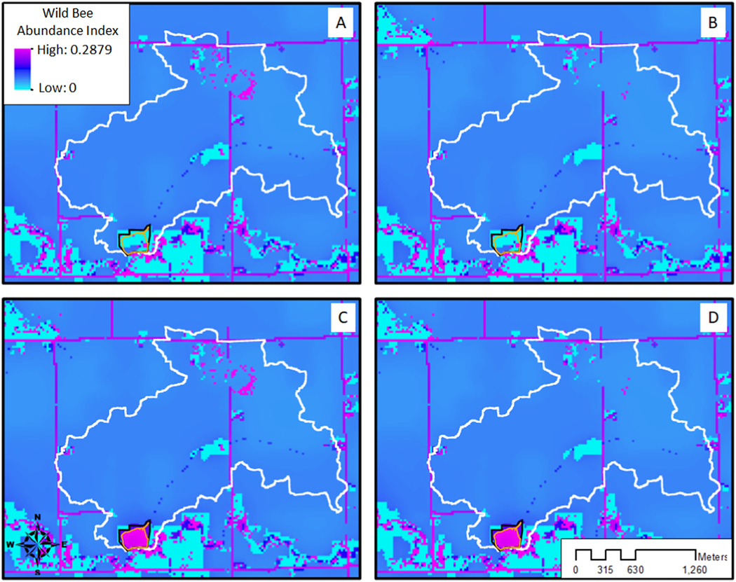
Total wild bee pollinator abundance for the A) baseline, B) drainage modernization, C) water quality wetland, and D) drainage modernization and water quality wetland scenarios for an example catchment (white border), model water quality wetland (orange border), and surrounding conservation easement (black border).

Table 4.

Wild bee abundance indices from the InVEST Pollination model for the four scenarios. Except where indicated, pollinator abundance results are for areas contained within and extending 5 km outwards from all modeled catchment boundaries. Drain. Mod. = drainage modernization; WQ = water quality.

Season		Spring				Summer				Fall				Total
Scenario		Baseline	Drain. Mod.	WQ Wetland	Drain. Mod. & WQ Wetland	Baseline	Drain. Mod.	WQ Wetland	Drain. Mod. & WQ Wetland	Baseline	Drain. Mod.	WQ Wetland	Drain. Mod. & WQ Wetland	Baseline	Drain. Mod.	WQ Wetland	Drain. Mod. & WQ Wetland
Species/Genus	Apis mellifera	1453	1452	1468	1467	6269	6268	6297	6296	593	592	599	598	8315	8313	8364	8362
	Agapostemon virescens	0	0	0	0	16514	16513	16579	16578	1383	1382	1397	1398	17898	17896	17977	17976
	Augochlorella aurata	2304	2302	2339	2338	9315	9314	9356	9356	944	943	958	958	12562	12560	12653	12651
	Augochloropsis metallica	0	0	0	0	16422	16421	16489	16488	1406	1406	1423	1422	17828	17827	17912	17910
	Bombus	1433	1432	1448	1447	6293	6292	6319	6318	587	586	593	592	8312	8310	8359	8357
	Cera tin a dupla	2032	2030	2060	2059	6752	6750	6780	6778	782	781	793	792	9565	9562	9632	9629
	Halictus	2282	2281	2313	2312	9424	9424	9466	9466	933	933	945	945	12640	12637	12724	12722
	Hylaeus	0	0	0	0	11420	11418	11437	11435	1041	1040	1049	1048	12461	12458	12486	12483
	Lasioglossum	2300	2298	2333	2331	9380	9379	9422	9421	940	940	954	953	12620	12618	12708	12706
	Melissodes bimaculata	0	0	0	0	16657	16656	16718	16717	1341	1341	1354	1353	17998	17996	18072	18070
Totals Catchment + 5km Buffer		11803	11796	11961	11953	108446	108435	108862	108852	9950	9945	10065	10061	130199	130176	130888	130866
Totals Within Catchment		343	336	488	480	4700	4691	4986	4978	340	335	444	439	5382	5362	5918	5897

Adding water quality wetlands to the modeled catchments without drainage modernizations resulted in an increase in modeled total wild bee abundance of 9.9% at the catchment scale relative to the baseline (Table 2; e.g., Fig. 7). Increases at the catchment scale represented 78% of the total modeled improvements, with additional gains occurring outside of the catchment (Table 4). Water quality wetlands particularly benefited bee species that nest in stems or the ground and have relatively small flight ranges. For example, Ceratina dupla, Augochlorella aurata, Lasioglossum spp., and Halictus spp. experienced gains in total abundance of 17.8, 16.6, 15.6, and 14.6% relative to the baseline scenario at the catchment scale, respectively. Ceratina dupla is the only stem-nesting bee modeled while Augochlorella aurata, Lasioglossum spp., and Halictus spp. nest in the ground (Suppl. Table 5; Lonsdorf et al., 2009). All other modeled species experienced lesser improvements of 9% or less, including other ground nesting bee species (Agapostemon spp., Augochloropsis metallica, and Melissodes bimaculata) which had much greater flight ranges (Table 4; Suppl. Table 5).

Drainage modernizations paired with the addition of water quality wetlands resulted in a 9.6% gain in total wild bee abundance across all modeled bee species and catchments (Table 2; e.g., Fig. 7). Increases at the catchment scale in this scenario represented 77% of the total modeled improvements (Table 4). However, modeled wild bee abundance was higher in the scenario where water quality wetlands were added but no drainage modernizations were undertaken (Table 2).

4. Discussion

In this study we took a worst-case scenario approach and assumed that drainage modernizations would result in the complete loss of any wetland habitat occurring within drained depressional areas. This approach suggests that drainage modernizations will result in moderate losses of suitable amphibian habitat and large declines in overall habitat quality. However, water quality wetlands at the catchment scale are likely to offset possible amphibian habitat losses, with the added benefit of also providing additional grassland bird habitat and pollinator resources.

Our model results suggest that water quality wetlands and their surrounding conservation buffer habitats, regardless of drainage modernizations, may be a reasonable strategy for restoring amphibian, grassland bird, and pollinator habitat to an area that has experienced drastic habitat declines over the last century. Similarly, field sampling within the DML-IA by Knutson et al. (2004), Reeves et al. (2016), and Swanson et al. (2019) indicate that water quality wetlands and agricultural ponds can indeed provide suitable habitat for several amphibian species. Additionally, our model results suggest that building water quality wetlands and associated grassland buffers may also provide suitable habitat for grassland birds and pollinators. This effect on habitat improvements by water quality wetlands might be amplified if these systems are strategically located in clusters or in close proximity to each other or another natural habitat (e.g., Fig. 5C and D).

However, our results suggest that water quality wetlands are not a panacea, as only 17 of 37 water quality-habitat buffer complexes in our model analysis provided suitable amphibian habitat; a potential concern if amphibians displaced by drainage modernizations must rely on these areas. If suitable amphibian habitat is a desired outcome, the existing habitat surrounding a potential water quality wetland site should be considered during the planning process to reduce the threat of nearby cropland and habitat isolation.

Results from the scenario with improved drainage and water quality wetlands suggest that landowners may be able to realize increased crop yields from drainage modernizations with no net loss of suitable amphibian habitat, provided a water quality wetland is developed below or within the catchment and near other wetland habitat. However, overall amphibian habitat quality remained lower than the status quo in models with improved drainage, even when water quality wetlands were added. Therefore, drainage modernizations in tile-drained, farmed catchments in the DML-IA could affect amphibian population sizes, health, and resilience, regardless of the potential habitat benefits of water quality wetlands. We believe that the potential for amphibian habitat quality reduction with drainage modernizations is an area that requires additional study.

Work is needed to assess the impacts of drainage modernization and water quality wetlands on waterfowl habitat. Waterfowl represent a diverse group, but in general they prefer relatively stable water levels and wetland connectivity (Ballard et al., 2021; Ma et al., 2010; Naugle et al., 2001) and are negatively associated with agricultural fields (Greenwood et al., 1995; Klett et al., 1988); habitat characteristics they share with many amphibians inhabiting the region (Babbitt et al., 2003; Hayes et al., 2006; Knutson et al., 2000; Mushet et al., 2014; Semlitsch, 2000; Swanson et al., 2018). If amphibian habitat also serves as waterfowl habitat in the region, water quality wetlands have the potential to increase waterfowl habitat. This assumption is supported by Otis et al. (2010) from their modeling study of the likely effect of wetland restorations on waterfowl habitat in the DML-IA, however additional work is needed to also model and assess the combined impacts of drainage modernization and water quality wetlands on waterfowl habitat in this region.

Based on our findings, we recommend that catchment-specific characteristics should be assessed prior to locating and designing wetland additions or restoration opportunities and evaluating their habitat mitigation potential. For example, we anticipate many amphibian species will benefit from wetlands that are designed or maintained as semipermanent systems, located close to other wetland habitat, and protected from the surrounding agricultural land by habitat buffers. Further, we expect that grassland birds, wild bees, and other pollinators will benefit from large conservation easements surrounding wetlands that are seeded with and maintained as grassland and wildflower communities. Our models also reinforce the potential tradeoffs between amphibian or waterfowl habitat and grassland bird habitat, particularly if wetlands replace grasslands. Larger grassland habitat buffers surrounding water quality wetlands or careful placement of water quality wetlands could minimize these tradeoffs, but at least in agriculturally dense regions this may necessitate additional reductions in productive cropland.

Other regions or landscapes may pose unique challenges or circumstances that will require modifications to the models used in this study. For example, studies investigating the potential impacts of drainage modernization on wildlife habitat in less agriculturally dense regions may wish to incorporate additional scenarios that account for the potential conversion of marginal lands within the catchment to cropland made possible by catchment-scale drainage modernizations. Additionally, in regions where surface drainage systems (e.g., drainage ditches, canals) predominate, conversion of these potential habitats and dispersal routes (e.g., Tölgyesi et al., 2022) to subsurface drainage systems with drainage modernization may have additional consequences for wildlife.

While our models suggest that water quality wetlands and their surrounding conservation easements will provide substantial habitat with the potential to offset losses from drainage modernizations, this approach has several limitations and simplifications. First, we assumed that modernization of the drainage system mains and laterals, which we anticipate will take place throughout the region in the coming years, would result in the complete loss of wetland functionality in drained depressions in the study catchments. While drainage modernizations will undoubtedly influence the hydrology of the region, this impact will vary from catchment to catchment depending on the degree of drainage modernization and catchment-specific hydrologic conditions. It is also possible that drainage modernization may influence the hydrology of other wetland habitat located outside of drained depressions, the potential effects of which were not considered here. Additionally, we did not attempt to incorporate the potential effects of temporal variability or future changes in climate (e.g., Johnson et al., 2005) on habitat. Nor did we model the influence of variability in vegetation type or abundance within conservation easements, an aspect that is likely to be a significant determinant of habitat success for wildlife (e.g., Ballard et al., 2021; Harmon-Threatt and Hendrix, 2015). Lastly, we did not attempt to quantify the crop yield benefits from drainage modernizations or potential yield losses where cropland was replaced with water quality wetlands. In total the 37 water quality wetlands and their habitat buffers replaced 251 ha of corn and 236 ha of soy, with resulting losses sure to offset some of the benefits of drainage modernizations. Continued study of these aspects, together with improved models for waterfowl habitat and additional field validation of wildlife habitat in cropped depressions and water quality wetlands in the modeled region and other landscapes, is suggested to better understand the future implications of agricultural landscape management practices on wildlife.

5. Conclusions

Without additional field validations, our modeled results should not be used to justify the expansion or modernization of agricultural drainage. However, we have demonstrated that water quality wetlands are likely to be an effective option for reestablishing amphibian habitat to the region and at least partially offsetting the direct effects of agricultural subsurface drainage modernization on amphibian habitat, provided they are located nearby existing wetland habitat. Water quality wetlands and their surrounding conservation easements are also likely to supply much needed grassland bird and pollinator habitat; however, their ability to mitigate waterfowl habitat requires further study. Water quality wetlands are therefore an important tool that may help tackle historic and ongoing habitat loss from agricultural expansion and improve downstream water quality.

HIGHLIGHTS.

• Management solutions that optimize crop yields and increase habitat are needed.

• We modeled habitat impact of drainage modernization and water quality wetlands (WQW).

• Modeled WQW and buffers provided amphibian, grassland bird, and wild bee habitat.

• Modeled WQW habitat gains mitigated modeled losses from drainage modernization.

• The impacts of drainage modernization on waterfowl require additional study.

References

- Agency EE, 1996. Human Interventions in the Hydrological Cycle. [Google Scholar]
- Babbitt KJ, Baber MJ, Tarr TL, 2003. Patterns of larval amphibian distribution along a wetland hydroperiod gradient. Can. J. Zool. 81 (9), 1539–1552. [Google Scholar]
- Balas CJ, Euliss NH, Mushet DM, 2012. Influence of conservation programs on amphibians using seasonal wetlands in the prairie pothole region. Wetlands 32 (2), 333–345. [Google Scholar]
- Ballard DC, Jones OE III, Janke AK, 2021. Factors affecting wetland use by spring migrating ducks in the southern prairie pothole region. J. Wildl. Manag 85 (7), 1490–1506. [Google Scholar]
- Blann KL, Anderson JL, Sands GR, Vondracek B, 2009. Effects of agricultural drainage on aquatic ecosystems: a review. Crit. Rev. Environ. Sci. Technol 39 (11), 909–1001. [Google Scholar]
- Carter DL, Blair JM, 2012. Recovery of native plant community characteristics on a chronosequence of restored prairies seeded into pastures in West-Central Iowa. Restor. Ecol 20 (2), 170–179. 10.1111/j.1526-100x.2010.00760.x. [DOI] [Google Scholar]
- Council NR, 2007. Committee on the Status of Pollinators in North America. Status of Pollinators in North America. National Academy Press, USA. [Google Scholar]
- Cowardin LM, Shaffer TL, Arnold PM, 1995. Evaluations of Duck Habitat and Estimation of Duck Population Sizes With a Remote-sensing-based System. vol. 2. US Department of the Interior, National Biological Service. [Google Scholar]
- Crumpton WG, 2001. Using wetlands for water quality improvement in agricultural watersheds; the importance of a watershed scale approach. Water Sci. Technol 44 (11–12), 559–564. 10.2166/wst.2001.0880. [DOI] [PubMed] [Google Scholar]
- Crumpton WG, Stenback GA, Fisher SW, Stenback JZ, Green DIS, 2020. Water quality performance of wetlands receiving nonpoint-source nitrogen loads: nitrate and total nitrogen removal efficiency and controlling factors. J. Environ. Qual 49 (3), 735–744. 10.1002/jeq2.20061. [DOI] [PubMed] [Google Scholar]
- Dahl TE, 1990. Wetlands Losses in the United States, 1780’s to 1980’s. US Department of the Interior, Fish and Wildlife Service. [Google Scholar]
- Davidson NC, 2014. How much wetland has the world lost? Long-term and recent trends in global wetland area. Mar. Freshw. Res 65 (10), 934–941. [Google Scholar]
- Evans RO, Fausey NR, 2015. Effects of inadequate drainage on crop growth and yield. In: Skaggs RW, van Schilfgaarde J (Eds.), Agronomy Monographs. American Society of Agronomy, Crop Science Society of America, Soil Science Society of America, pp. 13–54. [Google Scholar]
- Gallant AL, Sadinski W, Roth MF, Rewa CA, 2011. Changes in historical Iowa land cover as context for assessing the environmental benefits of current and future conservation efforts on agricultural lands. J. Soil Water Conserv 66 (3), 67A–77A. 10.2489/jswc.66.3.67A. [DOI] [Google Scholar]
- Green DI, McDeid SM, Crumpton WG, 2019. Runoff storage potential of drained upland depressions on the Des Moines Lobe of Iowa. JAWRA J.Am.Water Resour.Assoc. 55 (3), 543–558. [Google Scholar]
- Greenwood RJ, Sargeant AB, Johnson DH, Cowardin LM, Shaffer TL, 1995. Factors associated with duck nest success in the prairie pothole region of Canada. Wildl. Monogr 3–57. [Google Scholar]
- Harmon-Threatt AN, Hendrix SD, 2015. Prairie restorations and bees: the potential ability of seed mixes to foster native bee communities. Basic Appl.Ecol. 16 (1), 64–72. [Google Scholar]
- Hayes TB, Case P, Chui S, Chung D, Haeffele C, Haston K, Parker J, 2006. Pesticide mixtures, endocrine disruption, and amphibian declines: are we underestimating the impact? Environ. Health Perspect 114 (Suppl. 1), 40–50. [DOI] [PMC free article] [PubMed] [Google Scholar]
- Helmers MJ, Melvin S, Lemke D, 2009. Drainage Main Rehabilitation in Iowa. World Environmental and Water Resources Congress 2009. 2009/05/12/. [Google Scholar]
- Hendrix SD, Kwaiser KS, Heard SB, 2010. Bee communities (Hymenoptera: Apoidea) of small Iowa hill prairies are as diverse and rich as those of large prairie preserves. Biodivers. Conserv 19 (6), 1699–1709. [Google Scholar]
- Hoekstra JM, Boucher TM, Ricketts TH, Roberts C, 2005. Confronting a biome crisis: global disparities of habitat loss and protection. Ecol. Lett 8 (1), 23–29. [Google Scholar]
- Hollander G, 1968. Improving Old Water Management Systems in the Cornbelt. [Google Scholar]
- Hu S, Niu Z, Chen Y, Li L, Zhang H, 2017. Global wetlands: potential distribution, wetland loss, and status. Sci. Total Environ 586, 319–327. [DOI] [PubMed] [Google Scholar]
- Iowa Department of Agriculture and Land Stewardship (IDALS), 2019. Iowa Annual Weather Summary. IDALS. [Google Scholar]
- Johnson WC, Millett BV, Gilmanov T, Voldseth RA, Guntenspergen GR, Naugle DE, 2005. Vulnerability of northern prairie wetlands to climate change. Bioscience 55 (10), 863–872. [Google Scholar]
- Kalcic M, Crumpton W, Liu X, D’Ambrosio J, Ward A, Witter J, 2018. Assessment of beyond-the-field nutrient management practices for agricultural crop systems with subsurface drainage. J. Soil Water Conserv 73 (1), 62–74. 10.2489/jswc.73.1.62. [DOI] [Google Scholar]
- Kanwar RS, Johnson HP, Schult D, Fenton TE, Hickman RD, 1983. Drainage needs and returns in north-central Iowa. Trans.ASAE 26 (2), 0457–0464. 10.13031/2013.33958. [DOI] [Google Scholar]
- Klett AT, Shaffer TL, Johnson DH, 1988. Duck nest success in the prairie pothole region.J. Wildl. Manag 431–440. [Google Scholar]
- Knutson MG, Sauer JR, Olsen DA, Mossman MJ, Hemesath LM, Lannoo MJ, 2000. Landscape associations of frog and toad species in Iowa and Wisconsin, USA. J.Iowa Acad.Sci 107 (3–4), 134–145. [Google Scholar]
- Knutson MG, Richardson WB, Reineke DM, Gray BR, Parmelee JR, Weick SE, 2004. Agricultural ponds support amphibian populations. Ecol. Appl 14 (3), 669–684. [Google Scholar]
- Koh I, Lonsdorf EV, Williams NM, Brittain C, Isaacs R, Gibbs J, Ricketts TH, 2016. Modeling the status, trends, and impacts of wild bee abundance in the United States. Proc. Natl. Acad. Sci 113 (1), 140–145. [DOI] [PMC free article] [PubMed] [Google Scholar]
- Kok MT, Alkemade R, Bakkenes M, van Eerdt M, Janse J, Mandryk M, van Oorschot M, 2018. Pathways for agriculture and forestry to contribute to terrestrial biodiversity conservation: a global scenario-study. Biol. Conserv 221, 137–150. [Google Scholar]
- Lagrange TG, Dinsmore JJ, 1989. Habitat use by mallards during spring migration through Central Iowa. J. Wildl. Manag 53 (4), 1076. 10.2307/3809613. [DOI] [Google Scholar]
- Lark TJ, Salmon JM, Gibbs HK, 2015. Cropland expansion outpaces agricultural and biofuel policies in the United States. Environ. Res. Lett 10 (4), 044003. [Google Scholar]
- Lonsdorf E, Kremen C, Ricketts T, Winfree R, Williams N, Greenleaf S, 2009. Modelling pollination services across agricultural landscapes. Ann. Bot 103 (9), 1589–1600. [DOI] [PMC free article] [PubMed] [Google Scholar]
- Ma Z, Cai Y, Li B, Chen J, 2010. Managing wetland habitats for waterbirds: an international perspective. Wetlands 30 (1), 15–27. [Google Scholar]
- McDeid SM, Green DI, Crumpton WG, 2019. Morphology of drained upland depressions on the Des Moines Lobe of Iowa. Wetlands 39 (3), 587–600. [Google Scholar]
- Mitchell ME, Shifflett SD, Newcomer-Johnson T, Hodaj A, Crumpton W, Christensen J, Forshay KJ, 2022. Ecosystem services in Iowa agricultural catchments: hypotheses for scenarios with water quality wetlands and improved tile drainage. (In Press) J. Soil Water Conserv 77 (4). 10.2489/jswc.2022.00127. [DOI] [Google Scholar]
- Murphy KT, Dinsmore SJ, 2018. Waterbird use of sheetwater wetlands in Iowa’s prairie pothole region. Wetlands 38 (2), 211–219. 10.1007/s13157-015-0706-7. [DOI] [Google Scholar]
- Mushet DM, Roth CL, 2020. Modeling the supporting ecosystem services of depressional wetlands in agricultural landscapes. Wetlands 40 (5), 1061–1069. 10.1007/s13157-020-01297-2. [DOI] [Google Scholar]
- Mushet DM, Scherff EJ, 2016. The Integrated Landscape Modeling Partnership-Current Status and Future Directions (2331–1258). [Google Scholar]
- Mushet DM, Euliss NH Jr., Stockwell CA, 2012. A conceptual model to facilitate amphibian conservation in the northern Great Plains. Great Plains Res. 45–58. [Google Scholar]
- Mushet DM, Neau JL, Euliss NH Jr., 2014. Modeling effects of conservation grassland losses on amphibian habitat. Biol. Conserv 174, 93–100. [Google Scholar]
- Naugle DE, Johnson RR, Estey ME, Higgins KF, 2001. A landscape approach to conserving wetland bird habitat in the prairie pothole region of eastern South Dakota. Wetlands 21 (1), 1–17. [Google Scholar]
- Newcomer-Johnson T, Bruins R, Lomnicky G, Wilson J, Hodaj A, Maurice C, DeWitt T, 2019. EPA’s EcoService Models Library (ESML): applied use cases for a new tool for quantifying and valuing ecosystem services. Oral Presentation Presented at the Society of Environmental Toxicology and Chemistry (SETAC) North America 40th Annual Meeting, Toronto, ON, CA. [Google Scholar]
- O’Geen AT, Budd R, Gan J, Maynard JJ, Parikh SJ, Dahlgren RA, 2010. Mitigating Nonpoint Source Pollution in Agriculture With Constructed and Restored Wetlands. Advances in Agronomyvol. 108. Elsevier, pp. 1–76. [Google Scholar]
- Otis DL, Crumpton WG, Green D, Loan-Wilsey AK, McNeely RL, Kane KL, Vandever M, 2010. Assessment of Environmental Services of CREP Wetlands in Iowa and the Midwestern Corn Belt. [Google Scholar]
- Reeves RA, Pierce CL, Smalling KL, Klaver RW, Vandever MW, Battaglin WA, Muths E, 2016. Restored agricultural wetlands in central Iowa: habitat quality and amphibian response. Wetlands 36 (1), 101–110. 10.1007/s13157-015-0720-9. [DOI] [Google Scholar]
- Sauer JR, Link WA, Fallon JE, Pardieck KL, Ziolkowski DJ, 2013. The North American Breeding Bird Survey 1966–2011: Summary Analysis and Species Accounts. North American Fauna, pp. 1–32 (79 (79)). [Google Scholar]
- Semlitsch RD, 2000. Principles for management of aquatic-breeding amphibians. J. Wildl. Manag 64 (3), 615. 10.2307/3802732. [DOI] [Google Scholar]
- Shaffer JA, Roth CL, Mushet DM, 2019. Modeling effects of crop production, energy development and conservation-grassland loss on avian habitat. PloS one 14 (1), e0198382. [DOI] [PMC free article] [PubMed] [Google Scholar]
- Shaoli W, Xiugui W, Brown LC, Xingye Q, 2007. Current status and prospects of agricultural drainage in China. Irrig.Drain. 56 (S1), S47–S58. [Google Scholar]
- Sharp R, Tallis H, Ricketts T, Guerry AD, Wood SA, Chaplin-Kramer R, Olwero N, 2016. InVEST+ VERSION+ User’s Guide. The Natural Capital Project. Stanford University, University of Minnesota, the Nature Conservancy, and …. [Google Scholar]
- Skaggs RW, Youssef MA, Chescheir GM, 2006. Drainage design coefficients for eastern United States. Agric. Water Manag 86 (1–2), 40–49. 10.1016/j.agwat.2006.06.007. [DOI] [Google Scholar]
- Skaggs RW, Fausey NR, Evans RO, 2012. Drainage water management. J. Soil Water Conserv 67 (6), 167A–172A. 10.2489/jswc.67.6.167A. [DOI] [Google Scholar]
- Swanson JE, Muths E, Pierce CL, Dinsmore SJ, Vandever MW, Hladik ML, Smalling KL, 2018. Exploring the amphibian exposome in an agricultural landscape using telemetry and passive sampling. Sci. Rep 8 (1), 1–10. [DOI] [PMC free article] [PubMed] [Google Scholar]
- Swanson JE, Pierce CL, Dinsmore SJ, Smalling KL, Vandever MW, Stewart TW, Muths E, 2019. Factors influencing anuran wetland occupancy in an agricultural landscape. Herpetologica 75 (1), 47. 10.1655/D-18-00013. [DOI] [Google Scholar]
- Tilman D, Balzer C, Hill J, Befort BL, 2011. Global food demand and the sustainable intensification of agriculture. Proc. Natl. Acad. Sci 108 (50), 20260–20264. 10.1073/pnas.1116437108. [DOI] [PMC free article] [PubMed] [Google Scholar]
- Tölgyesi C, Torma A, Bátori Z, Šeat J, Popović M, Gallé R, Török P, 2022. Turning old foes into new allies—harnessing drainage canals for biodiversity conservation in a desiccated European lowland region. J. Appl. Ecol 59 (1), 89–102. 10.1111/1365-2664.14030. [DOI] [Google Scholar]
- Tomer MD, Crumpton WG, Bingner RL, Kostel JA, James DE, 2013. Estimating nitrate load reductions from placing constructed wetlands in a HUC-12 watershed using LiDAR data. Ecol. Eng 56, 69–78. 10.1016/j.ecoleng.2012.04.040. [DOI] [Google Scholar]
- Valipour M, Krasilnikof J, Yannopoulos S, Kumar R, Deng J, Roccaro P, Angelakis AN, 2020. The evolution of agricultural drainage from the earliest times to the present. Sustainability 12 (1), 416. [Google Scholar]
- Walters D, Shrubsole D, 2003. Agricultural drainage and wetland management in Ontario. J. Environ. Manag 69 (4), 369–379. [DOI] [PubMed] [Google Scholar]
- Winfree R, Williams NM, Gaines H, Ascher JS, Kremen C, 2008. Wild bee pollinators provide the majority of crop visitation across land-use gradients in New Jersey and Pennsylvania, USA. J. Appl. Ecol 45 (3), 793–802. [Google Scholar]
- Zedler JB, Kercher S, 2005. Wetland resources: status, trends, ecosystem services, and restorability. Annu. Rev. Environ. Resour 30, 39–74. [Google Scholar]
Associated Data
This section collects any data citations, data availability statements, or supplementary materials included in this article.