

Abstract
Neural circuits with multiple discrete attractor states could support a variety of cognitive tasks according to both empirical data and model simulations. We assess the conditions for such multistability in neural systems using a firing-rate model framework, in which clusters of similarly responsive neurons are represented as single units, which interact with each other through independent random connections. We explore the range of conditions in which multistability arises via recurrent input from other units while individual units, typically with some degree of self-excitation, lack sufficient self-excitation to become bistable on their own. We find many cases of multistabilty—defined as the system possessing more than one stable fixed point—in which stable states arise via a network effect, allowing subsets of units to maintain each others activity because their net input to each other when active is sufficiently positive. In terms of the strength of within-unit self-excitation and standard-deviation of random cross-connections, the region of multistability depends on the response function of units. Indeed, multistability can arise with zero self-excitation, purely through zero-mean random cross-connections, if the response function rises supralinearly at low inputs from a value near zero at zero input. We simulate and analyze finite systems, showing that the probability of multistability can peak at intermediate system size, and connect with other literature analyzing similar systems in the infinite-size limit. We find regions of multistability with a bimodal distribution for the number of active units in a stable state. Finally, we find evidence for a log-normal distribution of sizes of attractor basins, which produces Zipf’s Law when enumerating the proportion of trials within which random initial conditions lead to a particular stable state of the system.
Keywords: Attractor basin, mean field, quenched disorder, fixed points, bistable
1. Introduction
An extensive literature in neuroscience suggests that neural activity can proceed through sequences of distinct states during sensory processing, motor output, or memory-based decision making (Abeles et al., 1995; Benozzo et al., 2021; Escola et al., 2011; Jones et al., 2007; La Camera et al., 2019; Mazzucato et al., 2015; Miller, 2016; Morcos & Harvey, 2016; Rainer & Miller, 2000; Seidemann et al., 1996). The distinct states are revealed as patterns of neural activity that remain relatively stable for durations much longer than those of the rapid transitions between states. Models of the underlying circuitry assume the states correspond to fixed points (or the remnants of fixed points) of the system (Ballintyn et al., 2019; La Camera et al., 2019; Mazzucato et al., 2019; Miller, 2013; Miller & Katz, 2010; Rabinovich et al., 2001; Rabinovich et al., 2014; Recanatesis et al., 2022; Taylor et al., 2022) with the itinerancy from fixed point to fixed point known as latching dynamics (Boboeva et al., 2021; Lerner et al., 2012, 2014; Lerner & Shriki, 2014; Linkerhand & Gros, 2013; Russo & Treves, 2012; Sompolinsky & Kanter, 1986; Song et al., 2014; Treves, 2005). Transitions between fixed points can be due to their inherent instability when they are saddle points. Otherwise, in networks where a reduced model of the system possesses multiple stable fixed points, transitions arise from one or more of (1) an external stimulus, (2) noise fluctuations, or (3) the drift of a slow variable which impacts a parameter in the reduced model causing it to cross a bifurcation point. Since the number of stable fixed points becomes a key indicator of the potential information processing or memory capacity of the network, it is important to understand the conditions under which a system possess multiple stable fixed points—i. e., is a multistable system.
Here we use firing-rate models (Wilson & Cowan, 1973), in which each unit represents a cluster or assembly of similarly responsive neurons with stronger connections within each cluster as observed in some cortical circuits (Perin et al., 2011; Song et al., 2005). Such assemblies can arise in response to a lifetime of stimuli via Hebbian plasticity (Hebb, 1949), which increases connection strengths between excitatory neurons with correlated activity (Bourjaily & Miller, 2011; Brunel, 2003). We assume random, independent interactions between such clusters (Stern et al., 2014), representing the result of a history of uncorrelated stimuli. We identify stable fixed points through simulations and analysis. In simulations, a stable fixed point is reached when each variable converges to a value (the set of values identifies the fixed point) and remains stationary thereafter. In analytical calculations, we find a fixed point as a self-consistent solution of the dynamical equations and assess its stability by requiring that all eigenvalues of the Jacobian have negative real part—which means that following any infinitesimal perturbation around the fixed point, the dominant (linear) response is to return the system to that fixed point.
Each isolated stable fixed point in a system is an attractor state, with a basin of attraction determined by the set of initial conditions that result in neural activity settling at (after being “attracted to”) the fixed point. Systems with many such attractor states have provided the framework for understanding pattern completion and separation of new inputs following memory encoding of stimuli, since the highly influential work of Hopfield and others (Anishchenko & Treves, 2006; Battaglia & Treves, 1998; Hopfield, 1982; Hopfield, 1984; Treves, 1990; Zurada et al., 1996). Indeed, there is abundant evidence of such attractor states in neural circuits (Daelli & Treves, 2010; Fuster, 1973; Goldberg et al., 2004; Golos et al., 2015; Wills et al., 2005), perhaps most obvious to us when an ambiguous stimulus can cause perceptual alternation due to activity flipping between two (quasi-stable) attractor states (Moreno-Bote et al., 2007). However, while the number of stable states in systems such as the Hopfield network (Hopfield, 1982; Hopfield, 1984) have been characterized (Amit et al., 1985a, 1985b; Folli et al., 2016), the connections between units in such networks are correlated (in fact, the connectivity matrix is symmetric), so it is unclear to what extent multiple attractor states would arise in a nonsymmetric random network.
Work by others (Stern et al., 2014) shows that when each unit has sufficient self-excitation to become bistable (and therefore becomes in essence a memory element in of itself) multiple attractor states are possible in a network with non-symmetrically randomly connected units. Such a result is trivial in the limit of zero cross-connection strength, in which case a system of bistable units possesses stable states. In the randomly connected system, studied in the large- limit, increased strength of random cross-connections decreases the number of multistable states, eventually rendering the system chaotic as all fixed points become unstable. With weaker, or in the absence of self-connections, the network is either quiescent or, given sufficient cross-connection strength, chaotic (Sompolinsky et al., 1988).
Here we show that such results depend on the form of the response function of a unit (representing a group of neurons), which depends on the firing-rate, or f-I curve of the constituent neurons. Indeed, if neurons have low firing rates in the absence of input, random non-symmetric cross-connections between units can lead to multistability, even when individual units have no self-connections.
In the following sections, we first present simulations showing the types of activity possible and their observed coexistence in networks of up to 1000 randomly coupled units. We then show the phase diagrams in the large- limit of such systems. Finally, we show the results from an alternative mean-field analytic approach for the simplified case of units with binary response function that can be applied to both finite- and infinite- systems.
2. Simulations of Finite Networks
We simulate networks of randomly connected firing rate units with response function representing their activity or firing rate in response to total input, (note that in some other formalisms, is identified as activation or neural activity, in which case would be a synaptic response to activity). The total input, , to the -th unit is described by the dynamical equation with time constant, :
| (1) |
where and are parameters that scale the self-connection and cross-connection strengths, respectively, and is the matrix of cross-connection strengths (before scaling) drawn independently from a normal distribution with zero mean and unit variance. is a constant input that inhibits or excites the whole network and is zero unless stated otherwise.
We simulate models with distinct single-unit response functions, , in order to assess the role of the response function in network dynamics:
1) Hyperbolic tangent: and our model is identical to that of (Stern et al., 2014). We also consider more general forms, to connect results to those of the logistic function for which units require net excitatory input to reach half their maximum rate if .
2) Logistic function: where is a threshold input required for the firing rate of a unit to reach half of its maximum value and is inversely proportional to the steepness of the response function.
3) Binary function: , which is equivalent to the logistic function in the limit .
Note that a non-zero global current, , in Eq. 1, is equivalent to a shift in threshold and can be removed if we make the transformation in all single-unit response functions.
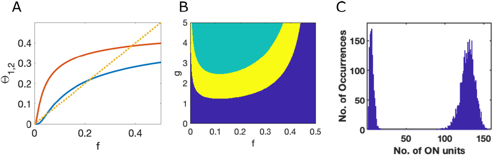
While previous work has demonstrated the existence of multistability in networks with strong self connection ( in a system with the tanh response function) in the large-N limit (Stern et al., 2014), the extent to which independent, random, zero-mean cross-connections can produce multistability in a system in which the isolated units have only a single (quiescent) stable state due to weak self-connections (blue dashed lines in Figure 1) is unknown. In order to compare how the cross-connections impact network behavior as a function of their strength, we choose parameters for each of the single-unit response functions such that the systems of isolated units () matched each other. To match prior work with we chose the threshold parameter, , such that isolated units are quiescent for and possess a bifurcation point at , above which they are bistable (Figure 1, see Appendix 2).
Figure 1. Single-unit response functions, , produce bistability at .
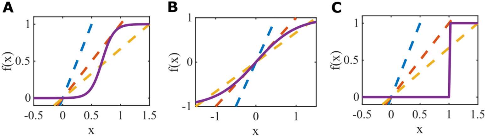
A. Logistic function with slope parameter , and threshold . B. Tanh function with slope parameter and threshold . C. Heaviside function with binary response, equivalent to the logistic function with and . Feedback curves, shown as dashed lines with blue , red , and yellow demonstrate the bifurcation from an inactive state to bistability at . Note that the bifurcation is a saddle-node in A and C but a pitch-fork in B.
2.1. Observed forms of simulated network dynamics with logistic function responses
We define the network state by its long-term activity, which can be one of four types: 1) “quiescent” meaning stable inactivity or constant low activity across all units; 2) “stable activity” meaning constant firing rates with one or more active units; 3) “limit cycle” meaning oscillating activity; and 4) “chaotic” meaning non-stationary activity, with small transient perturbations of activity reliably leading to increasing divergence of trajectories from the unperturbed one.
In many networks we find, by varying initial conditions, the existence of more than one type of state in a single network. Some networks have multiple forms of all four activity types, such as the example network in Figure 2A-D. This example network of logistic units (, , , and ) has a stable quiescent state, two stable active states, two unique stable limit cycles, and a chaotic attractor. Example trials leading to each of these distinct states in the same network are shown as a subset of units’ firing rates (Figure 2A) and in principal component space (Figure 2B). These states have similar root mean squared (RMS) firing rates, except for the quiescent state (Figure 2C). Perturbation analysis confirms the classification of each of the trials in Figure 2A-C (Figure 2D). For each trial, we simulate 100 perturbations and calculate the median RMS deviation of the perturbed simulation from the original simulation. We perform the same perturbation-based classification of activity states for 100 different random networks at the same parameter values and find that all networks show at least two forms of activity (Figure 2E).
Figure 2: All activity regimes can be observed in a single random network.
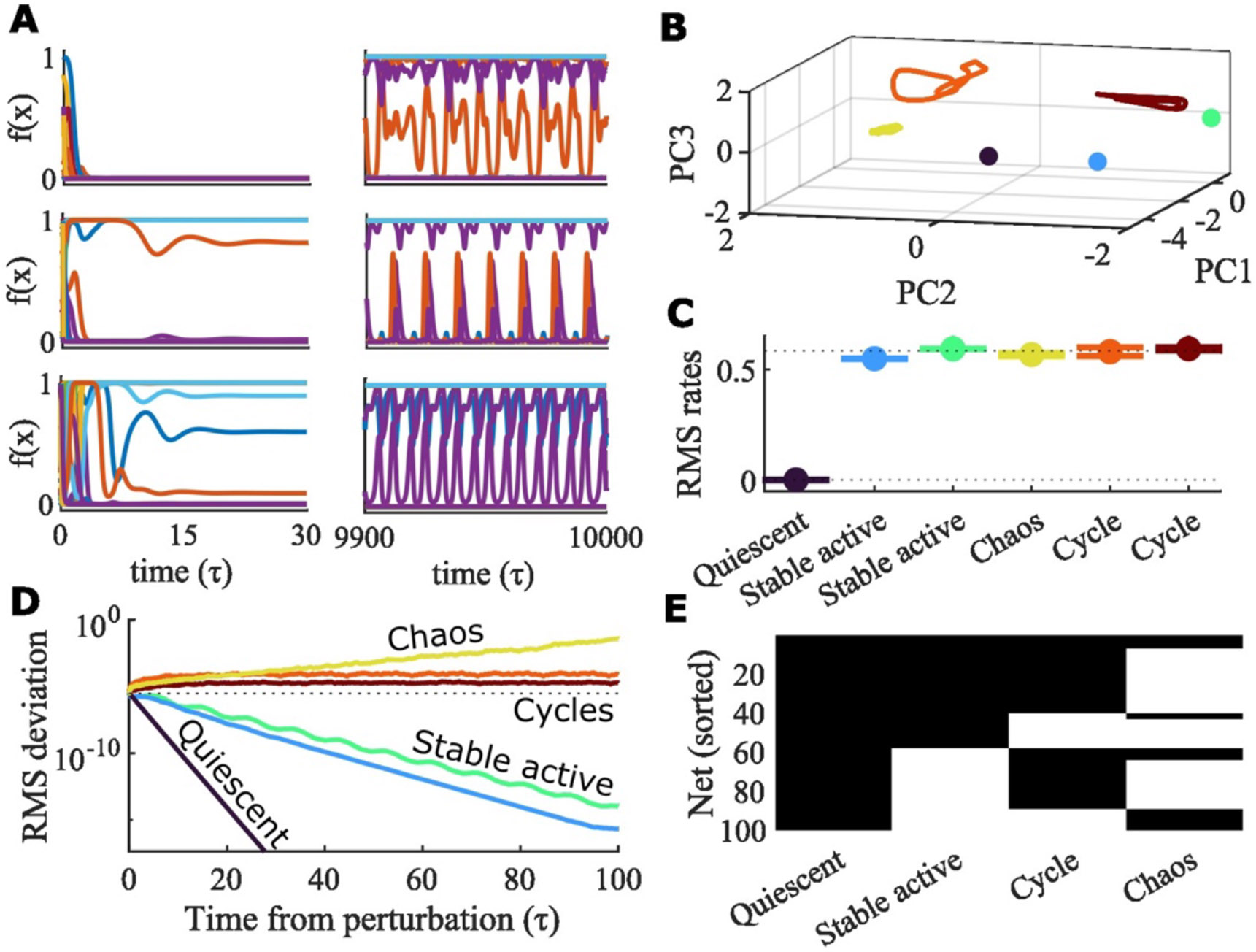
A. Different initial conditions in the same network can lead to a quiescent state, two stable active states, two stable limit cycles, and chaotic activity. For each example condition, the firing rates of a subset of units is plotted for either the beginning or end of the trial. The parameters for this network are , , , and , with a logistic response function. B. The first three principal components from PCA of the firing rates from the trials in A. Each color is a different trial. All trials converge to one of the six different activity regimes show in A. The last 100 of each trial is plotted to show the steady state activity. C. The root mean squared (RMS) firing rates of the network for each of the 6 example simulations. Colors correspond to those in B. The mean and standard deviation of the last 100 of each simulation is plotted. The dashed line represents the value predicted by analysis of the infinite- system (Section 3). D. For each trial 100 perturbations of it are simulated and the RMS deviation from the unperturbed simulation of the firing rates of all units in the network is calculated across the time from perturbation. Colors correspond to the trial colors in B and C. Dashed line indicates the initial perturbation magnitude. The median value of the 100 perturbations is plotted. E. A diverse array of mixed activity regimes is found across 100 random networks for the same parameters as the example network in A-D. Black indicates that one or more out of 100 trials produce the indicated activity type. All 100 networks have at least two types of activity. Seven out of the 100 networks have all four activity types (the top seven rows).
Of particular interest are systems without self-connections, (, such as that shown in Figure 2), because there is a well-established single transition from quiescence to chaos at , when (Sompolinsky et al., 1988). When, instead, we use the logistic response function, , which is simply a scaled and shifted transformation of the tanh function to non-negative values of firing rate, we find a richer set of states in our simulations. Perhaps surprising, circuits without self-connections can exhibit multiple stable states: sometimes having only a low activity state (a quiescent state) with a state of higher net activity (an active state) as seen for the example network in Figure 3A. Indeed, we find that for a given random instantiation of the connectivity matrix, as we scale all connections by , there is, for all 500 total networks tested in Figure 3, some range of connection strengths for which the network is multistable. Supplemental Figure 2 shows how dynamics beyond the existence of multistability changes as is scaled.
Figure 3: Smaller networks are multistable at larger g values.
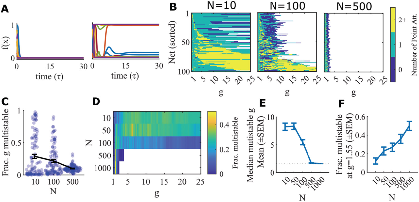
A. An example network (logistic units, , ) that has only the quiescent attractor and one active point attractor, even with no self-connections (, ). Left, a subset of units’ firing rates in a trial that converges to the quiescent attractor. Right, a trial that converges to an active point attractor. B. 100 random networks of logistic units () with no self-connections () of varying size () are simulated at each value of . The same network can gain and lose mulistability as varies. Color scale indicates number of point attractors found within 100 trials. White indicates values of that are not simulated due to computational limits, wherein each network is allotted 24 hours of cpu time. Networks tend to reach their limit at values of above a range within which the network fails to converge to a fixed point on any trial (shown in blue), indicating the likely end of the networks’ region of multistability. C. The fraction of the simulated values of at which each network in B is multistable. Bars show mean and SEM. D. Fraction of networks that are multistable across the tested values for converges with large to the narrow range expected from the infinite- limit (Section 3) around g=1.55. E. The median g value at which each network is stable. This converges to (dotted line) as network size increases. F. Fraction of networks that are multistable at increases with N.
To assess whether such states are a finite size effect, we vary the size of the network (changing ). We find that the range of over which we see such multistability at narrows with increased (Figure 3C), and converges to the same set of values centered on (Figure 3D-F). These and other results prompt us to investigate the phase space of the corresponding infinite- systems via mean field theory and stability analysis (Section 3).
2.2. Phase diagram from simulations of finite networks
To assess the likelihood of systems reaching a given type of state across phase space, we simulate 100 networks for each given set of parameters and commence simulations of each network from 200 initial conditions. Full details of simulation methods are provided in Appendix 1.
In Figure 4 we show that systems of units with the logistic response function, , can have multistability at , such that the fraction of multistable networks increases with increasing cross-coupling strength, , for large ranges of and . The switch from quiescence to multistability with increasing at low is most apparent in systems of units with binary response functions and is not so apparent for systems of units with tanh response functions. As might be expected, multistability for the logistic function with a steeper slope (, producing a maximum slope of 2.5) is more similar to that of the binary function, while multistability for the logistic function with the shallower slope (, producing a maximum slope of 1.25) is more similar to that of the tanh function (with maximum slope of 1).
Figure 4: Multistability across phase space.
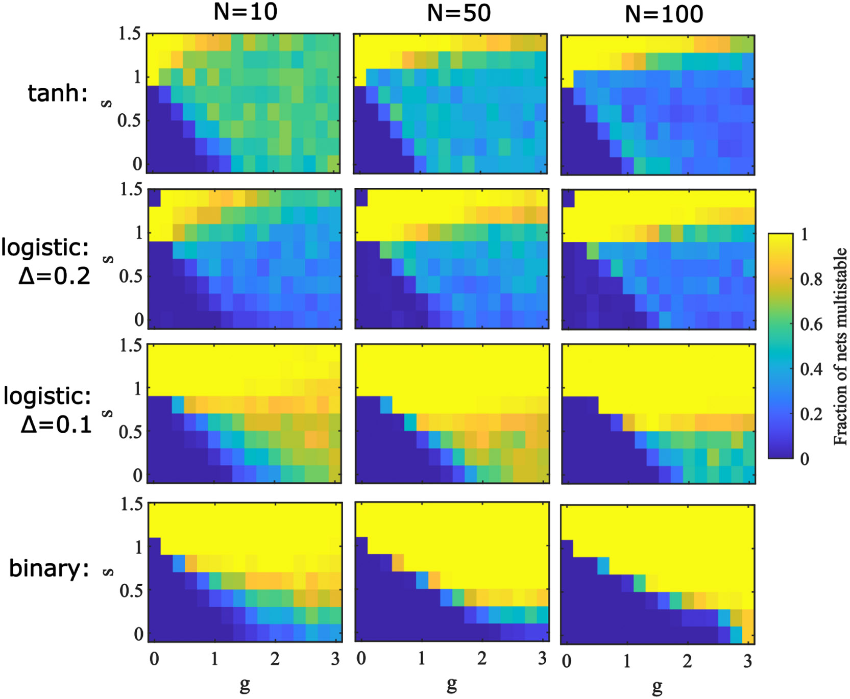
Simulation results showing the fraction of networks at different values of and with multistability. For each parameter point 100 random networks are simulated for 200 random initial conditions. Networks with 10 (left), 50, (center), and 100 (right) units are simulated with the tanh (top), logistic (middle), and binary (bottom) response functions. The large- limit of these panels is calculated in Section 3 and provided for logistic and binary response functions in Figure 6 and for the tanh response function in Figure 12.
Simulation results of Figures 3 and 4 reveal a peak as a function of network size, , in the likelihood of reaching multiple final states from a fixed (large) number of initial conditions for some parameters. However, without the exhaustive sampling of initial conditions, which becomes unfeasible at large , our lack of observation of multistability at large- in simulations is not conclusive of its absence in the model. To proceed further, we calculate results for the infinite- system in Section 3 and develop analysis of networks of units with binary response functions, which allows for finite- approximations, in Section 4.
2.3. Distribution of size of basins of attraction
The number of stable states contained in a system is a marker of its information-carrying capacity. In systems without cross-connections and strong enough self-interaction () such that each unit is independently bistable, the number of states is trivially , the maximal possible for our systems. However, without cross-connections, the ability of such circuits to process information in a history-dependent manner vanishes—how each unit responds to a stimulus is independent of the history of stimuli encoded in the activity of other units. Whereas with sufficiently strong cross-connections () even in circuits with such that individual units are not bistable, networks can be multistable (Figures 2-4) and can encode temporal properties of sequences of stimuli (Ballintyn et al., 2019; Chen & Miller, 2020; Miller, 2013). Therefore, in this subsection, we describe the results for such multistable systems with and for ease of simulations and analysis use binary units, , with .
We simulate networks from 106 distinct initial conditions sampled from the combinations of high/low activity per unit and catalogue the stable states reached in this manner. The size of the basin of attraction of a stable state is the total number of all possible initial conditions that lead to that state when single-unit activity is binary. Results for a network of 200 units are shown in Figure 5A, in which the set of stable states is ranked by the number of initial conditions resulting in that stable state. We find that some states have vastly more initial conditions reaching them compared to others, with the distribution following a power law (visible as linearity on the log-log scale of Figure 5A), known as Zipf’s Law.
Figure 5. Zipf-like behavior is observed by sampling the data, and accounted for by sampling a log-normal distribution.
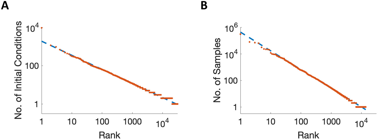
A. The number of initial conditions leading to each discovered attractor state (indicating size of basin of attraction) is recorded in an example network of size , with results ordered from the most to the least frequently visited on a log-log scale. The x-coordinate, “Rank” refers to the position of the stable state in the ordering after sorting from most frequently to least frequently visited. B. Simulations of random sampling from a log-normal distribution of sizes of attractor basins, as suggested by analysis, can account for the observed linearity on the log-log scale. Same axes as panel A.
However, it should be noted that Figure 5A is obtained by sampling only an extremely small proportion of all the possible initial conditions. The network of 200 units has potential initial states, so our simulations commencing from 106 of those initial states cover a tiny fraction of the entire state space. If the largest basin of attraction is more than 106 times bigger than many small basins, then most of the smaller basins are missed. That is, any stable state reached by < 1042 initial conditions in the network of 200 units has an attractor basin covering < 10−18 of the entire state space, so has a probability of less than one in a trillion of being found with the 106 initial conditions we used. Such considerations mean that the observed power law produced by sampling may not reflect the true distribution of sizes of basins of attraction.
While observations of power law distributions in nature are common, they often arise because a different underlying distribution, such as a log-normal distribution, is characterized across a limited range (Perline, 2005). Therefore, we analyze our system to derive a theoretical basis for the distribution of sizes of basins of attraction. Our conclusion is that the observed power-law is indeed an artefact produced by sampling a log-normal distribution of the sizes of basins of attraction with the width of the log-normal distribution being much larger than the range plotted (Perline, 2005). Our reasoning is as follows: (1) For any stable state some units (a number, ) have input in their bistable range, meaning that the unit could be stably active or stably inactive given that fixed input. If is large, the switching of such a unit does not strongly change the net input to all other units, so another stable state is reached. Such a switch to a different stable state indicates the crossing to a different basin of attraction. Across all of the distinct stable states in the network, the number of units, , with inputs in the bistable range allowing for such stable switching is distributed as a Binomial (if we ignore correlations in the identity of active units across stable states and therefore correlations across stable states in the levels of inputs received by each unit). Equivalently, the number of units, , that can be switched in any state without changing to a different basin of attraction also follows a Binomial distribution across stable states. This approaches a Normal distribution at large . (2) When a stable state has units which can independently switch activity without causing a transition to a new basin of attraction, the total number of states that can be visited while remaining in the same basin of attraction is on the order of (ignoring any mean effect of changing input to other cells produced by these individual, independent switches in activity), which is exponential in . Combining the factors (1) and (2) leads to an approximate log-normal distribution of sizes of basins of attraction.
To test if our results in Figure 5A are compatible with a log-normal distribution, we generate 107 samples from a fictitious system with 107 states whose sizes, , are distributed as , with and . Such a system is chosen to resemble the statistics, in terms of numbers of states sampled and maximum number of samples for a network of one of our random systems with .
The results of our random sampling of a fictitious log-normal system in Figure 5B, indicate that the observation of Zipf’s Law from sampling basins of attraction is, indeed, compatible with a log-normal distribution of attractor-basin sizes (see also, (Mitzenmacher, 2004; Perline, 2005)). While the two distributions are both heavy-tailed, the log-normal distribution falls to zero for very small sizes of basins of attraction, whereas the power-law distribution is maximal for the smallest basins. The intuitive reason that limited sampling of the log-normal distribution produces a power law (Figure 5B) is that many of the small basins, whose expected number of visits is less than one, either do not appear in the sampling at all (so their small numbers are not observed), or appear once or twice, in which case they add to the numbers of smallest observed basins.
In summary, the observed frequency of visits of different attractor states follows an approximate power law, but such behavior is the consequence of sub-sampling a distribution which is approximately log-normal.
3. Infinite- analysis
We follow the methods of others (Ahmadian et al., 2015; Stern et al., 2014) to develop a theory for the behavior of the network in the large- limit (). The following description of the method has a slightly different emphasis from those of others (Ahmadian et al., 2015; Sompolinsky et al., 1988; Stern et al., 2014) in part to connect to the alternative analysis that we develop in section 4 to study systems of binary units, and in part to focus analysis on the existence of multiple stable fixed points rather than the more general dynamics of the system.
In the large- limit, because each individual connection strength scales to zero, the impact of small motifs (e.g., small subsets of units with net positive interactions) and correlations in activity between units becomes negligible. Therefore, the existence and stability of any state can be assessed by assuming all units receive input sampled independently from the same distribution arising from the sum of connection strengths multiplied by the activities of units. In finite systems units with positive connections are more likely to be coactive together, rendering the simplifying assumption inaccurate. The large- limit is also then (as stated in (Stern et al., 2014)) equivalent to averaging over all realizations of the connectivity matrix, , which removes any correlation between individual units.
In the absence of any dependence on the identity of a unit, the unit label can be dropped from the formalism. The dynamical equation then describes the distribution of single-unit inputs, represented by the variable , produced by the distribution of network inputs given by a new variable, , which is summed with their self-input:
| (2) |
The distribution, , is produced by integrating the product of the distribution of responses, (which results from the distribution of total inputs, ) multiplied by the zero-mean Gaussian distribution of connection strengths (the continuous limit of the summation in Eq. 1). Given the lack of correlations between activity and connectivity in the large- limit, is produced as the limit of a sum of independent variables, each drawn from a zero-mean Gaussian distribution (albeit of different, presynaptic-rate-dependent variances), so that the distribution of is also Gaussian with:
| (3) |
and
| (4) |
where we use to represent the limit of .
Fixed points of the dynamics (Eq. 2) arise for the distribution of total inputs, , where
| (5) |
which, for a given distribution of , defines the distribution of . We define the variance of the zero-mean Gaussian distribution of as , such that
| (6) |
where must be calculated self-consistently from Eq. 4, as described in Appendix 4 (see also (Sompolinsky & Crisanti, 2018), Eqs 46-47). For the system to possess multiple attractor states, the above set of equations (2)-(6) must have multiple solutions, and those solutions must correspond to stable states. This can happen in two distinct manners:
1) Multiple solutions arise from Eq. (5) with a fixed distribution of , if the function is non-monotonic. This corresponds to individual units with fixed input from all other units being able to switch their activity. Given the response function, , has zero slope at very negative or very positive , the function has slope of +1 at these extremes and is therefore non-monotonic if for any value of the gradient of is negative, which occurs if . That is, multistability in this manner is possible if . Hence the result in (Stern et al., 2014) that if for which , multistability is only possible if . For the logistic response function, , the requirement is , which accounts for the solutions at in Figure 4.
2) It is also possible for multistability to arise due to the existence of multiple self-consistent solutions of Eq. (4) for the variance of the distribution, . Indeed, for the logistic response function, a solution with low variance corresponding to a quiescent, or low-activity state (in which activities of units are tightly clustered around ) can coexist with a solution of greater input-variance. We assess both the stability of the solution with minimal neural activity (and therefore minimal variance of ) as well as the existence of and stability of distinct solutions with higher neural activity when determining which states exist for a given set of parameters (see Appendix 4 for methods).
3.1. Phase diagram for networks with logistic single-unit response functions
In Figure 6, we show how the phase diagram depends on the slope of the logistic response function, , with the panels from A to F depicting results of increasing steepness (by lowering ). The final panel () corresponds to a binary step function and is produced by methods described in the next section. In all cases is adjusted according to Eq. A1, to ensure single-unit bistability at . As can be seen, the minimum level of allowing for multiple stable active states falls in proportion to , and in the range , the system is quiescent at , but with increasing becomes multistable. In all cases, and for all values of , the expected transition to chaos arises with large enough , though that transition is not always visible in the parameter ranges shown.
Figure 6. Multiple coexisting states in the infinite system with the logistic response function.
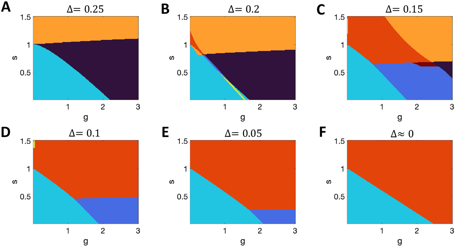
A-F. Increasing steepness of the logistic response function (corresponding to reducing ) greatly affects the phase diagram. The maximum slope of the logistic response function is . on the y-axis is the fixed self-connection strength, while on the x-axis scales the random connection strength between units. Key: black, chaos only; dark blue, quiescence + chaos; cyan, quiescence only; yellow, quiescence + single multi-unit active state; orange, multiple states all active; red, quiescence + multiple active states; crimson, chaos + multiple active states. Note that panel B describes the infinite- limit of Fig. 4 2nd row, D describes the infinite- limit of Fig. 4 3rd row, and F describes the inifinite- limit of Fig. 4 bottom row. Also, the values of at which the yellow band crosses in Panel B indicates the infinite-N limit of the simulation results in Fig. 3E-F.
In systems with (Figure 6 B-E) we find ranges of parameters for which the input distribution, , does indeed have two self-consistent solutions. Most commonly, at low , the cyan regions represent the presence of a stable quiescent state with an unstable active state, indicating the coexistence of inactivity and chaos in a given network. In a smaller range of parameters, the yellow region (Figure 6B) represents the coexistence of a stable quiescent state with a stable active state. Such multistability exists even in the absence of cross-connections () and concurs with our simulation results in Section 2.1. Indeed, the region of multistability for a network with spans the value of , at which multistability is observed at larger- in simulations (compare Fig. 3E-F with Fig. 6B). Therefore, even without the self-excitation needed for individual units to be bistable with sufficient input, the network can possess multiple stable states, with the two distinct states resulting from and causing two distinct population-mean (and mean-square) firing rates (Fig. 2C) and two distinct population input distributions.
3.1.1. Accounting for extreme tails of a Gaussian in the Infinite System
We define a stable state as quiescent if all units have activity of less than half of their maximum (as units have non-zero activity with zero input some low level of activity is always present). In systems where bistability is possible () all units must receive input corresponding to the lower branch of the bifurcation curve for a stable quiescent state to exist. In the infinite system, any requirement of all units raises a subtle issue that we address in this subsection (and in Appendix 4 and Figures 13-14).
, the probability of any unit receiving a given network input, follows a Gaussian distribution. When all firing rates are very low, the variance, , of the Gaussian distribution for is very low but is non-zero. The probability of a unit receiving input with a magnitude , that is many () times greater than the standard deviation, , is vanishingly small (e. g. if the probability is less than 10−9 and if the probability is less than 10−18). However, for any finite the probability is strictly non-zero for a cell to have input greater than any finite value, so an infinite system will always have units whose inputs exceed the specified value of . Therefore, in a system in which , the quiescent state is unstable for an infinite system, unless precisely. Yet, for any circuit of a biologically feasible size, we can define a and require the values of input at the bifurcation points, , to be within the range , in order for the quiescent state to be defined as unstable. In this manner, we can study a system in which we ignore correlations (an approach strictly only correct in the infinite- limit) but at the same time define states that would be present in a large finite system with results accurate (for 99.9% of networks) for network sizes up to (with ) or even (with ).
A similar issue arises when we consider whether a system has multiple stable active states. The number of such states depends (exponentially) on the number of units receiving input in the bistable range (between the two bifurcation points of such that the unit could be either active or inactive for that level of input). Whenever there is a pair of bifurcation points (), the argument from the previous paragraph again indicates that in an infinite system there is always a unit with input in that range. However, while in the infinite system the network is multistable, for any realistic system—even a large one, of the sizes discussed in the previous paragraph—it may be very unlikely that any unit receives sufficiently extreme input, so we use the same value of to indicate multistability as we do for stability of the quiescent state.
Given the results depend on choice of , in Appendix 4, Figure 13 we replot the phase diagrams of Figure 6B and 6D for distinct levels of , while using a standard of for most phase diagrams. For example, with , a large network of 106 units has a probability of only 0.001 of behaving differently from that indicated in the phase diagram (and a network of 103 units has a 1 in a million chance of behaving differently—the fewer the units in a network, the less likely that at least one of those units receives excessively high input). In the limit of , the system has a discontinuity moving away from on the y-axis, as while the region of multistability approaches (for ) throughout this paper we have set the threshold, , such that disconnected units () are only bistable if .
By contrast, for the network of units with tanh response functions of maximum gradient greater than 1 (i.e., with low and higher to maintain the single-unit bifurcation maintained at ) the output of units with zero input is close to −1 (rather than close to 0 as it is for units with the logistic response function). Such maximally negative output produces a larger variance of inputs across units, such that multistability is more common at very low cross-connection strength (see Appendix 4, Figure 12E-F). Therefore, while the choice of still impacts the phase diagram for those reasons discussed above, it does so to a much smaller extent in networks of units with tanh response functions (see Appendix 4, Figure 14).
3.2. Multistability without self-connections
Multistability without self-connections (i.e., with ) is possible in all networks with logistic response functions if we allow to vary (or equivalently apply uniform input, varying in Eq.1). To demonstrate this, in Figure 7A we show the phase diagram as a function of and for a system with logistic response functions with parameters and . Note that for the logistic response function is equal to . Systems with different produce identical figures if the two axes are scaled by the same factor as (data not shown). As can be seen, the region of coexistence of quiescence with chaos is contiguous with a region of coexistence of quiescence with an active state in which any fixed point is stable. These two regions, which represent networks with multiple stable solutions for the self-consistency of the distribution, , and hence multiple stable solutions of population-averaged activity, are not present if the response function is (Figure 7B).
Figure 7. Phase diagram without self-connections.
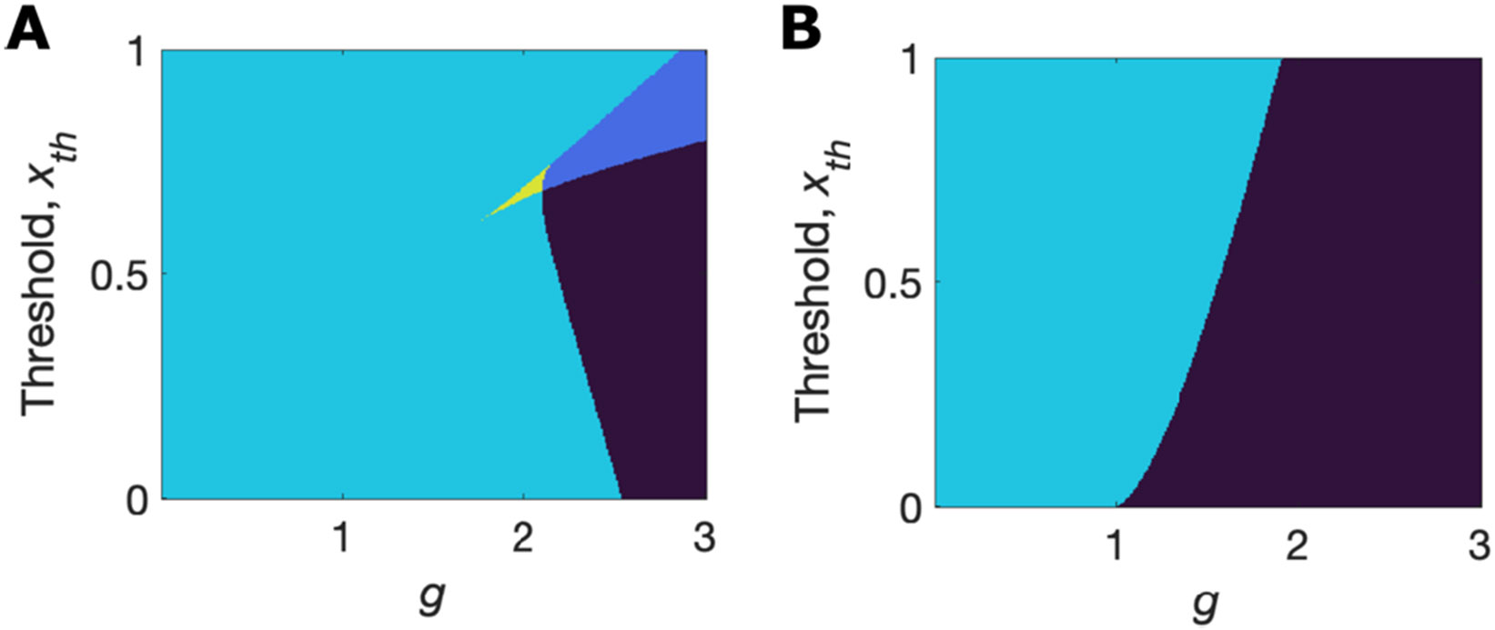
A. Networks of units with logistic response functions do not require self-connections to be multistable. B. Networks of units with tanh response functions are only monostable or chaotic when they lack self-connections. (Black = chaotic; dark blue = chaotic + stable quiescence; cyan = stable quiescence only; yellow = stable quiescence + active state in which any fixed point is stable.)
The two response functions, and , have a key difference that leads to them producing qualitatively different behavior. For the logistic response function, the minimal absolute value of coincides with the minimal gradient of the function: if is low then is low. At low firing rates, increases with increasing as the function is supralinear. Hence for a network of units with logistic response functions, it is possible for a narrow range of inputs to produce a stable narrow range of low activity (maintaining low inputs) while in the same system a larger range of inputs can lead to an instability with increasing activity. With even higher activity a stable solution is reached at which a significant fraction of units responds stably with much larger activity (maintaining high network input) where is low again. However, for the tanh function, the gradient of the response function decreases monotonically with a change in activity from zero, so solutions with high mean activity can only be stable if the solution with zero activity becomes unstable. Graphically, the reason for this difference in network behavior is the same as that depicting different single-unit behavior in Figures 1A and 1B: Single units with a logistic response function have both stable high activity and stable low activity following a saddle-node bifurcation with increasing feedback (Figure 1A) whereas single units with a tanh response function only have high stable activity once the zero-activity state becomes unstable through a pitchfork bifurcation (Figure 1B).
4. Analysis of networks of units with binary response functions
For a system with the binary response function for units, , the analysis simplifies, because a state is stable if all active units have input from other active units exceeding by a small amount, , and if all inactive units have summed input from the active units less than by a small amount, . That is, if inputs to units are perturbed by a small amount up to , the system returns to its prior state, so the value of determines the smallest distance of a stable fixed point from its separatrix to a new basin of attraction. Such stability arises because for all but an infinitesimal part of the domain of the Heaviside function (see Eqs A4-5, Appendix 4). For this section we take to be an infinitesimal positive quantity.
We define as the number of active units, each with an activity of 1, so the above requirements on network inputs correspond respectively to conditions on the sum of of the connection strengths to each of active units and on the sum of connection strengths to each of the inactive units. By taking the large- approximation these sums of and connections strengths can be treated as independent draws from a Gaussian distribution with mean of zero and whose variance is and respectively. A solution with active units can then be assumed to exist if, given independent draws from a Gaussian of unit variance, the top draws, when multiplied by are greater than (high input to active units) while the remaining draws, when multiplied by are less than . This is equivalent to the requirement that the greatest sample out of samples, , from a unit-variance, zero-mean Gaussian distribution lies in the range:
| (7) |
where we assume and (which holds in our standard system with so long as , so the results of Section 4 are restricted to this parameter region in which independent units are not bistable).
The requirement of Eq. 7 can be calculated using the methods of order statistics (David & Nagaraja, 2003), which we follow for the Gaussian distribution, defining
such that
| (8) |
Combining Eq. 7 with Eq. 8, we have a stable state with of units active with a probability given by:
| (9) |
We then calculate the probability a system has at least one stable state with multiple active units, and so is multistable (as the quiescent state is always stable for ) for a given system size, , via:
| (10) |
(there is only an absence of multistability if it is absent for all possible numbers of active units, ). While Eq. 10 is an approximation as it assumes is independent for different values of , we show in section 4.2 that in the large- limit the approximation becomes exact, as becomes either 0 or 1, so that is also either 0 or 1, and we have multistability with probability 1 if and only if it arises with probability 1 for some value of : that is .
4.1. Finite- results of analysis with binary units
The simulation results presented in Section 2 (Figure 4) suggest that, for some values of the parameters and , networks of intermediate size have the greatest probability of multistability. Given the increasing likelihood of missing stable states as increases using simulation methods, such a simulation result may be incorrect due to undersampling at large . Therefore, we use our approximate analytical methods for networks with binary units to address the -dependence of the probability of multistability, by solving Equations (8)-(10) above, and setting .
In Figure 8A-C, we show that for small networks of (green curve), (yellow curve), and (blue curve), for which we can exhaustively test all initial conditions and therefore find all stable states in simulations, the approximate analytical method (solid line, which plots Eq. 9) matches the simulated data (crosses). Moreover, in Figure 8D-F, when we use Eq. 10 (red lines) to estimate the probability the network is multistable, the simulated results (crosses) are remarkably close to the analytic approximation. Such a result is surprising, as one would expect a positive correlation across networks and the numbers of stable states, rendering the approximations used in the analysis inaccurate. The blue lines in Figure 8D-F are the results for a correlation of +1, in which the network’s probability of multistability is simply the maximum across possible states and is much farther from the data than the analysis assuming zero correlation (the red line). Nevertheless, across all methods, in Figure 8D-E, we do indeed find that the probability of multistability peaks at intermediate network size, remarkably reaching values of approximately 1 for , , before falling to zero at large network size ().
Figure 8. Numbers of stable states in finite binary networks.
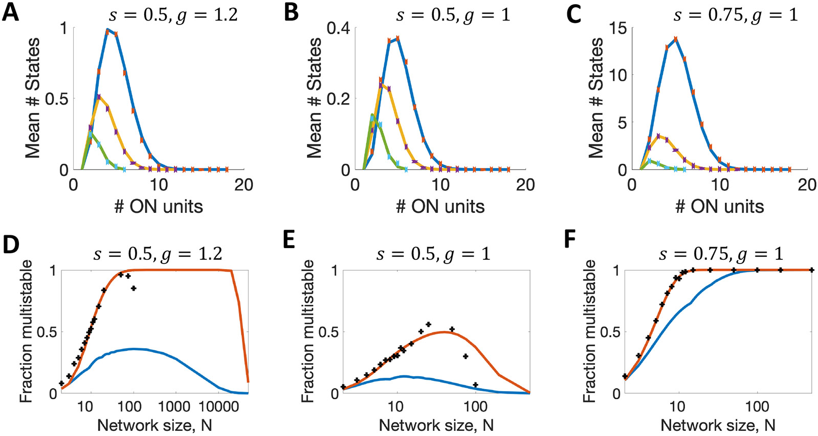
A-C. Expected number of stable states with active units when (green), (yellow), , blue. Continuous lines are from analysis (Eq. 9), and points are from simulations. D-F. Probability a network is multistable as a function of network size, . Top curve uses Eq. 10, lower curve uses . Crosses are simulated data points in all panels, and are an undercount at large .
4.2. Large- limit of the system with binary units
In the large- limit, equations (8)-(9) can be simplified. First, we note that
| (11) |
is the Binomial probability for achieving outcomes from independent selections, with individual probability of outcome, . In general, the probability has a peak at the integer value of closest to , with a standard deviation of .
If we define with as well as , then the integration limits for in Eq. 9 become and . Also, for large , the Binomial probability term approaches a Dirac delta-function at the value of , as it’s standard deviation in scales as . Therefore, in the large- limit, if the integration range over contains the value where and otherwise. Algebraically this becomes a requirement for a stable state that lies between two thresholds, and , which each depend on :
| (12) |
Figure 9A shows that there are two ranges of satisfying the above two inequalities (where the yellow dotted line denoting is above the blue curve denoting and below the red curve denoting ) for the specific values of , , and , while setting . Figure 9B shows that for a wide range of the possible numbers of active units in a stable state is split into two distinct ranges. Simulation results in Figure 9C demonstrate such bimodality in numbers of active units for a similar network ( and ) with .
Figure 9. Number of active units in stable states is bimodal.
A. The two complementary error functions producing the bounds on fraction of active units, , from Eq. (12) (infinite system with , , , and ). Dotted yellow line shows the value of . Where the red curve is above the dotted yellow line active units are stably active, but otherwise not. Where the blue curve is below the dotted yellow line, inactive units are stably inactive, but otherwise not. Note the two distinct ranges of in which the dotted yellow line is above the blue line and below the red line. B. Across a range of for the same system as A, the allowed range of for which stable solutions are possible, as indicated in yellow, splits in two. In the blue region the active units are unstable, while in the green region the inactive units are unstable. C. Simulations of a network (, , , and ) of size from initial conditions of varying numbers of active units lead to final stable states with a bimodal distribution in the number of active units.
Given that at it is always true that (because of the limited range of the complementary error function) the criterion for Eq. 12 to have a solution for some value of is the requirement for some , which leads to a minimum value of at which the lines and meet at a tangent. The critical value occurs where such that, as a function of and with , multistability arises in this system if (which matches the boundary shown in Section 3, Figure 6F).
As approaches zero, the range of with allowed solutions shrinks toward the line where . For , there are two such solutions, which are distinct crossings of the line (see Figure 9A). The distinct solutions indicate two separate ranges for the possible number of active units in stable attractors. In the example shown in Figures 9A and 9B, solutions are possible in two ranges, either with a very low fraction (<5%) of units active or with a fraction in the range of 30%-40% of units active. The two distinct ranges are also visible from simulations as a bimodal distribution in the numbers of active units in stable states following random initial conditions (Figure 9C).
A lower bound on the fraction of active units arises, because with few active units there is too little network input to activate those units. The upper bound arises because half of the units receive net negative input, so cannot be stably active if , and only a subset of those units receiving net positive input receive an amount greater than , as needed to be stably active. The bounded region in which active units have sufficient input to remain stably active can contain within it a separate bounded region of instability (Figure 9) because the random network input can be sufficiently strong that some of the inactive units (of which there are more than there are active units) receive too much input to remain inactive.
5. Discussion
Firing rate models of neurons are valuable because they can reveal the likely states of a neural circuit in a relatively simple manner and can be solved rapidly. The foundation of a firing rate model is the input-output function (the response function) of a unit (representing many neurons), which is typically designed to have bounded outputs over the domain of inputs. For its ease of mathematical manipulation, the hyperbolic tangent function, , has been used with great success, most notably for first demonstrating the transition from quiescence to chaos as the strength of random cross-connections increases (Sompolinsky et al., 1988; Stern et al., 2014). The negative portion of , while it cannot correspond to negative firing rates, could be considered representative of a group of mixed excitatory-inhibitory neurons in which the mean activity of inhibitory neurons exceeds that of excitatory neurons. Equivalently, the response function can represent the saturating output current of a unit with linear activity, , in which negative and negative also represent a dominance of inhibitory neurons within the unit.
Given the function is simply a translated version of the function , one might expect that analysis of a system with units responding via the one function would provide all the qualitive insight necessary to understand the behavior of a system with units responding via the other function. However, this is not the case. A qualitative disconnect between the behavior of a system of neurons with and that of a system with has been shown by others (Figure 4b of (Touboul & Ermentrout, 2011)) whereby a Hopf bifurcation disappears as the response function of units is parametrically shifted up toward non-negative values. In our analyses, we find two qualitative changes. The first is a shift in phase boundaries leading to the result that random cross-connections, whose mean value is zero, can produce multistability in a system in which single units are not in of themselves bistable.
Second, we find the possibility of bistability via distinct stable solutions for the self-consistency of the variance of the input distribution in the infinite system, corresponding to differences between solutions in the population-averaged firing rates. Such alternative self-consistent solutions can lead to multistability arising from random, zero-mean, cross-connections even in systems without self-connections (Figure 3 and Figure 6B). The distinct self-consistent solutions, with different variances in the input currents, correspond to states with distinctly different numbers of active units. Figure 9 indicates a similar bimodality in the numbers of active units in simulated binary-unit systems and is coupled with an analysis of how such bimodality arises in the system.
We find a subtlety when taking the infinite limit of our system using the logistic response function, in that there is a strict discontinuity between results with and those with (where scales the strength of cross-connections and is an infinitesimal positive quantity). The reason being that for non-zero , there is a non-zero (even if miniscule) probability that the within-circuit input to a unit, which is drawn from a Gaussian with width proportional to , is sufficiently strong to render that unit bistable. However, when the bifurcation point is many tens of standard deviations above the zero mean of the Gaussian distribution, the probability becomes infinitesimal and is irrelevant in any real or simulated system, even with billions of units. For similar reasons, the strict mathematical limit has a discontinuity when altering the width of the logistic function from to . If, instead of producing a phase diagram, with a sharp boundary for multistability, we focused on the entropy of the system (the log of the number of stable states) scaled by system size, , such discontinuities would disappear as the entropy would reduce continuously and smoothly (and rapidly) from the boundaries of multistability shown in Figure 6, to a tiny value before becoming strictly zero at or .
Multistability, when exhibited in a model as a set of discrete stable fixed points, may seem unlikely in any cortical circuit given that activity is never static in vivo. However, a network based on multiple fixed points, but with randomly timed transitions between them, can match the observed data in a number of systems (Ballintyn et al., 2019; Ksander et al., 2021; La Camera et al., 2019; Mazzucato et al., 2019; Miller, 2016; Miller & Katz, 2010; Moreno-Bote et al., 2007; Recanatesis et al., 2022). Moreover, analyses of patterns of neural spiking in vivo have, in many cases, shown that a discrete state-based formalism better matches the data than a formalism assuming continuously changing, graded activity (Abeles et al., 1995; Miller & Katz, 2010, 2011; Ponce-Alvarez et al., 2012; Sadacca et al., 2016; Seidemann et al., 1996).
While the strengths of connections between units are treated as independent random variables for ease of analysis in this paper, in practice there is internal structure in the connectivity among neurons, even between excitatory pyramidal cells (Song et al., 2005; Stepanyants & Chklovskii, 2005). Moreover, connections from cortical neurons typically have fixed sign (all excitatory or all inhibitory) according to neuron class, a feature that can change the behavior of random networks (Rajan & Abbott, 2006). In our work, we consider a firing rate model unit as representing the mean rate of a cluster of many neurons (as is necessary to omit the pulsatile spike interaction from simulations) so the net interaction between units can be of either sign according to whether the dominant connections are excitatory-to-excitatory, or excitatory-to-inhibitory, etc. Moreover, much of the nonrandom cortical structure can be accounted for by considering the intra-cluster connectivity to be distinct from the inter-cluster connectivity (Bourjaily & Miller, 2011) as we do here.
Our main conclusion is that multistability can be produced via random, zero-mean cross-connections in neural circuits without the exceptionally strong self-connections needed to produce bistability in a single cluster of neurons (a unit in a firing-rate model) so long as the neurons without input have a low firing rate and if rate increases supralinearly with low input.
Acknowledgments
The authors are grateful to NIH-NINDS for support of this work via R01 NS104818 and to the Swartz Foundation for a fellowship to SQ. We acknowledge computational support from the Brandeis HPCC which is partially supported by the NSF through DMR-MRSEC 2011846 and OAC-1920147. SM is grateful to Merav Stern for helpful conversations in the early stages of this work.
Statements and Declarations.
The work was supported by a grant from the National Institutes of Health, R01 NS104818, by the Swartz Foundation, and by the Neuroscience Graduate Program of Brandeis University. We acknowledge computational support from the Brandeis HPCC which is partially supported by the NSF through DMR-MRSEC 2011846 and OAC-1920147.
Appendix 1: Monte Carlo simulation method
Our standard procedure is to simulate 100 different realizations of the connectivity matrix to produce 100 random networks for a given parameter combination. For each connectivity matrix, we then complete sets of multiple trials, each trial with a distinct initial condition (100 trials for perturbation analysis in Figure 2 and for scaling in Figure 3; 200 trials for parameter grids in Figure 4; and 106 or 105 trials respectively for the networks with binary units in Figures 8 and 9) . For the small () networks with binary units in Figure 8 all combinations of initial conditions are used with each unit at an initial rate of its minimum or maximum.
The continuous models are simulated using MATLAB’s ode45 function. Each trial is simulated until either a maximum simulation time is reached (5,000 for Figure 3 and 10,000 for Figure 4), or until a stopping condition is reached in the case that the maximum at a give timestep is less than . If this stopping condition is reached, then the activity is considered to have reached a stable state because the network possesses a point attractor at that set of firing rates. Logistic units are classified as active if their firing rate exceeds 0.5. Tanh units are considered active if the absolute value of their rate exceeds 0.001. For the continuous models, typically the first trial is initialized with inputs near zero, to test if the quiescent state is stable. For all subsequent trials, the initial rates of the units are set to a uniform random distribution over 0 to 1 and transformed by a logistic function with and .
For the perturbation analysis, each trial of each network is simulated for a duration of 21,000 . Then, at each of 100 linearly spaced time points between 20,000 and 20,800 10% of the units’ firing rates are randomly perturbed upwards or downwards by 10−5 and the simulation is then continued from each such perturbed state for 200 . The root mean squared (RMS) deviation of the perturbed simulation from the original simulation quantifies the extent to which the perturbation causes a divergence in activity. The median RMS deviation over the 100 perturbations is then used to classify each trial as a point attractor, a limit cycle, or chaotic. The median RMS deviation exponentially decays for point attractors, exponentially increases for chaos, and increases but reaches a plateau at a low level for limit cycles. Classification thresholds are determined by the square of the correlation (R2) of a linear fit to the exponential RMS deviation and the magnitude of the RMS deviation averaged between 190 to 200 post-perturbation. Trials with final RMS deviations below half the magnitude of the initial perturbation and with no units having a change in their firing rate exceeding 10−4 in the last 10 of the unperturbed simulation are classified as point attractors. To classify trials as chaotic vs limit cycles, a classification boundary is determined as a function of each trials’ linear fit R2 and final RMS deviation. Trials above the line are classified as chaotic. This boundary allows the separation between these two dynamics because it accounts for both chaotic trials that very quickly converge to a large RMS deviation (large RMS deviation and low R2) and chaotic trials that have a slower exponential increase in their RMS deviation (lower RMS deviation at 190 to 200 but high R2). Final activity states of the unperturbed simulations are used to confirm these classifications.
Appendix 2: Choice of single-unit input threshold
For comparison across systems with distinct single-unit response functions, , we adjust the offset, , such that a single unit becomes bistable with self-connection strength of , in all cases.
For the logistic response function, such a requirement means that a saddle-node bifurcation occurs at , with unstable and stable fixed points colliding at given by such that and such that . Combining these equations and using the result for the logistic function that leads to the requirement:
| (A1) |
For the binary response function, , we have , which can be seen from equation (A1) in the limit .
For the hyperbolic tangent response function, , a similar derivation leads to
| (A2) |
which yields if , matching the simplest response function, , and as with the binary response function, if .
Appendix 3: Networks with multiple states and no self-connections
Here we verify that the majority of simulated networks up to a size of show multiple point attractors, while the range of in which such multistability exists converges with increasing to the narrow range found in our infinite-N analysis ().
Figure 10: The dynamic regimes of individual networks changes as g is scaled.
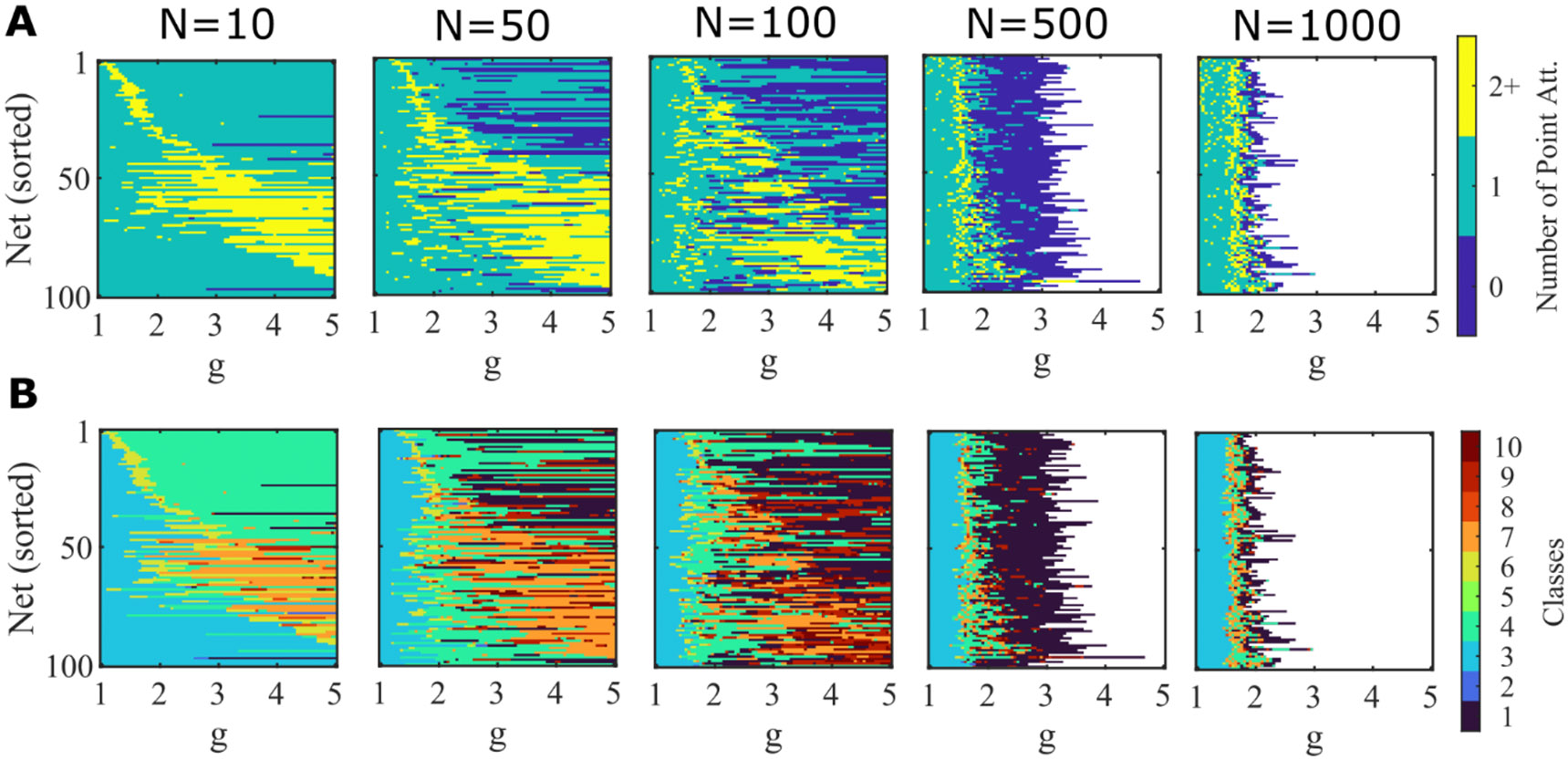
A. Similar to Figure 3B, but for networks simulated over a smaller range of g. 100 random networks of logistic units () with no self-connections () of varying size (N=10, 50, 100, 500, 1000) are simulated at each value of g. The same network can gain and lose mulistability as g varies. Color scale indicates number of point attractors found within 100 trials. White indicates values of g that are not simulated due to computational limits. B. The same simulations as in A, but where color now indicates the classification of the set of activity observed across the 100 simulated trials. 1, no trials converge; 2, stable quiescence + some trials fail to converge; 3, only stable quiescence; 4, only a single stable active state; 5, some trials don’t converge + stable quiescence + at least one stable active state; 6, stable quiescence + a single stable active state; 7, multiple stable active states + no stable quiescence; 8, multiple stable active states + stable quiescence; 9, some trials fail to converge + a single stable active states; 10, some trials don’t converge + multistable.
Appendix 4: General mean-field methods
Self-consistency of solutions
The self-consistent solution of Eqs 2-6 is straight forward when is a monotonic function such that there is a one-to-one mapping from to following Eq. 5. The variance, , of the Gaussian distribution of , is the only parameter to be calculated, so the iteration is one-dimensional and in our experience always converges using the MATLAB solver “fzero”. The procedure is, given an initial value of , which defines (from Eq. 6) we numerically integrate over . At each value of we calculate by numerically inverting (from Eq. 5), and hence calculate and . Multiplication of by combined with the numerical integration leads to (where we indicate its dependence on because depends on ). For a self-consistent solution (Eq. 4), so we require the solver to find the zero-crossing of when calculated in this manner. We use standard numerical integration grids of 5x10⁴ points and test integration grids that are 10-fold finer for select parameters to ensure the results are numerically accurate. Since multiple solutions for are possible, we systematically vary initial conditions and the bounds of to find zero crossings, to ensure we reach all solutions. We only ever find one solution or three solutions. With three solutions we only count the lowest and highest values of as the intermediate value corresponds to an unstable solution of Eq. 2.
In situations where is non-monotonic, across a range of values of the solution is not single-valued. In this case, an additional parameter is the point of the range of at which we switch from one branch of to another when calculating . We test for solutions with different switching points in order to assess whether any solution is stable, as described in the later subsection, Multiple Solutions. In such non-monotonic situations we use finer integration grids of 5x10⁵ points because of the sensitivity of near turning points of the curve. We also test integration grids that are 10-fold finer for select parameters to ensure the results are numerically accurate. (See https://github.com/primon23/Multistability-Paper/ for full code).
Stability of solutions
To test whether a distribution of the interacting variables, , produces a stable fixed point, it is necessary to obtain information about the eigenvalues of the Jacobian matrix of the dynamical equations expanded linearly about the fixed point (Strogatz, 2015). If all such eigenvalues have a negative real part then the fixed point is stable. Linearization around a fixed point, , yields
| (A3) |
where is a diagonal matrix with elements equal to the corresponding derivatives of the response function, , and is the unit variance, zero mean, Gaussian connectivity matrix.
We follow the methods of others (Ahmadian et al., 2015; Stern et al., 2014) who showed that eigenvalues of such a system are found at the complex values, , where
with
In the large- limit the sum within the Trace becomes an integral over the distribution of , to yield the criterion (Ahmadian et al., 2015; Stern et al., 2014):
| (A4) |
As noted by (Stern et al., 2014), for the system to be stable it is necessary that Equation A4 is not satisfied for any with , which allows us to assess the case where and note that any non-zero contribution to increases the absolute value of the denominator in Eq. A4, so if there are no eigenvalues with there cannot be any on the imaginary axis. Therefore, in general we require, for there to be no eigenvalues with positive real part, that
| (A5) |
where we have substituted for and . We have also assumed that the function in the denominator, , is positive, as any negative portion of the function means there is a divergent positive contribution to the integral for some with .
Verification of analytic methods
While we follow exactly the methods of others (Stern et al., 2014) in the infinite- analysis, the validity of ignoring the index of units in a mean-field manner has not been established rigorously for static solutions of the dynamical system. In this subsection we justify our method.
First we explain why, for a specific set of firing rates, each unit experiences network input that corresponds to a random sample, from a Gaussian distribution of zero mean and variance equal to : Each input from one presynaptic unit to one postsynaptic unit is a random sample (independent of that of other units given that connections are independent) from a Gaussian of zero mean, and the sum of such Gaussian samples (to provide the total input) is equal to a Gaussian sample from a distribution with zero mean and variance equal to the sum of variances of individual samples. Since self-connections are treated differently, total input to each unit is sampled from a slightly different distribution of connections, so for small- the variance of the Gaussian distribution used in sampling is slightly different for each unit. However, the impact of one input is negligible in the large- limit.
If one input distribution satisfies the self-consistency requirements of Eqs. 2-6 and is stable, then the population activity is stable in the statistical sense (as an ensemble of rates), but that does not mean that each unit has a stable fixed firing rate. While the methods of Ahmadian et al. (Ahmadian et al., 2015) described in the preceding subsection, allow us to determine whether a fixed point of the dynamical system is stable, we must still establish the existence of such a fixed point. We use the rest of this subsection to justify our claim of multiple stable fixed points, first in the case that the rates of individual units are single-valued in their network input ( is monotonic in ), and to show that multiple stable fixed points are possible if the circuit has two stable distributions of .
Figure 11. Simulation results for networks with increasing converge to the infinite- analytic results.
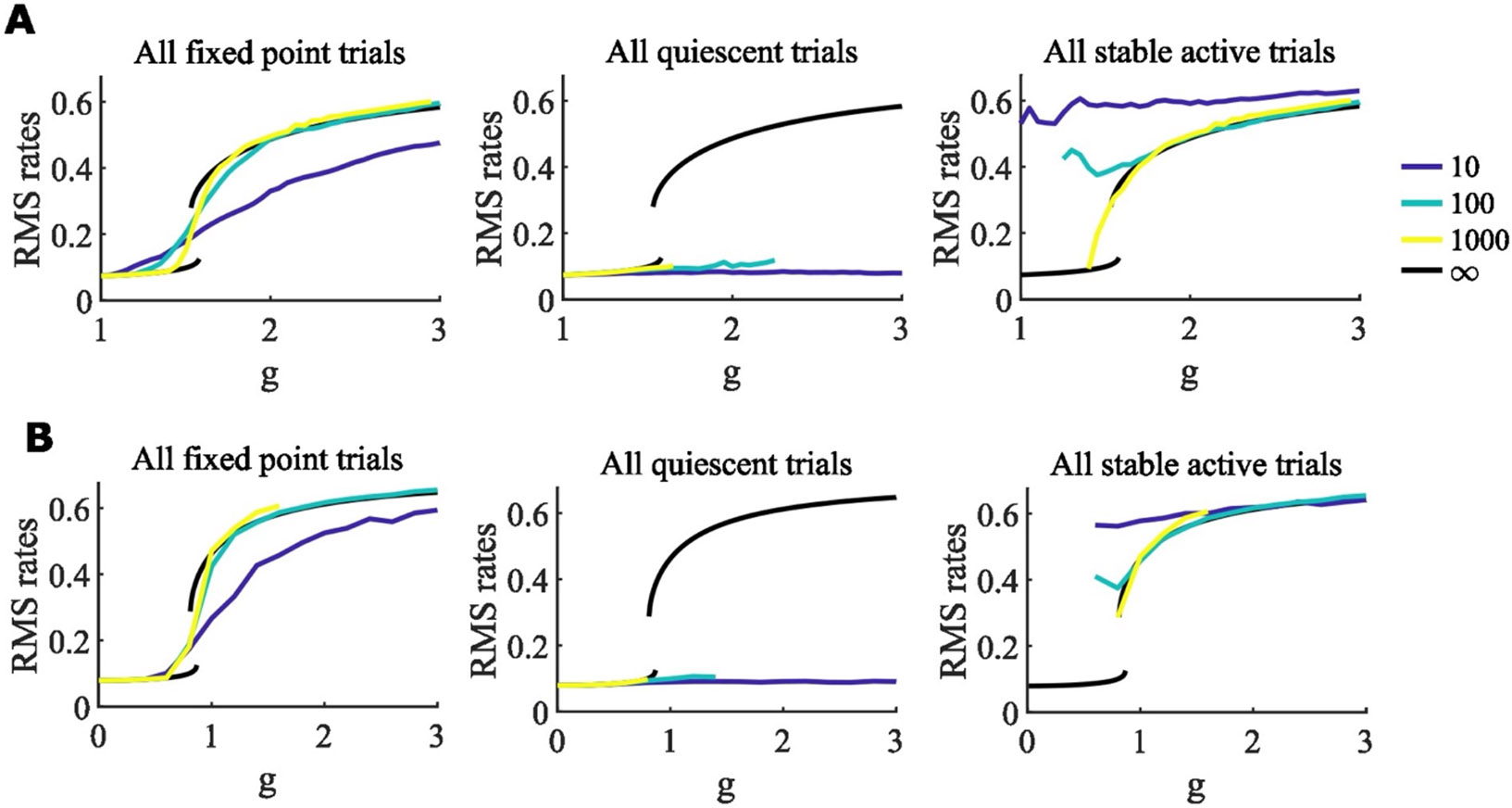
A-B. Data for all simulations reaching fixed points from 25 simulations of 100 networks are averaged in the first column and separated out into states in which all units have low rate (quiescent, middle column) or one or more units are active (right column). Network-size of simulations is indicated by the color of the curve, with the root-mean-square of firing rates, , taken across units in each network. These curves are compared with calculated for the infinite- network (black curves). Units have logistic response functions with A. , , and B. , .
In Figure 11, we show that the self-consistent solutions for the root-mean-squared firing rates, and hence the variance of the zero-mean input distribution, of stable fixed points in simulated networks approaches that of the infinite- calculations as increases (see also (Cabana & Touboul, 2018), e.g. Theorem 5, for justification).
As increases, the phase diagrams in Figure 4 indicating multiple stable fixed points approach the corresponding infinite-N limits in Figures 6 and 12.
As increases, the range of at which we find multistability without self-connections (Figure 3) in simulations matches the range found using the infinite- methods (Figure 6B, x-axis).
As a heuristic argument, for a given stable distribution of inputs, there are combinations for ordering the units by firing rate. For the system to have a stable fixed point one of those combinations must provide inputs that are ordered in the same manner. The probability of any individual order matching the required order is . Therefore, for large- this leads to a probability of of there being one or more stable fixed points, with the number of fixed points following a Poisson distribution of mean 1. Indeed in Fig. 2E, the number of networks with at least one stable active attractor state is not significantly different from the expected number from this argument (58 out of 100 from simulations versus 63 out of 100 expected, but note that the sampling in simulations can be an undercount). Moreover, if we count the number of distinct stable active attractor states in each network, we find the numbers 42, 40, 13, 4, 1 for 0, 1, 2, 3, or 4 states respectively, a result which is not significantly different from a Poisson distribution with mean of 1(, Kolmorogov-Smirnov test).
In cases where the firing rates are always single-valued in the external inputs ( for networks of logistic units) the stable solutions may not be fixed points, as discussed in item 4). However, for parameters whereby a finite fraction, , of units have two possible stable firing rates given their external inputs, even allowing for correlations, there become an infinite number () of extra state combinations that can produce the desired ordering of inputs, suggesting the probability of multistability is on the order of , which approaches 1 with increasing and .
When we use these methods to analyze networks in which units have the response function , our results exactly match those of prior work, including the well-established transition to chaos at if (Figure 12A).
Figure 12. Phase diagram for networks with tanh units.
A. Results with replicate those of (Stern et al., 2014). B-F. Region of multistability increases to lower while remaining only for on the y-axis. (Black = chaos; cyan = quiescent only; orange = multiple active stable states.)
Multiple Solutions for
can have more than one value based on the solutions for some values of . This requires that is a non-monotonic function, which occurs if max (to produce a region of negative slope in the function ). The need for a region of negative slope arises because in all cases considered here at large positive or negative values of , and has a slope of +1. In cases of multiple solutions for care must be taken in the choice of , as while stability is enhanced by choosing the solution with the lower value of , such a choice can lead to the lower value of for some response functions (but not if ) which can lead to the self-consistent solution for the distribution of to become too narrow to support multistability, as discussed below.
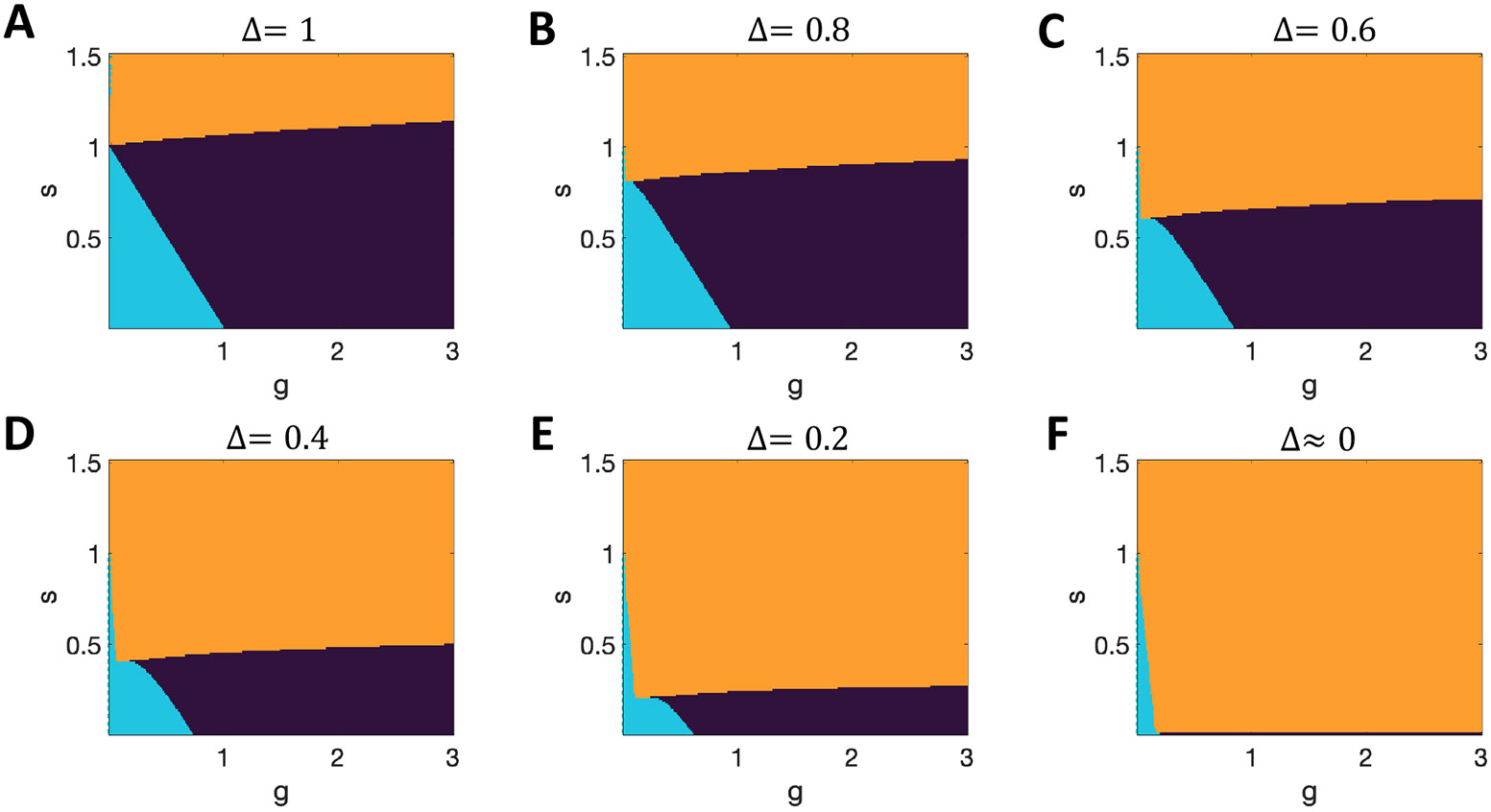
Figure 13. Impact of the criterion for multistability in networks with logistic units.
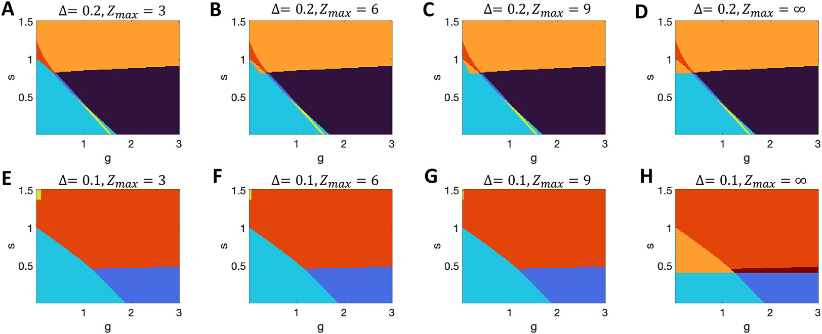
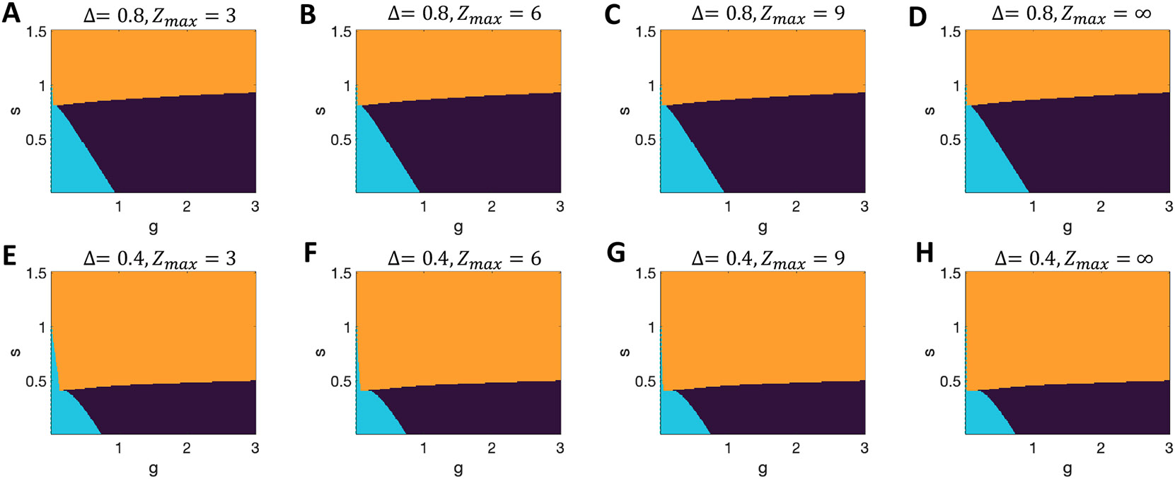
A-D. Results with with varying threshold, , for the number of standard deviations from the mean input that a unit must receive before considering a unit in the network to switch state. The mathematical limit is shown in D, while A-C indicate the multistable region growing with increased . Note that in all cases the system with on the y-axis can not be multistable for . E-H. Results for . (Black = chaos; dark blue = chaos + quiescent stable; cyan = quiescent only; yellow = quiescent + active stable state; orange = multiple active stable states; red = stable quiescent + multiple active stables states; crimson = chaos + multiple stable active states.)
In networks with the logistic response function, for , is never exactly zero. Therefore the Gaussian distribution of will always have non-zero variance for and, even if the distribution is narrow with very small variance, the distribution always retains some vanishingly small but non-zero density at the values of required to support multiple solutions of if . However, if bifurcation points in require levels of the Gaussian-distributed that are many standard deviations from its mean of zero, such solutions give exponentially small probability of multistability in a finite network, so are unlikely to be observed in practice. Therefore, we set a threshold, , in terms of the number, , of standard deviations, , of the distribution of inputs, , such that if both bifurcation points, , are beyond the threshold ( or ) we ignore both the extra solutions and any instability they cause. To clarify the result of such a limit, we show results with multiple values of in Figure 13 (for logisitic response functions) and Figure 14 (for tanh response functions), while using a default value of in other figures. In this manner, we have used the results for an infinite system in which correlations are absent, but applied them to a system in which the number of units could range from 103 to 106 to 1015 (as changes from 3 to 6 to 9) and the results be accurate for 999 networks in 1000 of that size. For further explanation see also the text in Section 3.1.
Figure 14. Impact of the criterion for multistability in networks with tanh units.
A-D. Results with with varying threshold, , for the number of standard deviations from the mean input that a unit must receive before considering a unit in the network to switch state. The mathematical limit is shown in D, which in this case is minimally different from the results with lower in (A-C). Note that in all cases the system with on the y-axis can not be multistable for . E-H. Equivalent results for , with a tiny, but observable dependence on . (Black = chaos; cyan = quiescent only; orange = multiple active stable states.)
Footnotes
Code Availability
MATLAB codes used to produce the results in this paper are available for public download at https://github.com/primon23/Multistability-Paper.
References
- Abeles M, Bergman H, Gat I, Meilijson I, Seidemann E, Tishby N, & Vaadia E (1995). Cortical activity flips among quasi-stationary states. Proc Natl Acad Sci U S A, 92(19), 8616–8620. [DOI] [PMC free article] [PubMed] [Google Scholar]
- Ahmadian Y, Fumarola F, & Miller KD (2015). Properties of networks with partially structured and partially random connectivity. Phys Rev E Stat Nonlin Soft Matter Phys, 91(1), 012820. 10.1103/PhysRevE.91.012820 [DOI] [PMC free article] [PubMed] [Google Scholar]
- Amit DJ, Gutfreund H, & Sompolinsky H (1985a). Spin-glass models of neural networks. Phys Rev A Gen Phys, 32(2), 1007–1018. 10.1103/physreva.32.1007 [DOI] [PubMed] [Google Scholar]
- Amit DJ, Gutfreund H, & Sompolinsky H (1985b). Storing infinite numbers of patterns in a spin-glass model of neural networks. Phys. Rev. Lett, 55, 1530–1531. [DOI] [PubMed] [Google Scholar]
- Anishchenko A, & Treves A (2006). Autoassociative memory retrieval and spontaneous activity bumps in small-world networks of integrate-and-fire neurons. J Physiol Paris, 100(4), 225–236. 10.1016/j.jphysparis.2007.01.004 [DOI] [PubMed] [Google Scholar]
- Ballintyn B, Shlaer B, & Miller P (2019). Spatiotemporal discrimination in attractor networks with short-term synaptic plasticity. J Comput Neurosci, 46(3), 279–297. 10.1007/s10827-019-00717-5 [DOI] [PMC free article] [PubMed] [Google Scholar]
- Battaglia FP, & Treves A (1998). Stable and rapid recurrent processing in realistic autoassociative memories. Neural Comput, 10(2), 431–450. http://www.ncbi.nlm.nih.gov/pubmed/9472489 [DOI] [PubMed] [Google Scholar]
- Benozzo D, La Camera G, & Genovesio A (2021). Slower prefrontal metastable dynamics during deliberation predicts error trials in a distance discrimination task. Cell Rep, 35(1), 108934. 10.1016/j.celrep.2021.108934 [DOI] [PMC free article] [PubMed] [Google Scholar]
- Boboeva V, Pezzotta A, & Clopath C (2021). Free recall scaling laws and short-term memory effects in a latching attractor network. Proc Natl Acad Sci U S A, 118(49). 10.1073/pnas.2026092118 [DOI] [PMC free article] [PubMed] [Google Scholar]
- Bourjaily MA, & Miller P (2011). Excitatory, inhibitory, and structural plasticity produce correlated connectivity in random networks trained to solve paired-stimulus tasks. Frontiers in Computational Neuroscience, 5, 37. 10.3389/fncom.2011.00037 [DOI] [PMC free article] [PubMed] [Google Scholar]
- Brunel N. (2003). Dynamics and plasticity of stimulus-selective persistent activity in cortical network models. Cereb Cortex, 13(11), 1151–1161. http://www.ncbi.nlm.nih.gov/entrez/query.fcgi?cmd=Retrieve&db=PubMed&dopt=Citation&list_uids=14576207 [DOI] [PubMed] [Google Scholar]
- Cabana T, & Touboul JD (2018). Large deviations for randomly connected neural networks: II. State-dependent interactions. Advances in applied probability, 50(3), 983–1004. [Google Scholar]
- Chen B, & Miller P (2020). Attractor-state itinerancy in neural circuits with synaptic depression. J Math Neurosci, 10(1), 15. 10.1186/s13408-020-00093-w [DOI] [PMC free article] [PubMed] [Google Scholar]
- Daelli V, & Treves A (2010). Neural attractor dynamics in object recognition. Exp Brain Res, 203(2), 241–248. 10.1007/s00221-010-2243-1 [DOI] [PubMed] [Google Scholar]
- David HA, & Nagaraja HN (2003). Order Statistics (3rd ed.). John Wiley and Sons. https://doi.org/ 10.1002/0471722162 [DOI] [Google Scholar]
- Escola S, Fontanini A, Katz D, & Paninski L (2011). Hidden Markov models for the stimulus-response relationships of multistate neural systems. Neural Comput, 23(5), 1071–1132. 10.1162/NECO_a_00118 [DOI] [PubMed] [Google Scholar]
- Folli V, Leonetti M, & Ruocco G (2016). On the Maximum Storage Capacity of the Hopfield Model. Front Comput Neurosci, 10, 144. 10.3389/fncom.2016.00144 [DOI] [PMC free article] [PubMed] [Google Scholar]
- Fuster JM (1973). Unit activity in prefrontal cortex during delayed-response performance: neuronal correlates of transient memory. Journal of Neurophysiology, 36(1), 61–78. 10.1152/jn.1973.36.1.61 [DOI] [PubMed] [Google Scholar]
- Goldberg JA, Rokni U, & Sompolinsky H (2004). Patterns of ongoing activity and the functional architecture of the primary visual cortex. Neuron, 42(3), 489–500. http://www.ncbi.nlm.nih.gov/pubmed/15134644 [DOI] [PubMed] [Google Scholar]
- Golos M, Jirsa V, & Dauce E (2015). Multistability in Large Scale Models of Brain Activity. PLoS Comput Biol, 11(12), e1004644. 10.1371/journal.pcbi.1004644 [DOI] [PMC free article] [PubMed] [Google Scholar]
- Hebb DO (1949). The organization of behavior; a neuropsychological theory. Wiley. [Google Scholar]
- Hopfield JJ (1982). Neural networks and physical systems with emergent collective computational abilities. Proceedings of the National Academy of Sciences, 79(8), 2554–2558. 10.1073/pnas.79.8.2554 [DOI] [PMC free article] [PubMed] [Google Scholar]
- Hopfield JJ (1984). Neurons with graded response have collective computational properties like those of two-state neurons. Proc. Natl. Acad. Sci. U.S.A, 81, 3088–3092. [DOI] [PMC free article] [PubMed] [Google Scholar]
- Jones LM, Fontanini A, Sadacca BF, Miller P, & Katz DB (2007). Natural stimuli evoke dynamic sequences of states in sensory cortical ensembles. Proc Natl Acad Sci U S A, 104(47), 18772–18777. 10.1073/pnas.0705546104 [DOI] [PMC free article] [PubMed] [Google Scholar]
- Ksander J, Katz DB, & Miller P (2021). A model of naturalistic decision making in preference tests. PLoS Comput Biol, 17(9), e1009012. 10.1371/journal.pcbi.1009012 [DOI] [PMC free article] [PubMed] [Google Scholar]
- La Camera G, Fontanini A, & Mazzucato L (2019). Cortical computations via metastable activity. Curr Opin Neurobiol, 58, 37–45. 10.1016/j.conb.2019.06.007 [DOI] [PMC free article] [PubMed] [Google Scholar]
- Lerner I, Bentin S, & Shriki O (2012). Spreading activation in an attractor network with latching dynamics: automatic semantic priming revisited. Cognitive science, 36(8), 1339–1382. 10.1111/cogs.12007 [DOI] [PMC free article] [PubMed] [Google Scholar]
- Lerner I, Bentin S, & Shriki O (2014). Integrating the automatic and the controlled: strategies in semantic priming in an attractor network with latching dynamics. Cognitive science, 38(8), 1562–1603. 10.1111/cogs.12133 [DOI] [PMC free article] [PubMed] [Google Scholar]
- Lerner I, & Shriki O (2014). Internally- and externally-driven network transitions as a basis for automatic and strategic processes in semantic priming: theory and experimental validation. Frontiers in psychology, 5, 314. 10.3389/fpsyg.2014.00314 [DOI] [PMC free article] [PubMed] [Google Scholar]
- Linkerhand M, & Gros C (2013). Generating functionals for autonomous latching dynamics in attractor relict networks. Sci Rep, 3, 2042. 10.1038/srep02042 [DOI] [PMC free article] [PubMed] [Google Scholar]
- Mazzucato L, Fontanini A, & La Camera G (2015). Dynamics of multistable states during ongoing and evoked cortical activity. J Neurosci, 35(21), 8214–8231. 10.1523/JNEUROSCI.4819-14.2015 [DOI] [PMC free article] [PubMed] [Google Scholar]
- Mazzucato L, La Camera G, & Fontanini A (2019). Expectation-induced modulation of metastable activity underlies faster coding of sensory stimuli. Nat Neurosci, 22(5), 787–796. 10.1038/s41593-019-0364-9 [DOI] [PMC free article] [PubMed] [Google Scholar]
- Miller P. (2013). Stimulus number, duration and intensity encoding in randomly connected attractor networks with synaptic depression. Front Comput Neurosci, 7, 59. 10.3389/fncom.2013.00059 [DOI] [PMC free article] [PubMed] [Google Scholar]
- Miller P. (2016). Itinerancy between attractor states in neural systems. Curr Opin Neurobiol, 40, 14–22. 10.1016/j.conb.2016.05.005 [DOI] [PMC free article] [PubMed] [Google Scholar]
- Miller P, & Katz DB (2010). Stochastic Transitions between Neural States in Taste Processing and Decision-Making. The Journal of Neuroscience, 30(7), 2559–2570. 10.1523/jneurosci.3047-09.2010 [DOI] [PMC free article] [PubMed] [Google Scholar]
- Miller P, & Katz DB (2011). Stochastic Transitions between States of Neural Activity. In Ding M & Glanzman DL (Eds.), The Dynamic Brain: An Exploration of Neuronal Variability and Its Functional Significance (pp. 29–46). Oxford University Press. [Google Scholar]
- Mitzenmacher M. (2004). A brief history of generative models for power law and lognormal distributions. Internet Mathematics, 1(2), 226–251. [Google Scholar]
- Morcos AS, & Harvey CD (2016). History-dependent variability in population dynamics during evidence accumulation in cortex. Nat Neurosci, 19(12), 1672–1681. 10.1038/nn.4403 [DOI] [PMC free article] [PubMed] [Google Scholar]
- Moreno-Bote R, Rinzel J, & Rubin N (2007). Noise-induced alternations in an attractor network model of perceptual bistability. J Neurophysiol, 98(3), 1125–1139. 10.1152/jn.00116.2007 [DOI] [PMC free article] [PubMed] [Google Scholar]
- Perin R, Berger TK, & Markram H (2011). A synaptic organizing principle for cortical neuronal groups. Proc Natl Acad Sci U S A, 108(13), 5419–5424. https://doi.org/1016051108 [pii] 10.1073/pnas.1016051108 [DOI] [PMC free article] [PubMed] [Google Scholar]
- Perline R. (2005). Strong, Weak and False Inverse Power Laws. Statistical Science, 20(1), 68–88. [Google Scholar]
- Ponce-Alvarez A, Nacher V, Luna R, Riehle A, & Romo R (2012). Dynamics of cortical neuronal ensembles transit from decision making to storage for later report. The Journal of neuroscience : the official journal of the Society for Neuroscience, 32(35), 11956–11969. 10.1523/JNEUROSCI.6176-11.2012 [DOI] [PMC free article] [PubMed] [Google Scholar]
- Rabinovich M, Volkovskii A, Lecanda P, Huerta R, Abarbanel HD, & Laurent G (2001). Dynamical encoding by networks of competing neuron groups: winnerless competition [Research Support, Non-U.S. Gov't Research Support, U.S. Gov't, Non-P.H.S.]. Physical Review Letters, 87(6), 068102. http://www.ncbi.nlm.nih.gov/pubmed/11497865 [DOI] [PubMed] [Google Scholar]
- Rabinovich MI, Varona P, Tristan I, & Afraimovich VS (2014). Chunking dynamics: heteroclinics in mind. Front Comput Neurosci, 8, 22. 10.3389/fncom.2014.00022 [DOI] [PMC free article] [PubMed] [Google Scholar]
- Rainer G, & Miller EK (2000). Neural ensemble states in prefrontal cortex identified using a hidden Markov model with a modified EM algorithm. Neurocomputing, 32, 961–966. https://doi.org/Doi 10.1016/S0925-2312(00)00266-6 [DOI] [Google Scholar]
- Rajan K, & Abbott LF (2006). Eigenvalue spectra of random matrices for neural networks. Phys Rev Lett, 97(18), 188104. http://www.ncbi.nlm.nih.gov/pubmed/17155583 [DOI] [PubMed] [Google Scholar]
- Recanatesis S, Pereira U, Murakami M, Mainen Z, & Mazzucato L (2022). Metastable attractors explain the variable timing of stable behavioral action sequences. Neuron. [DOI] [PMC free article] [PubMed] [Google Scholar]
- Russo E, & Treves A (2012). Cortical free-association dynamics: distinct phases of a latching network. Phys Rev E Stat Nonlin Soft Matter Phys, 85(5 Pt 1), 051920. 10.1103/PhysRevE.85.051920 [DOI] [PubMed] [Google Scholar]
- Sadacca BF, Mukherjee N, Vladusich T, Li JX, Katz DB, & Miller P (2016). The Behavioral Relevance of Cortical Neural Ensemble Responses Emerges Suddenly. The Journal of Neuroscience, 36(3), 655–669. 10.1523/jneurosci.2265-15.2016 [DOI] [PMC free article] [PubMed] [Google Scholar]
- Seidemann E, Meilijson I, Abeles M, Bergman H, & Vaadia E (1996). Simultaneously recorded single units in the frontal cortex go through sequences of discrete and stable states in monkeys performing a delayed localization task. J Neurosci, 16(2), 752–768. http://www.ncbi.nlm.nih.gov/pubmed/8551358 [DOI] [PMC free article] [PubMed] [Google Scholar]
- Sompolinsky H, & Crisanti A (2018). Path integral approach to random neural networks. Physical Review E, 98, 062120. [Google Scholar]
- Sompolinsky H, Crisanti A, & Sommers HJ (1988). Chaos in random neural networks. Phys Rev Lett, 61(3), 259–262. 10.1103/PhysRevLett.61.259 [DOI] [PubMed] [Google Scholar]
- Sompolinsky H, & Kanter II (1986). Temporal association in asymmetric neural networks. Phys Rev Lett, 57(22), 2861–2864. 10.1103/PhysRevLett.57.2861 [DOI] [PubMed] [Google Scholar]
- Song S, Sjöström PJ, Reigl M, Nelson S, & Chklovskii DB (2005). Highly nonrandom features of synaptic connectivity in local cortical circuits. PLoS Biol, 3(3), e68. https://doi.org/04-PLBI-RA-0489R2 [pii] 10.1371/journal.pbio.0030068 [DOI] [PMC free article] [PubMed] [Google Scholar]
- Song S, Yao H, & Treves A (2014). A modular latching chain. Cogn Neurodyn, 8(1), 37–46. 10.1007/s11571-013-9261-1 [DOI] [PMC free article] [PubMed] [Google Scholar]
- Stepanyants A, & Chklovskii DB (2005). Neurogeometry and potential synaptic connectivity. Trends Neurosci, 28, 387–394. [DOI] [PubMed] [Google Scholar]
- Stern M, Sompolinsky H, & Abbott LF (2014). Dynamics of random neural networks with bistable units. Physical review. E, Statistical, nonlinear, and soft matter physics, 90(6), 062710–062710. 10.1103/PhysRevE.90.062710 [DOI] [PMC free article] [PubMed] [Google Scholar]
- Strogatz SH (2015). Nonlinear Dynamics and Chaos (2nd ed.). Westview Press. [Google Scholar]
- Taylor JD, Chauhan AS, Taylor JT, Shilnikov AL, & Nogaret A (2022). Noise-activated barrier crossing in multiattractor dissipative neural networks. Phys Rev E, 105(6–1), 064203. 10.1103/PhysRevE.105.064203 [DOI] [PubMed] [Google Scholar]
- Touboul JD, & Ermentrout GB (2011). Finite-size and correlation-induced effects in mean-field dynamics. J Comput Neurosci, 31(3), 453–484. 10.1007/s10827-011-0320-5 [DOI] [PubMed] [Google Scholar]
- Treves A. (1990). Graded-response neurons and information encodings in autoassociative memories. Phys Rev A, 42(4), 2418–2430. http://www.ncbi.nlm.nih.gov/pubmed/9904294 [DOI] [PubMed] [Google Scholar]
- Treves A. (2005). Frontal latching networks: a possible neural basis for infinite recursion. Cogn Neuropsychol, 22(3), 276–291. 10.1080/02643290442000329 [DOI] [PubMed] [Google Scholar]
- Wills TJ, Lever C, Cacucci F, Burgess N, & O'Keefe J (2005). Attractor Dynamics in the Hippocampal Representation of the Local Environment. Science, 308(5723), 873–876. https://doi.org/doi: 10.1126/science.1108905 [DOI] [PMC free article] [PubMed] [Google Scholar]
- Wilson H, & Cowan J (1973). A Mathematical Theory of the Functional Dynamics of Cortical and Thalamic Nervous Tissue. Kybernetik, 13, 55–80. 10.1007/BF00288786 [DOI] [PubMed] [Google Scholar]
- Zurada JM, Cloete I, & van der Poel E (1996). Generalized Hopfield networks for associative memories with multi-valued stable states. Neurocomputing, 13, 135–149. [Google Scholar]