Watershed: a more efficient sampling unit for mountain camera traps

Abstract

Wildlife camera trap (CT) surveys typically employ two-dimensional equal-area grid sampling, which often neglects the influence of complex mountainous terrain on species distribution, potentially yielding misleading outcomes. A watershed, incorporating diverse habitats from high to low elevations and from rivers to ridges, aligns with complex mountains. Monitoring based on watersheds might address this. In southwest China’s mountain forests, under comparable sampling intensities, we contrasted the capture rate (CR), species richness, and relative abundance index (RAI) of dominant species among watershed, 1 × 1 km² grid, and elevation gradient patterns. Also, habitat factor correlations and heterogeneities were analyzed. Results reveal higher CR, species richness, and habitat heterogeneity in the watershed pattern. The elevation gradient pattern shows more stable species and RAI than the grid pattern. In small-scale mountains, topographic factors indirectly affect CT survey results via vegetation distribution. Analysis of similarities (ANOSIM) indicates significant differences in species and community among watersheds. Using watersheds as sampling units for CTs can match the mountains’ elevation differences and complex topography well, aids in capturing wildlife diversity and understanding mountain species distribution. Therefore, we recommend that the spatial sample design in mountainous areas should be based on watersheds, taking elevation gradients and topography into consideration.

Supplementary Information

The online version contains supplementary material available at 10.1038/s41598-025-86031-w.

Introduction

Wildlife, an essential biological group in ecosystem research and conservation management and of critical significance for human sustainable development, is under pressure due to severe human-induced disruptions and global climate change^1,2. Thus, monitoring wildlife populations and their diversity is of utmost importance. Surveys and long-term monitoring can provide a reference for understanding the evolution and trajectories of biodiversity and guidance for the conservation and exploitation of natural resources^3,4. Rapid and accurate surveys that minimize the consumption of resources such as manpower, materials and time to a large degree in a region depend on proper survey design, like sampling methods⁵. The spatial design of sampling can influence the species and magnitude of detected changes and processes⁶. Mountain areas host a substantial proportion of the world’s species due to their special topographic, geology and climatic factors^7,8, while it is vulnerable to human interaction and other climate change⁹. Therefore, exploring efficient methods for biodiversity monitoring and surveys in those areas is particularly important⁶. The spatial design used commonly in ecology, such as regular grids or lattices, was also used in mountain ecosystem diversity surveys. However, such a design might be inefficient and even misleading for the following reasons.

Elevation and complex topography shape species distribution patterns in mountain ecosystems¹⁰, which might be neglected in a random or grid spacing design¹¹, which is an artificial division. It is proven that a sampling considering elevation significantly impacts species distribution assessment¹². Furthermore, the gullies in the mountains and the ridges that connect them create intricate and varied surfaces that increase the area and shape of varied microhabitats¹³. The ridges and rivers can also limit the dispersion of species, leading to specific community distribution patterns¹⁴. In summary, the topographically complex must be considered in sampling in montane ecosystems. A good sampling unit should be consistent with the distribution patterns of species resulting from natural processes related to resources, species movement and human activities. It is unreasonable to infer species status and distribution patterns in topographically complex instead based on data obtained from two-dimensional spatial sampling designs¹⁵.

The watershed is a region that is “closed”, physically defined by a water divide, which is basic outline constructed by the Earth’s internal forces and modified by external forces¹⁶. A watershed unit can encompass different habitat types and ecosystems from high to low elevations and from river to ridge. The ecosystems connected by river form the basic spatial ecological unit within which terrestrial ecosystems operate^17,18. At the same time, the species composition within a watershed unit is relatively stable because rivers and watersheds constrain movement of many species^19–21. Using the watershed as the unit of ecological study provides a theoretically clearer and more realistic picture of ecosystem functions and services¹⁶.

Camera traps (CTs) are increasingly used for monitoring wildlife diversity because they are continuous, efficient, non-invasive and repeatable^22–24. The study on the influence on survey efficiency of camera type²⁵, trigger interval setting²⁶, number and placement²⁷, camera days and spacing²⁸ have been discussed, which have promoted the standardization of CTs operations. In terms of spacing sampling, most previous surveys also apply grids of equal size (usually 1 × 1 km²)^29,30. Whether systematic sampling using watersheds as sampling units for CTs can improve survey efficiency and obtain representative data in mountainous regions has not yet been attempted.

Based on this, we conducted an experiment in the Shibaoshan ecotourism area (SBS) in southwest China. We surveyed ground bird and mammal diversity using watershed, grid and elevation-based designs and compared the results. This study attempts to apply the disciplinary concept of watershed ecology from the theoretical level to practical biological conservation. It provides a reference for the determination of CTs sampling units and the design of sampling patterns in mountainous regions, which is essential for the conservation and management of ecosystems.

Methods

Study area

This study was conducted in the SBS (99°48′—99°52′ E, 26°22′—26°25′ N; elevation range: 1900–3000 m; area of about 20 km²) in Jianchuan County, Dali Bai Autonomous Prefecture, Yunnan Province, China (Fig. 1). The area is a Danxia landform, a branch of the southward extension of the Laojun Mountain Range, a World Natural Heritage Site. It is part of the Lancang River system. The climate is a southern temperate plateau-type monsoon climate, with an average annual temperature of 7–21 °C and an average annual precipitation of 572.7 mm. The climate is circular and three-dimensional, influenced by the elevation difference and topography. The particular climate has given rise to a wealth of wildlife resources in the region. The main vegetation types are cold-temperate coniferous forest, deciduous broad-leaved forest, and evergreen broad-leaved forest. The dominant tree species is mainly Yunnan pine, with evergreen broad-leaved forests in the gullies and valleys, mainly in the family Fagaceae.

Fig. 1.

Camera trap placement, (A) shows all - camera - trap placement, (B) shows watershed - pattern placement. We measured the area of each watershed unit, and selected four watershed units that accounted for more than 10% of the total area for camera deployment.

Camera placement

In the SBS, the area with an elevation < 2400 m is predominantly used for human development, encompassing towns, villages, agricultural fields, roads, tourism sites, and other forms of land use. Consequently, our research area was designated within the forested region at an elevation range of 2400–2900 m, where human disturbances are relatively minimal. During the sampling design process, we formulated the sampling schemes for the watershed pattern, the 1 × 1 km² grid pattern, and the elevation gradient pattern. The specific details are as follows:

1. Watershed pattern: We obtained a topographic map of the study area from satellite imagery and delineated the watersheds and their boundaries. Eight watersheds were identified, numbered A to H (Fig. 1B). We hypothesized that a larger watershed unit would exhibit a higher level of species diversity. By selecting for larger watershed units in our investigation, we could curtail the input costs associated with sampling, including the quantity of camera traps (CTs), human resources, and time expenditure, thereby facilitating an efficient assessment of the species diversity within the target area. Therefore, we measured the area of each watershed unit, and selected 4 watershed units that accounted for more than 10% of the total area for camera deployment (Table 1).

Table 1.

Area percentage of different watershed units and the number of camera traps deployed.

Watershed no.	Area (km2)	Percentage (%)	Number of camera traps
			Planned	Actual
A	3.527	29.35%	5	3
B	3.289	27.37%	5	5
C	1.947	16.20%	4	4
D	1.614	13.43%	4	4
E	0.921	7.66%	0	0
F	0.383	3.19%	0	0
G	0.216	1.80%	0	0
H	0.153	1.27%	0	0

The deployment of CTs within the watersheds was carried out in accordance with the following rules: CTs were placed from the estuary of the main stream to the highest point of the selected watershed. To account for the diverse terrains on both sides of the main stream within the watershed, we alternately selected a main tributary on either side of the main stream every 100 m of vertical elevation for CT deployment. If the elevation span of the tributary was < 200 m, a CT was placed only near the intersection of the tributary and the major stream or around the center point of the tributary. If the elevation span was > 200 m, in addition to placing a CT at the intersection of the tributary and the main stream, additional CTs were placed every 100 m of elevation along the tributary upward (Fig. 2).

Fig. 2.

Schematic of camera traps sampling design in watershed unit.

We planned to deploy 4 CTs in the watersheds with an area proportion ranging from 10 to 20% (approximately 1.2–2.4 km²). Five CTs in the watersheds with an area proportion from 20 to 30% (with an area of approximately 2.4–3.6 km²). Owing to logistical constraints, two preset CTs in Watershed A within the watershed pattern could not be accomplished. Consequently, only 3 CTs were installed in this particular watershed unit. Across the 4 selected watershed units, we managed to set up 16 CTs in total (Table 1; Fig. 1B).

• (2)1 × 1 km² grid pattern: We divided the research area into several 1 × 1 km² grids, and preset at least one CT in each grid.
• (3)Elevation gradient pattern: A CT was preset within every 100-meter elevation interval on one side of the main mountain within the research area, and CTs were deployed on the other side in the same way. For simplicity, hereinafter “grid pattern” is used to denote the “1 × 1 km² grid pattern”, and “elevation pattern” is used to represent the “elevation gradient pattern”.

We integrated the sampling designs of the watershed pattern, the 1 × 1 km² grid pattern and the elevation gradient pattern. From 7 to 9 January, 2022, we deployed 27 CTs. We installed cameras on tree trunks between 0.5 and 1.5 m in height and prioritized wildlife trails, water points, feeding points. The camera type we used was CL-S1 (Qingdao Yequziran Technology Co., LTD). We set the camera mode to record 20s of video after taking two consecutive pictures, the trigger interval to 0s and the sensitivity to ‘medium’. We recorded the longitude, latitude and elevation of each CT, and in detail documented the proportion of vegetation types (including Yunnan pine forest, evergreen broad-leaved forest, shrubland and herbaceous plants) within a 100 m² area centered around each CT. We recovered all the CTs from 1 to 3 April 2022, and they were in operation for 3 months, during which time they were serviced once.

Environmental data

To further explore the impacts of different habitat factors on the species monitoring results of CTs and the differences in habitats covered by different sampling patterns, we extracted the slope and aspect of each CT using QGIS 3.28 software. For the convenience of analysis, we assigned values to aspects from north to south as follows: north (0° – 22.5° and 337.5° − 360°) was assigned a value of 1; northeast (22.5° − 67.5°) and northwest (292.5° − 337.5°) were 1.5; east (67.5° − 112.5°) and west (247.5° − 337.5°) were 2; southeast (112.5° − 157.5°) and southwest (202.5° − 247.5°) were 1.5; south (157.5° − 202.5°) was 3. We also calculated the topographic distances between each CT and the nearest residential areas and water sources. We used the Normalized Difference Vegetation Index (NDVI) as the net primary productivity index. The NDVI of each CT was extracted based on an existing database, which was calculated using Landsat 5/7/8/9 images on the Google Earth Engine cloud computing platform with a resolution of 30 × 30 m^31,32.

Data resampling comparison

In order to ensure that the watershed pattern has the same number of CTs as the grid pattern and the elevation pattern, to ensure the comparability of the data, we resampled the data of the 1 × 1 km² grid pattern and the Elevation pattern ten times. The specific operation process is as follows:

1. 1 × 1 km² grid pattern: We imported the geographic coordinates of the 27 CTs into QGIS 3.28 software. We generated one random point in the range of 99°49′30″—99°51′30″E, 26°22′00″—26°25′00″N. Sixteen 1 × 1 km² grids were generated with the random point as the center, ensuring at least one CT distribution in each grid. If there is no CTs distribution in a grid, the random point and grid are regenerated. If more than one camera exists in a grid, one of them is randomly selected. Repeat the sampling ten times.

2. Elevation gradient pattern: We stratified the sampling based on the elevation distribution interval of all CTs and took 16 CTs as data for the elevation pattern, repeating the sampling ten times (Table 2).

Table 2.

Resampling of camera traps for elevation pattern.

Elevation gradients	Number of camera traps
	Total	Elevation pattern
2400–2499 m	5	3
2500–2599 m	5	3
2600–2699 m	7	4
2700–2799 m	5	3
2800–2900 m	5	3

Data analysis

The data collected were processed using the software CTIMCS³³. The videos taken were used to aid in species identification. We referred to relevant books for species identification^34–37 and specification of species names^38,39. Species that could not be accurately identified, such as small nocturnal rodents and bats, were excluded from the analysis.

Each camera working continuously for 24 h was considered a camera day. Different individuals or species captured (based on stripes, fur color, body shape, gender, and age class) at the same station within 30 min were defined as independent photographs (IP). When individuals could not be identified, consecutive individuals or species captured at the same station at least 30 min intervals were considered IP⁴⁰.

We estimated and compared the species richness of the three sampling patterns using rarefaction curves and estimated confidence intervals using the bootstrap method⁴¹. The calculations associated with the sparsely drawn curves were done in the R statistical programming environment using the “iNEXT” package⁴².

We calculated the Capture Rate (CR) for the three sampling patterns to compare the monitoring efficiency⁴³, defined as follows:

1

where N is the number of IP obtained for each sampling pattern (per sample), T is the number of camera days for each sampling pattern.

We computed Relative Abundance Index (RAI) to assess the relative population size of the species obtained from the three sampling patterns⁴⁰, defined as follows:

2

where A_i represents the number of IP of animals of i (i = 1, 2, ...), T is the number of camera days for each sampling pattern.

There are certain differences in the habitats covered by different sampling patterns, and this will have an impact on the monitoring results. In view of this, we further analyzed the correlation between habitat factors and survey results in depth, and analyzed the habitat heterogeneity under different sampling patterns by means of weighting.

Firstly, we standardized the habitat factors of all CTs and the wildlife monitoring results (including the number of species, the capture rate and the RAI of dominant species) to make their mean values reach 0 and standard deviations reach 1. Subsequently, we used the Spearman’s rank correlation test method to analyze the correlation among various habitat factors as well as the correlation between habitat factors and wildlife monitoring results, and set the significance level at p < 0.05.

When calculating the habitat heterogeneity covered by different sampling patterns, we determined the correlation weight (wi) of each habitat factor in wildlife monitoring based on the absolute value of the correlation coefficient (rEi) between different standardized habitat factors (Ei) of each camera trap and the wildlife monitoring results. The formula is as follows:

3

where w_i represents the relative weight of the i-th habitat factor for wildlife monitoring, and m represents the total number of wildlife monitoring results. r_Eik represents the correlation coefficient between the i-th habitat factor (Ei) and the k-th wildlife monitoring result. n represents the total number of habitat factors, and r_Ejk represents the sum of the absolute values of the correlation coefficients between the j-th habitat factor and the m wildlife monitoring results.

Next, the habitat factors of a single CT were weighted and accumulated to obtain the comprehensive habitat index (I_k). Finally, the mean value and standard deviation (I_σ) of the comprehensive index for each sampling pattern were calculated, and I_σ was used to reflect the differences in habitat heterogeneity among different sampling patterns.

4

5

6

In the formula, I_k represents the comprehensive index of the habitat factors of the k-th camera trap (CT), and E_ik represents the value of the i-th habitat factor of the k-th CT. is the average comprehensive index of a certain sampling pattern, and m is the number of CTs in a certain sampling pattern. is the standard deviation of the comprehensive index of the habitat factors of a certain sampling pattern, which represents the habitat heterogeneity covered by different sampling patterns. The higher its value is, the greater the habitat heterogeneity will be.

We used Analysis of Similarities (ANOSIM) to compare differences in communities (birds and mammals) between and within watersheds. We calculated the mean rank of similarity between (r_B) and within (r_W) watersheds separately using the RAI of each species monitored by each CT, and calculated similarity R-values (ANOSIM statistic R) using the following formula:

7

Where n is the number of all cameras⁴⁴. -1 < R < 1, if R > 0 indicates more significant community dissimilarity between watersheds and more remarkable community similarity within watersheds; if R = 0 indicates no difference in similarity between and within watersheds; and if R < 0 shows more remarkable similarity between watersheds and more significant dissimilarity within watersheds, we used a permutation test to calculate P-values to determine whether there were significant differences in community composition across watersheds, with the level of significance of differences set at P < 0.05 ⁴⁴.ANOSIM analyses were conducted in R programming software using the package “vegan”⁴².

Results

Capture rate and species richness

All 27 CTs worked effectively during the survey, accumulating 1677 camera days, and yielding 29,416 photos. Of the total number of photos captured, 7378 were of wildlife (with 1915 IP); 216 were of researchers; 1255 were of human disturbance, including villagers, domestic cattle, domestic sheep, dogs, etc.; 1986 were of unidentifiable wildlife, including small rodents and vestigial images. A total of 49 species of wildlife were identified, including 13 species of mammals belonging to 5 orders and 9 families and 36 species of birds belonging to 3 orders and 16 families (Supplementary Table S1).

The watershed pattern accumulated 1049 camera days with 1431 IP and a CR of 1.36; the grid pattern camera days were 1081 ± 18.87d (mean ± SD) with 1001.80 ± 52.58 IP and a CR of 0.99 ± 0.16; the elevation pattern camera days were 988.7 ± 22.61d with 1242.10 ± 52.61 IP and a CR of 1.26 ± 0.18 (Fig. 3). The capture rate for the watershed sampling pattern was higher than the average of the elevation and grid patterns (Fig. 3).

Fig. 3.

Capture rates of different sampling patterns, dots are the means of multiple sampling, error bars are standard deviations.

The watershed pattern yielded a species richness of 46.00 species (93.88% of all species recorded in 27 cameras), of which 33.00 were birds (91.67% of all birds recorded), and 13.00 were mammals (100%, Fig. 4, Supplementary Table S2). The grid pattern obtained a species richness of 38.20 ± 2.05 (mean ± SE), with a minimal value of 28 and a maximal value of 47, of which birds 26.20 ± 1.99 (16–34) and mammals 12.00 ± 0.15 (11–13) (Fig. 4ace, Supplementary Table S2). The elevation pattern yielded species richness of 38.30 ± 1.67 (30–43), of which birds 26.5 ± 1.53 (19–31) and mammals 12.3 ± 0.21 (11–13) (Fig. 4 bdf, Supplementary Table S2). The species richness estimated by rarefaction curves of the watershed sampling pattern is higher than the average value of grid and elevation design in both bird and mammal surveys (Fig. 4).

Fig. 4.

Rarefaction curves and species richness for the three camera trap sampling patterns, shading indicates 95% confidence intervals. (a,b) is bird and mammal; (c,d) is bird; (e,f) is mammal).

RAI of dominant species

We analyzed six species’ RAI with more than 100 IP. The Perny’s long-nosed squirrel (Dremomys pernyi) was captured with a total IP of 371 and a total RAI of 22.12; the watershed pattern surveyed with an RAI of 28.88; the grid pattern RAI was 17.87 ± 8.56 (mean ± SE); and the elevation pattern RAI was 24.13 ± 7.69 (Fig. 5). The Rhesus macaque (Macaca mulatta) was captured with a total IP of 367, and a total RAI of 21.88; the watershed pattern RAI was 22.40; the grid pattern RAI was 19.03 ± 6.92; and the elevation pattern RAI was 22.09 ± 6.03 (Fig. 5). Lady Amherst’s pheasant (Chrysolophus amherstiae) was captured with a total IP of 152 and a total RAI of 9.06; the watershed pattern RAI was 12.11; the grid pattern RAI was 8.59 ± 2.55; and the elevation pattern RAI was 10.22 ± 2.84 (Fig. 5). The Forrest’s rock squirrel (Rupestes forresti) was captured with a total IP of 122 and a total RAI of 7.27; the watershed pattern RAI was 6.58; the grid pattern RAI was RAI 5.56 ± 3.49; and the elevation pattern RAI was 9.012 ± 1.64 (Fig. 5). Northern red muntjac (Muntiacus vaginalis) was captured with a total IP of 117 and a total RAI of 6.98; the watershed pattern RAI was 8.87; the grid pattern RAI was 6.50 ± 0.84; and the elevation pattern RAI was 7.57 ± 0.62 (Fig. 5). Pallas’s squirrel (Callosciurus erythraeus) was captured with a total IP of 110 and a total RAI of 6.56; the watershed pattern RAI was 7.24; the grid pattern RAI was 6.19 ± 1.64; and the elevation pattern RAI was 6.87 ± 1.96 (Fig. 5).

Fig. 5.

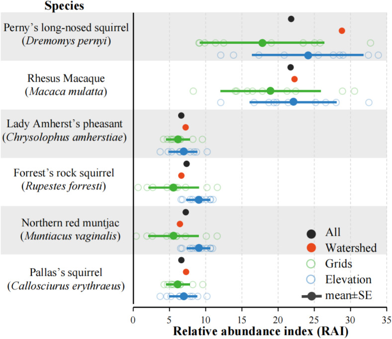
Relative abundance indices of dominant species (independent photographs > 100) for different sampling patterns.

In the watershed pattern, the RAI of five species was close to the total RAI, except for the RAI of the Perny’s long-nosed squirrel, which was high compared to the total RAI (Fig. 5). In the grid pattern, the RAI of all six dominant species was lower than the total RAI, and ten replicates showed that the RAI of the four species was dispersed, except for the Lady Amherst’s pheasant and the Pallas’s squirrel, where the RAI was more concentrated (Fig. 4). For the elevation pattern, the RAI of all six species was close to the total RAI, and the ten replicates showed that the RAI of four of these species was more concentrated, except for the Penry’s long-nosed squirrel and the Rhesus macaque (Fig. 5).

Correlation between habitat factors and CTs monitoring, and habitat heterogeneity of sampling patterns

The correlation between species number and habitat factors shows specific patterns. For topographic factors (elevation, slope, aspect), species number has no significant correlation (Fig. 6a). It has a significant positive correlation with the distance between CTs and residential areas (r = 0.52, p < 0.01), a significant negative correlation with the distance from water sources (r = 0.54, p < 0.01), and a significant positive correlation with NDVI (r = 0.39, p < 0.05) (Fig. 6a). In vegetation type proportion, species number has a significant negative correlation with Yunnan pine forest proportion (r = -0.42, p < 0.05) and a significant positive correlation with broad-leaved forest proportion (r = 0.44, p < 0.05), but no significant correlation with shrub and herbaceous plant proportions (Fig. 6a). The CR has a significant negative correlation with the distance from CTs to water sources (r = -0.58, p < 0.01), and other habitat factors have no significant correlation with CR (Fig. 6a). The RAI of Perny’s long-nosed squirrel has a significant negative correlation with the distance from CTs to water sources (r = -0.60, p < 0.01); the RAI of the Rhesus macaque has a significant negative correlation with the distance from CTs to residential areas (r = -0.57, p < 0.01); the RAI of Lady Amherst’s pheasants has a significant negative correlation with the distance from CTs to water sources (r = -0.50, p < 0.01); the RAI of Forrest’s rock squirrel has no significant correlation with any habitat factor; the RAI of the Northern red muntjac has a significant negative correlation with slope (r = -0.39, p < 0.05); the RAI of Pallas’s squirrel has a significant negative correlation with the distance from CTs to water sources (r = -0.41, p < 0.05) and a significant positive correlation with NDVI (r = 0.48, p < 0.05) (Fig. 6a).

Fig. 6.

Correlation between habitat factors and species monitoring results (a) and comparison of habitat heterogeneity under different sampling patterns (b), error bars are standard deviations).

Although topographic factors have no significant correlation with species monitoring results, elevation has a highly significant positive correlation with Yunnan pine forest proportion (r = 0.62, p < 0.001) and significant negative correlations with the proportions of broad-leaved forests (r = -0.52, p < 0.01), shrubs (r = -0.50, p < 0.01), and herbaceous plants (r = -0.47, p < 0.05) (Fig. 6a). Slope has a significant negative correlation with the proportion of herbaceous plants (r = -0.59, p < 0.01); aspect has a highly significant negative correlation with NDVI (r = -0.62, p < 0.001), a significant positive correlation with proportion of broad-leaved forests (r = 0.50, p < 0.01), and a significant negative correlation with shrub proportion (r = -0.39, p < 0.05) (Fig. 6a).

There are differences in habitat heterogeneity among sampling patterns. The watershed pattern has the highest habitat heterogeneity index () of 3.75, followed by the grid pattern (3.41 ± 0.43) and the elevation pattern (3.41 ± 0.62) (Fig. 6b). The maximum (4.31) and the minimum (2.29) of occur in the elevation pattern (Fig. 6b). Due to the existence of direct or indirect significant correlations between habitat factors and species monitoring results, as well as the differences in habitat heterogeneity indices among different sampling patterns, this indicates that the habitats covered by different sampling patterns vary greatly, which in turn leads to significant differences in monitoring results.

Community composition between watershed units

We analyzed the community composition differences between the watershed units by the watershed sampling pattern. Analysis of Similarities (ANOSIM) indicated that both bird (R = 0.369, P = 0.024) and mammal (R = 0.315, P = 0.010) community composition differed significantly between watersheds. For birds, no species were captured in all watershed units. The Lady Amherst’s pheasant was captured in Watersheds A, B and D. Three species were captured together in both Watersheds A and D, the Chestnut thrush (Turdus rubrocanus), the Chinese thrush (Turdus mupinensis) and the Eurasian jay (Garrulus glandarius). Five species were captured in both Watersheds B and D, namely the White-browed bush robin (Tarsiger indicus), the Streak-breasted scimitar babbler (Pomatorhinus ruficollis), the Black-streaked scimitar babbler (Pomatorhinus gravivox), the Moustached laughing thrush (Ianthocincla cineraceus), the White-throated fantail (Rhipidura albicollis). Nine species were captured in Watershed A only, including the Mrs. Hume’s pheasant (Syrmaticus humiae), the White-crowned forktail (Enicurus immaculatus), etc. Five species were captured only within Watershed B, including the Dark-breasted rosefinch (Procarduelis nipalensis), the Alpine thrush (Zoothera mollissima), etc. Two species were surveyed in Watershed C only, the Brown wood owl (Strix leptogrammica), and the Black-headed sibia (Heterophasia desgodinsi), Eight species were surveyed in Watershed D only, including the Blue whistling thrush (Myophonus caeruleus), the Elliot’s laughingthrush (Trochalopteron elliotii) etc. (Fig. 7a, Supplementary Table S1).

Fig. 7.

Differences in species composition captured by camera traps between the four watershed units (a bird, b mammal).

For mammals, four species were captured in all watershed units: the Masked palm civet (Paguma larvata), the Northern red muntjac, the Pallas’s squirrel, and the Perny’s long-nosed squirrel. Two species were captured in Watersheds B, C and D: the Forrest’s rock squirrel and the Yunnan porcupine (Hystrix brachyura). Two species, the Northern tree shrew (Tupaia belangeri) and the Yellow-throated marten (Martes flavigula), were captured in both Watersheds A and C. The species captured in Watersheds A and D was the Yunnan hare (Lepus comus). The species captured in Watershed A only was the wild boar (Sus scrofa); in Watershed B only was the Swinhoe’s striped squirrel (Tamiops swinhoei) and the Indian Giant flying squirrel (Petaurista philippensis); and in Watershed C only was the Rhesus macaque (Fig. 7b, Supplementary Table S1).

Discussion

In the comparative data of three sampling patterns, the elevation and grid patterns were resampled ten times. Each pattern had 16 CTs and similar camera working days, ensuring data comparability. Under the same survey intensity conditions, when the sampling design based on watershed units is applied in mountainous areas, the capture rate and species richness it generates are higher compared to the elevation or grid patterns.

In this survey, we found that there was no significant correlation between topographic factors (including elevation, aspect, and slope) and the monitoring results of CTs, and this finding differs from the results of previous studies⁴⁵. We speculate that this may be due to the relatively small spatial scale involved in this survey. However, our research results have indeed confirmed that there is a significant correlation between elevation and aspect and the proportion of vegetation types, and the vegetation types have a direct and significant correlation with the monitoring results of wild animals. This means that the complex topographic factors in mountainous areas can affect the distribution of vegetation types and thereby indirectly affect the distribution and monitoring results of wildlife.

Different species have preferences for habitat selection. The results of our survey show that the farther away from residential areas, the higher the species diversity, which strongly indicates that most wildlife will avoid human disturbances. However, the Rhesus macaque shows a preference for areas closer to residential areas, and this phenomenon is closely related to the local ecotourism activities based on macaques and the human-macaque conflicts⁴⁶. The Northern red muntjac is more sensitive to slopes and prefers to move in relatively flat areas. As different sampling patterns also have differences in the habitat heterogeneity they cover, this accounts for why the RAI of species monitored by different sampling patterns can have significant differences. Therefore, when carrying out CT surveys in mountainous areas, it is necessary to cover habitat heterogeneity as comprehensively as possible in order to obtain more representative results.

Higher habitat heterogeneity and being closer to water flows are the keys to the high efficiency of the watershed pattern. The habitat heterogeneity covered by the watershed pattern is higher than that of the grid and elevation patterns. Among them, the habitat heterogeneity index of the elevation pattern has relatively large differences during the resampling process, while the differences in the grid pattern are relatively small. This fully illustrates that in mountainous environments, the sampling pattern that considers topographic factors can cover a wider range of habitat heterogeneity. The watershed is a key element in shaping the topography of mountainous ecosystems⁴⁷. The sampling design based on the watershed can cover the mountainous habitat conditions more comprehensively and effectively take into account different topographies and habitat types. Therefore, a richer species diversity can be surveyed within a shorter period of time. In addition, our research results also confirm that the closer to the water source, the higher the number of species monitored and the CR. This is consistent with the conclusions of other previous studies^48,49. Water is a vital resource on which all species depend for their survival and growth⁵⁰. Compared with other sampling patterns, under the watershed sampling pattern, the placement positions of camera traps (CTs) may be closer to the water flow, so that the species diversity in the region can be grasped more quickly.

Our study has suggested that camera trap deployment in mountain ecosystems should consider the elevation gradient. The elevation stratified sampling pattern performed better than the grid sampling pattern regarding capture rate. At the same time, the elevation design was more stable in monitoring the species richness and RAI of dominant species than the grid arrangement. Different elevation zones in montane ecosystems include a variety of environmental conditions, which impact species richness and community composition^4,51. The planarization in the grid pattern, ensuring a uniform distribution of camera traps in two-dimensions, is suitable for plain or hilly areas with limited elevation ranges. However, in complex mountainous terrain, the grid pattern ignore the effects of vertical stratification in elevation and terrain folds on species, thus reducing the stability of the survey results.

This study still has some limitations and directions worthy of further exploration. Some of the CTs installation points selected in this survey were near wildlife paths, water sources, and foraging areas, which may have caused certain biases as these factors might increase the CR. In addition, during the analysis process, we excluded unidentifiable small rodents and bats, which might underestimate the diversity of small mammals. Although we found that the sampling based on watershed units has a high efficiency in mountain CT surveys, a standard or protocol has not been formed yet. Future studies can carry out relevant monitoring on a broader mountain scale to promote the formation of a standard. This survey shows that there are significant differences in species composition between different watershed units, especially for birds. This might be because some species are temporarily confined to specific watershed units due to the ridge isolation of watershed boundaries²⁰. Moreover, different watershed units will form unique habitat characteristics, which may also lead to differences in species richness and communities between watersheds. Therefore, we hypothesize that watersheds and rivers may be the main obstacles to species movement, and the habitat characteristics of each watershed shape different community compositions^19,52. Future studies should verify these hypotheses based on more detailed watershed surveys.

Overall, when deploying camera traps in mountainous regions, more consideration must be given to the effects of elevational vertical and complex topography on species distribution. Watersheds are a very suitable sampling unit for mountain camera trap surveys for wildlife. Species monitoring in watershed units is more than just a more efficient way of obtaining data. It can also give insight for integrating multi-taxon biogeographic studies. We suggest that future mountain camera trap monitoring should be more watershed-based and consider changes in vertical gradients in elevation.

Electronic supplementary material

Below is the link to the electronic supplementary material.

Author contributions

Conceptualization: Wen Xiao, Kun Tan, Zhi-Pang Huang; Methodology: Wen Xiao, Kun Tan, Yi-Hao Fang, Jun-Jie Li; Field data collection: Yi-Hao Fang, Jun-Jie Li, Zhi-Pang Huang, Ji-Cong Zhan, Can-Bin Huang; Data analysis: Jun-Jie Li, Xue-Jun Yang; Writing – original draft preparation: Jun-Jie Li; Writing – review and editing: All authors; Funding acquisition: Kun Tan, Yan-Peng Li, Zhi-Pang Huang, Wen Xiao, Liang-Wei Cui; Resources: Wen Xiao, Zhi-Pang Huang, Yan-Peng Li, Can-Bin Huang; Supervision: Wen Xiao, Kun Tan, Zhi-Pang Huang.

Data availability

Data is provided within the supplementary information files.

Declarations

Competing interests

The authors declare no competing interests.

References

- 1.Ripple, W. J. et al. Status and ecological effects of the world’s largest carnivores. Science 343 (2014). [DOI] [PubMed]
- 2.Ripple, W. J. et al. Collapse of the world’s largest herbivores. Sci. Adv.1 (2015). [DOI] [PMC free article] [PubMed]
- 3.Jetz, W. et al. Essential biodiversity variables for mapping and monitoring species populations. Nat. Ecol. Evol.3, 539–551 (2019). [DOI] [PubMed] [Google Scholar]
- 4.Tan, K. et al. The discontinuous elevational distribution of an ungulate at the regional scale: Implications for speciation and conservation. Animals 11 (2021). [DOI] [PMC free article] [PubMed]
- 5.Hortal, J. & Lobo, J. M. An ED-based protocol for optimal sampling of biodiversity. Biodivers. Conserv.14, 2913–2947 (2005). [Google Scholar]
- 6.De Palma, A. et al. Challenges with inferring how Land-Use affects terrestrial Biodiversity: Study Design, Time, Space and Synthesis. Adv. Ecol. Res.58, 163–199 (2018). [Google Scholar]
- 7.Antonelli, A. et al. Geological and climatic influences on mountain biodiversity. Nat. Geosci.11, 718–725 (2018). [Google Scholar]
- 8.Rahbek, C. et al. Humboldt’s enigma: what causes global patterns of mountain biodiversity? Science365, 1108–1113 (2019). [DOI] [PubMed] [Google Scholar]
- 9.Chakraborty, A. Mountains as vulnerable places: a global synthesis of changing mountain systems in the Anthropocene. GeoJournal86, 585–604 (2021). [Google Scholar]
- 10.Albrecht, J. et al. Plant and animal functional diversity drive mutualistic network assembly across an elevational gradient. Nat. Commun.9 (2018). [DOI] [PMC free article] [PubMed]
- 11.Zhang, S. S., Bao, Y. X., Wang, Y. N., Fang, P. F. & Ye, B. Comparisons of different camera trap placement patterns in monitoring mammal resources in Gutianshan National Nature Reserve. Chin. J. Ecol.31, 2016–2022 (2012). [Google Scholar]
- 12.Deng, W. et al. Sampling methods affect Nematode-Trapping Fungi biodiversity patterns across an elevational gradient. BMC Microbiol.20, 1–11 (2020). [DOI] [PMC free article] [PubMed] [Google Scholar]
- 13.Elsen, P. R., Monahan, W. B. & Merenlender, A. M. Topography and human pressure in mountain ranges alter expected species responses to climate change. Nat. Commun.11, 1–10 (2020). [DOI] [PMC free article] [PubMed] [Google Scholar]
- 14.Goldani, A., Carvalho, G. S. & Bicca-Marques, J. C. Distribution patterns of neotropical primates (Platyrrhini) based on parsimony analysis of endemicity. Braz. J. Biol.66, 61–74 (2006). [DOI] [PubMed] [Google Scholar]
- 15.Wang, J. F., Stein, A., Gao, B. B. & Ge, Y. A review of spatial sampling. Spat. Stat.2, 1–14 (2012). [Google Scholar]
- 16.Zhao, B. Watersheds are the best natural partition units for ecological studies. Sci. Technol. Rev.32, 12 (2014). [Google Scholar]
- 17.Li, X. et al. Linking Critical Zone With Watershed Science: The Example of the Heihe River Basin. Earth’s Futur. 10, eEF002966 (2022).
- 18.Wu, G. & Cai, Q. H. Expression as a whole of research content of the watershed. Acta Ecol. Sin. 18, 13–19 (1998). [Google Scholar]
- 19.Gascon, C. et al. Riverine barriers and the geographic distribution of amazonian species. Proc. Natl. Acad. Sci. U. S. A.97, 13672–13677 (2000). [DOI] [PMC free article] [PubMed] [Google Scholar]
- 20.Oliveira, U., Vasconcelos, M. F. & Santos, A. J. Biogeography of Amazon birds: Rivers limit species composition, but not areas of endemism. Sci. Rep.7, 1–11 (2017). [DOI] [PMC free article] [PubMed] [Google Scholar]
- 21.Popescu, C. et al. Riparian vegetation structure influences terrestrial invertebrate communities in an agricultural landscape. Water13 (2021).
- 22.Ahumada, J. A., Hurtado, J. & Lizcano, D. Monitoring the status and trends of tropical forest terrestrial vertebrate communities from Camera trap data: A tool for conservation. PLoS One8, 6–9 (2013). [DOI] [PMC free article] [PubMed] [Google Scholar]
- 23.Burton, A. C. et al. Wildlife camera trapping: a review and recommendations for linking surveys to ecological processes. J. Appl. Ecol.52, 675–685 (2015). [Google Scholar]
- 24.Li, S. et al. Retreat of large carnivores across the giant panda distribution range. Nat. Ecol. Evol.4, 1327–1331 (2020). [DOI] [PubMed] [Google Scholar]
- 25.Meek, P. D. et al. Recommended guiding principles for reporting on camera trapping research. Biodivers. Conserv.23, 2321–2343 (2014). [Google Scholar]
- 26.Hamel, S. et al. Towards good practice guidance in using camera-traps in ecology: influence of sampling design on validity of ecological inferences. Methods Ecol. Evol.4, 105–113 (2013). [Google Scholar]
- 27.Hofmeester, T. R. et al. Effects of camera-trap placement and number on detection of members of a mammalian assemblage. Ecosphere 12 (2021).
- 28.Colyn, R. B., Radloff, F. G. T. & O’Riain, M. J. Camera trapping mammals in the scrubland’s of the Cape Floristic Kingdom—the importance of effort, spacing and trap placement. Biodivers. Conserv.27, 503–520 (2018). [Google Scholar]
- 29.Xiao, Z. S. et al. Developing camera-trapping protocols for wildlife monitoring in Chinese forests. Biodivers. Sci.22, 704–711 (2014). [Google Scholar]
- 30.TEAMNetwork. Terrestrial Vertebrate (Camera Trap) Protocol Implementation Manual, v. 3.0. Tropical Ecology, Assessment and Monitoring Network, Center for Applied Biodiversity Science, Conservation International, Arlington, VA, USA.. https://s3images.coroflot.com/user_files/individual_files/255900_3wDuxVwoOstvJZcVSht6oYmCK.pdf (2008).
- 31.Dong, J., Zhou, Y., You, N. & Chen, C. A 30-m Annual Maximum NDVI Dataset in China from 2000 to 2022. 10.12199/nesdc.ecodb.rs.2021.012 (2023).
- 32.Yang, J. et al. Remote sensing of environment divergent shifts in peak photosynthesis timing of temperate and alpine grasslands in China. Remote Sens. Environ.233, 111395 (2019). [Google Scholar]
- 33.Yang, D. Q., Ren, G. P. & Yang, T. Camera trap images manual classification. System 1.1. https://www.eastern-himalaya.com.cn/contents/3/990.html (2019).
- 34.Yang, L. The Avifauna of Yunnan, China (Yunnan Science and Technology, 2004).
- 35.China Wildlife Conservation Association. Atlas of Mammals of China (Henan Science and Technology, 2005).
- 36.Smith, A. T. & Xie, Y. A Guide to the Mammals of China. Hunan Education (Hunan Education Publishing House, 2009).
- 37.Liu, Y. & Chen, S. H. The CNG field guide to the birds of China (2021).
- 38.Zheng, G. M. A Checklist on the Classification and Distribution of Birds in China, 3rd edn (Science, 2017).
- 39.Wei, F. W. Taxonomy and Distribution of Mammals in China (Science, 2022).
- 40.O’Brien, T. G., Kinnaird, M. F. & Wibisono, H. T. Crouching tigers, hidden prey: Sumatran tiger and prey populations in a tropical forest landscape. Anim. Conserv.6, 131–139 (2003). [Google Scholar]
- 41.Chao, A. et al. Rarefaction and extrapolation with Hill numbers: a framework for sampling and estimation in species diversity studies. Ecol. Monogr.84, 45–67 (2014). [Google Scholar]
- 42.R Core Team. R: A Language and Environment for Statistical Computing. https://www.r-project.org/ (2024).
- 43.Ma, M. et al. Camera trapping of snow leopards for the photo capture rate and population size in the Muzat Valley of Tianshan Mountains. Acta Zool. Sin. 52, 788–793 (2006). [Google Scholar]
- 44.Somerfield, P. J., Clarke, K. R. & Gorley, R.N. A generalised analysis of similarities (ANOSIM) statistic for designs with ordered factors. Aust. Ecol.46, 901–910 (2021). [Google Scholar]
- 45.Li, X., Bleisch, W. V. & Jiang, X. Using large spatial scale camera trap data and hierarchical occupancy models to evaluate species richness and occupancy of rare and elusive wildlife communities in southwest China. Divers. Distrib.24, 1560–1572 (2018). [Google Scholar]
- 46.Li, J. J. et al. The impacts of COVID-19 lockdown on human–primate coexistence: insights and recommendations. Ecosyst. Heal Sustain.10, 1–12 (2024). [Google Scholar]
- 47.Sassolas-Serrayet, T., Cattin, R. & Ferry, M. The shape of watersheds. Nat. Commun.9, 1–8 (2018). [DOI] [PMC free article] [PubMed] [Google Scholar]
- 48.Raymundo, D. et al. Shifting species and functional diversity due to abrupt changes in water availability in tropical dry forests. J. Ecol.107, 253–264 (2019). [Google Scholar]
- 49.Esquivel, J., Echeverría, C., Saldaña, A. & Fuentes, R. High functional diversity of forest ecosystems is linked to high provision of water flow regulation ecosystem service. Ecol. Indic.115, 106433 (2020). [Google Scholar]
- 50.Deng, H. B., Wang, Q. L. & Cai, Q. H. Watershed ecology-new discipline, new idea and new approach. Chin. J. Appl. Ecol.9, 443–449 (1998). [Google Scholar]
- 51.Chan, S. F., Shih, W. K., Chang, A. Y., Shen, S. F. & Chen, I. C. Contrasting forms of competition set elevational range limits of species. Ecol. Lett.22, 1668–1679 (2019). [DOI] [PubMed] [Google Scholar]
- 52.Silva, J. M. C., da, Novaes, F. C. & Oren, D. C. Differentiation of Xiphocolaptes (Dendrocolaptidae) across the river Xingu, Brazilian Amazonia: Recognition of a new phylogenetic species and implications. Bull. B O C. 122, 185–194 (2002). [Google Scholar]
Associated Data
This section collects any data citations, data availability statements, or supplementary materials included in this article.
Supplementary Materials
Data Availability Statement