Representing stimulus motion with waves in adaptive neural fields

Abstract

Traveling waves of neural activity emerge in cortical networks both spontaneously and in response to stimuli. The spatiotemporal structure of waves can indicate the information they encode and the physiological processes that sustain them. Here, we investigate the stimulus-response relationships of traveling waves emerging in adaptive neural fields as a model of visual motion processing. Neural field equations model the activity of cortical tissue as a continuum excitable medium, and adaptive processes provide negative feedback, generating localized activity patterns. Synaptic connectivity in our model is described by an integral kernel that weakens dynamically due to activity-dependent synaptic depression, leading to marginally stable traveling fronts (with attenuated backs) or pulses of a fixed speed. Our analysis quantifies how weak stimuli shift the relative position of these waves over time, characterized by a wave response function we obtain perturbatively. Persistent and continuously visible stimuli model moving visual objects. Intermittent flashes that hop across visual space can produce the experience of smooth apparent visual motion. Entrainment of waves to both kinds of moving stimuli are well characterized by our theory and numerical simulations, providing a mechanistic description of the perception of visual motion.

1. Introduction

Coherent neural activity patterns respond to and even predict sensory stimuli (Ermentrout and Kleinfeld, 2001). The spatiotemporal dynamics that emerge in the context of sensory processing can be substantially complex but nevertheless reproducible, implying internal features of neural populations organize activity responses in repeatable ways (Wu et al., 2008a). Along these lines, the careful characterization of these evoked dynamics across trials can provide insight into network structure and its role (Xu et al., 2007). Moreover, repeatedly evoked coherent patterns of activity can reverberate even in the spontaneous dynamics that follow stimulus trials (Han et al., 2008). These results suggest that the coherent spatiotemporal activity dynamics that emerge in sensory cortices following stimulus presentations subserve computations determining animals’ future expectations and behavior Zanos et al. (2015).

Visual cortical waves are a well studied example of coherent cortical dynamics, which are generated both by electrical and visual stimulation (Wu et al., 2008a). The visual system continually converts ongoing and complex input into abstract but appropriately detailed representations (Tenenbaum et al., 2011). These computations serve to not only represent position, motion, and shape of objects (Born and Bradley, 2005), but also to resolve ambiguities including anticipated changes (Knill and Pouget, 2004). As this process unfolds over time, new observations are merged with previous estimates, potentially inferring object features via the spatiotemporal neural activity of corresponding cortical networks (Cichy et al., 2014; Bill et al., 2022). Moreover, propagating neural activity waves resulting from complex visual stimuli, even those arising in visual cortex, appear to subserve the onset and specifics of motor outputs, like saccades (Zanos et al., 2015).

Object motion tracking and prediction are important visual functions for animals behaving in their natural environments (Eckert and Zeil, 2001). Flying predators must accurately track and predict the movement of prey animals along the ground to plan their pursuits and strikes (Kane and Zamani, 2014), while flocking and herding animals anticipate and rapidly respond to the movements of their neighbors to avoid collisions and stay together (Nagy et al., 2010; Torney et al., 2018). Often, conspecifics or objects are only intermittently seen by animals, requiring their velocity and position estimates to be made during the occlusion periods (O’Reilly et al., 2008). Such abilities suggest a normative account of the apparent motion illusion in which successive stationary flashes at different locations are perceived as a single moving object hidden from view between flashes (Ramachandran and Anstis, 1986). Voltage sensitive dye recordings from awake fixating monkeys observing such stimuli reveal an interaction of neural activity waves with external inputs suggesting early visual cortical activity helps represent perception of a moving object and its velocity (Chemla et al., 2019). This study also proposed a detailed computational model in which a suppressive wave of activity is generated by the second of two flashes, either explaining away the ambiguity of the first flash as possibly another object or representing the two flashes as a single moving object.

Here, we analyze a neural field description of the apparent motion illusion that relies on the entrainment of traveling activity wave solutions to a sequence of transient and localized stimulations. Neural fields model neuronal networks as a continuous and spatially-extended excitable medium described by nonlinear integrodifferential equations allowing for direct analysis using methods adapted from nonlinear partial differential equations, such as reaction diffusion models (Bressloff, 2011). Such a framework is ideal as it affords analytical treatments of the local network mechanisms underlying emergent spatiotemporal patterned activity (Huang et al., 2004; Goulet & Ermentrout, 2011) and stimulus-behavior relationships commonly recorded in cognitive tasks (Bressloff & Webber, 2012; Kilpatrick, 2018; Erlhagen & Schöner, 2002). Traveling wave solutions can be identified explicitly in many instances (Pinto & Ermentrout, 2001; Coombes, 2005), as can their response to non-trivial stimuli (Folias & Bressloff, 2005; Ermentrout et al., 2010; Si, 1977). Our model incorporates a physiologically realistic form of negative feedback as short term synaptic depression, leading to an attenuation at the back of waves, producing traveling pulses (Kilpatrick & Bressloff, 2010c). We will solve for traveling waves and identify their response to flashing stimuli, interpreting the resulting dynamics as a stimulus motion percept. Such an approach allows for explicit and dynamical characterization of the conditions required to promote the apparent motion illusion across a range of potential stimulus types.

Our perturbative approach to studying how traveling waves respond to transient or weak stimuli specifically estimates how a wave’s position changes in response to inputs. Linear asymptotics and even weakly nonlinear analysis have been used previously to understand how perturbations in synaptic connectivity, input, or model parameters shape waves and patterns in neural field equations (Bressloff et al., 2003; Venkov et al., 2007; Bressloff, 2001; Coombes, 2005; Amari, 1977). Perturbative theories describing how waves transform inputs and synaptic weight heterogeneities into changes in position and speed have been used as a model of idiothetic position (i.e., where an animal is or what direction they are heading) (Zhang, 1996; Xie et al., 2002; Burak & Fiete, 2009). Weak inputs alter the dynamics enough to displace wave positions without substantially disrupting their shape, allowing for an accurate linear input-response theory (Kilpatrick & Ermentrout, 2012). Since our model incorporates nonlinear negative feedback, care must be taken in performing the asymptotic calculations to characterize the response to inputs (Kilpatrick & Bressloff, 2010d). In addition, we can study the differential effects of inputs to the synaptic depression variable, which recovers more slowly, as opposed to the neural activity variable.

The response of traveling waves to transient inputs can be accurately captured by our perturbation theory, providing closed form expressions for the distance traveling waves are shifted by perturbations. Realizing wave position as a model of inferred object motion, we conclude that these position shifts encode the history of encountered inputs. Flash sequences that hop to new locations according to effective speeds that are sufficiently close to the intrinsic speed of a traveling wave can entrain it. Our framework precisely characterizes the width of this band of entrainable speeds as a function of the amplitude and frequency of the input, providing testable predictions concerning the psychophysics of apparent motion.

2. Neural field model with synaptic depression

Prior models of local negative feedback in neural fields often employ heuristics like linear adaptation (Pinto & Ermentrout, 2001), not based directly on physiology. Continual activation of neurons can transiently reduce the efficacy of synapses originating from them, often due to vesicle depletion (Fortune & Rose, 2001). Activity-based models of neural activity, like neural fields, typically incorporate such short-term depression according to the Tsodyks-Markram model, derived by temporally smoothing the dynamically evolving efficacy of resource-dependent synapses (Tsodyks et al., 1998; Bart et al., 2005). Dynamic reductions in the strength of synaptic weights originating from recently active neural populations curtails spatiotemporal activity and can produce propagating waves and patterns in continuum neural fields (York & van Rossum, 2009; Kilpatrick & Bressloff, 2010b; Bressloff & Webber, 2012). We will move beyond these prior studies to consider the effects of transient and persistent inputs upon waves in networks subject to synaptic depression, and consider how such a model can represent visual motion encoding. Specifically, we consider the following integro-differential equation system:

$$\frac{\partial }{\partial t}u(x,t)=-u+w\ast (qf[u])+\epsilon I_u(x,t),$$ (1a)

$${\tau }_q\frac{\partial }{\partial t}q(x,t)=1-q-\beta qf[u(x,t)]+\epsilon I_q(x,t).$$ (1b)

Here, $u(x,t)$ and $q(x,t)$ denote the average normalized voltage and synaptic efficacy, respectively, at location $x$ and time $t$, and $f(u)$ represents the output firing rate (Ermentrout, 1998). The synaptic timescale ${\tau }_q$ is generally chosen to be longer than the non-dimensionalized time units $({\tau }_q>1)$ representing the timescale of neural activity (Tsodyks et al., 1998). Both $u$ and $q$ are normalized so that typical activity (in the absence of stimuli, and with suitable initial conditions) places each variable in the interval [0, 1] for any particular point in spacetime. The weight kernel $w(x,y)\equiv w(\mid x-y\mid )$ is purely distance-dependent and gives the density of synaptic connections from pre-synaptic neurons at location $y$ to post-synaptic neurons at location $x$, as is common (Wilson & Cowan, 1973; Amari, 1977; Pinto & Ermentrout, 2001) (See Bressloff, 2001; Kilpatrick et al., 2008 for examples of the effects of breaking this translation symmetry). The non-local spatial operator takes the form of a convolution $w\ast (qf[u])={\int }_{{\mathbb{R}}^n}w(x-y)q(y,t)f[u(y,t)]dy$, where our analysis mostly focuses on one-dimensional $(n=1)$ networks, but we discuss extensions to planar $(n=2)$ networks towards the end. We will take the weight kernel to be a decaying exponential $w(x)=\frac{1}{2}{e}^{-\mid x\mid }$ for explicit calculations.

The firing-rate function $f$ is non-linear, monotonic, and is often normalized so it is lower bounded to 0 for small values and saturates to 1 for large values. Common choices are sigmoidal or Heaviside functions. Throughout this paper, we will choose $f(u)=H(u-\theta )$ where $H$ is the Heaviside function, and $\theta$ is a threshold parameter describing the input activity needed to generate output activity from a local population. The binary output of the Heaviside function approximates firing rates to simply be low or high but allows us to, for any given time $t$, partition the spatial domain into an active region $\{x\in \mathbb{R}\mid f(u(x,t))=1\}$, inactive region $\{x\in \mathbb{R}\mid f(u(x,t))=0\}$ and a set of threshold crossings $\{x\in \mathbb{R}\mid u(x,t)=\theta \}$ (Coombes et al., 2012). Spatiotemporal inputs $I_u(x,t)$ and $I_q(x,t)$ representing the impact of visual stimuli are assumed to be weak $(\epsilon \ll 1)$ compared to ongoing activity and may arise in either the neural activity or synaptic efficacy variables.

The strength of synaptic depression is parameterized by the rate $\beta >0$ (Tsodyks et al., 1998; Bart et al., 2005). Notice that in regions where $u>\theta$, we have $f[u]=1$, and then Eq. (1b) can be written $\gamma {\tau }_q{q}_t=\gamma -q+\gamma \epsilon I_q$, where $\gamma =\frac{1}{1+\beta }\in (0,1]$. Under this formulation, ${\tau }_q$ is the timescale of synaptic replenishment, $\gamma {\tau }_q$ is the timescale of synaptic depletion, and $\gamma$ is the ratio between them. For $\gamma \approx 1(0<\beta \ll 1)$, the timescales of replenishment and depression are similar, and when $\beta$ is not small, the depression timescale is shorter and thus depression happens at a faster rate. Inclusion of synaptic depression dynamically reduces synaptic efficacy $(q<1)$, attenuating the active regions within waves. In the next section, we characterize front and pulse solutions more precisely through explicit construction.

3. Traveling wave solutions

The neural field model with synaptic depression supports a variety of traveling wave solutions that are qualitatively different than the corresponding scalar model (Kilpatrick and Bressloff, 2010b) without synaptic depression. In a purely excitatory scalar neural field model,

$$\frac{\partial }{\partial t}u(x,t)=-u+w\ast f[u],$$ (2)

a sufficiently large, initially active region will spread indefinitely as counterpropagating traveling fronts in the long time limit Faye and Kilpatrick (2018). Traveling front solutions, which take the form of heteroclinics connecting the active $(u=1)$ to the inactive $(u=0)$ state in traveling wave coordinates $\xi =x-ct$ can be constructed explicitly in the case of step nonlinearities $f(u)=H(u-\theta )$ (Pinto and Ermentrout, 2001) and using a homotopy argument in the case of smooth nonlinearities (Ermentrout and McLeod, 1993). That is, for $u\equiv U(\xi )$, we have a solution that satisfies ${\text{lim}}_{\xi \to -\infty }U(\xi )=1$ and ${\text{lim}}_{\xi \to +\infty }U(\xi )=0$. Our analysis of traveling waves in the model with synaptic depression hinges upon the manipulation of the left limit.

The different form of traveling waves in the model with synaptic depression emerges due to attenuation of the activity level within the active region. To demonstrate this, we examine the fixed points of the analogous space-clamped equations of Eq. (1) in the absence of inputs $(I_u\equiv I_q\equiv 0)$ obtained by assuming $u(x,t)\equiv u(t)$ and $q(x,t)\equiv q(t)$, so $u^{\prime }(t)=-u+qf[u]$ and ${\tau }_q{q}^{\prime }(t)=1-q-\beta qf[u]$, where we have assumed the normalization ${\int }_{\mathbb{R}}w(x)dx=1$. For $f[u]=H(u-\theta )$, we always have the quiescent fixed point $(\overline{u},\overline{q})=(0,1)$ and if $\gamma >\theta$ we will also have $(\overline{u},\overline{q})=(\gamma ,\gamma )$. As we will show, if $\gamma >\theta$, traveling front solutions of Eq. (1) for $I_u\equiv I_q\equiv 0$ can be supported with an attenuated active state, but if $\gamma <\theta$, traveling pulse solutions with a finite active region can emerge.

Previously, in Kilpatrick and Bressloff (2010b), traveling front and pulse solutions were characterised for a generalization to the model Eq. (1) that incorporated spike rate adaptation. Here we rederive and extend some of these results (See Figs. 1 and 2) in anticipation of our later derivations. Analyzing the model without spike frequency adaptation allows us to more clearly characterize the impact of synaptic depression. We also identify a previously overlooked traveling wave solution, the stable retreating front, which co-exists with the stable advancing front and emerges due to the negative feedback.

Fig. 1.

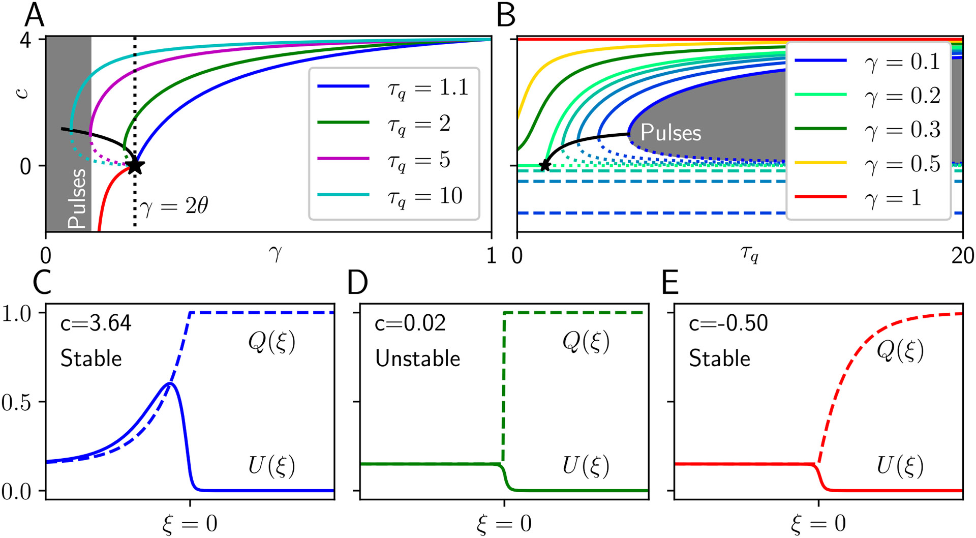
Traveling fronts in a neural field with synaptic depression. A Speeds of stable (solid) and unstable (dashed) traveling fronts as a function of the $\gamma =\frac{1}{1+\beta }$ (synaptic depletion/replenishment timescale ratio). For $\gamma <\theta$, self-consistency is broken, and traveling pulses emerge (see Section 3.2), and for $\theta <\gamma <2\theta$, retreating front solutions emerge (red), with speed and profile independent of ${\tau }_q$. Stable speed $c$ curves coalesce as $\gamma \to 1$ as effects of synaptic depression vanish. B Speeds as a function of synaptic timescale ${\tau }_q$, clearly showing that the speed of retreating fronts is independent of ${\tau }_q$. Black line indicates saddle node bifurcation where the stable and unstable advancing front speeds meet. C, D, E Example profiles of fast stable advancing (blue), slow unstable advancing (green), and retreating (red) fronts. Note the $\xi$-dependent region of $Q(\xi )$ trades places between advancing and retreating cases. For all panels $\theta =0.1$; for the profile panels $\gamma =0.15$ and ${\tau }_q=20$

Fig. 2.

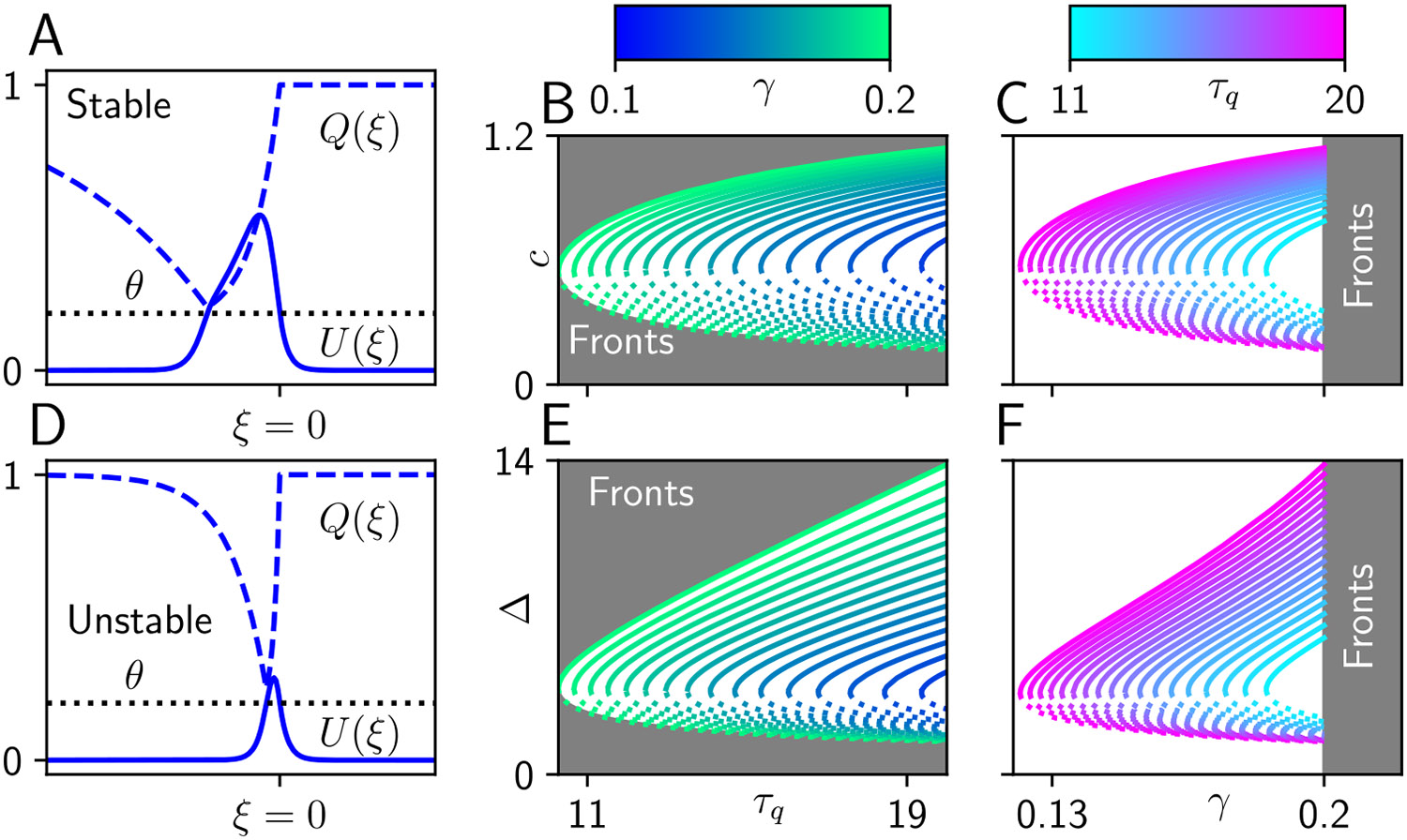
Traveling pulses in a neural field with synaptic depression. A, D Stable and unstable pulse profiles for parameters ${\tau }_q=20$, $\gamma =\frac{1}{6}$, (or equivalently $\beta =5$), and $\theta =0.2$. B, E The pulse speed $c$ and width $\Delta$ are plotted as a function of the synaptic timescale ${\tau }_q$ with color indicating $\gamma$, solid lines indicating stable branches and dotted lines indicating unstable branches. C, F The pulse speed $c$ and width $\Delta$ as a function of $\gamma$ with color indicating ${\tau }_q$, solid lines indicating stable branches and dotted lines indicating unstable branches. We see that as the synaptic efficacy time-scale becomes shorter (${\tau }_q$ small), depression is more rapid and both the width and speed of the pulse shrink. Similarly increasing the strength of depression ($\beta$ large) or equivalently shortening the effective timescale of synaptic depression ($\gamma$ small) will also reduce the width and speed

3.1. Fronts

Changing variables to wave coordinates $\xi =x-ct$ in Eq. (1) and assuming $u\equiv U(\xi )$ and $q\equiv Q(\xi )$, we find that such solutions must satisfy

$$\begin{gathered} -c{U}^{\prime }(\xi )=-U(\xi )+{\int }_{\mathbb{R}}w(\xi -y)Q(y)f(U(y))dy, \\ -c{\tau }_q{Q}^{\prime }(\xi )=1-Q(\xi )-\beta Q(\xi )f(U(\xi )). \end{gathered}$$

Traveling fronts in an excitatory neural field (with $w(x)>0$) with a step nonlinearity $f(u)=H(u-\theta )$ can be shifted such that the single threshold crossing point occurs at $\xi =0$, so that $U(0)=\theta$. The active region is thus $\{\xi \in \mathbb{R}\mid U(\xi )>\theta \}=(-\infty ,0)$. Note, that the function $U(\xi )$ is not necessarily monotone decreasing in $\xi$ as it is in the scalar system due to the negative feedback resulting from synaptic depression. Thus, we must impose an additional inequality $U(\xi )>\theta$ for $\xi <0$, which should be checked for self-consistency:

$$-c{U}^{\prime }(\xi )=-U(\xi )+{\int }_{-\infty }^{0}w(\xi -y)Q(y)dy,$$ (3a)

$$-c{\tau }_q{Q}^{\prime }(\xi )=1-Q(\xi )-\beta Q(\xi )H(-\xi ).$$ (3b)

Equation (3b) is now piecewise linear, decoupled from Eq. (3a), and can be solved piecewise along with enforcing continuity and appropriate boundary conditions depending on the direction $(\text{sign}(c))$ of travel. Before analyzing the case of moving fronts $(c\ne 0)$, we examine the degenerate case of a standing wave solution with speed $c=0$. In this case, Eq. (3b) reduces to a stationary equation, we have $\xi \equiv x$, and the profile of synaptic efficacy is given by

$$Q(x)=\{\begin{array}{cc}1,\hfill & x>0,\hfill \\ \frac{1}{1+\beta }\equiv \gamma ,\hfill & x<0.\hfill \end{array}\phantom{\}}$$

Substituting into Eq. (3a), we see

$$U(x)=\gamma {\int }_{-\infty }^{0}w(x-y)dy,$$

so for a normalized $({\int }_{\mathbb{R}}w(x)dx=1)$ and even $(w(-x)=w(x))$ weight function, we have $\theta =U(0)=\frac{\gamma }{2}$, implying standing fronts only arise for a specific choice of the depression rate $\beta =\frac{1}{2\theta }-1$ which perfectly balances the tendency of the active region to invade inactive regions with the rate of activity decay (Ermentrout and McLeod, 1993).

For forward moving fronts $(c>0)$, we solve Eq. (3b) with the boundary conditions ${\text{lim}}_{\xi \to \infty }Q(\xi )=1$ and ${\text{lim}}_{\xi \to -\infty }Q(\xi )=\gamma$, yielding

$$Q(\xi )=\{\begin{array}{cc}1,\hfill & \xi >0,\hfill \\ \gamma +(1-\gamma )\text{exp}\left(\frac{\xi }{c\gamma {\tau }_q}\right),\hfill & \xi <0.\hfill \end{array}\phantom{\}}$$

Substituting this into Eq. (3a) and solving the $\xi >0$ case with integrating factors gives

$$U(\xi )=e^{\xi ∕c}\left(U_0-\frac{\gamma +c\gamma {\tau }_q}{2(1+c)(1+c\gamma {\tau }_q)}\right)+e^{-\xi }\frac{\gamma +c\gamma {\tau }_q}{2(1+c)(1+c\gamma {\tau }_q)},$$

which we bound as $\xi \to \infty$ by requiring the coefficient on $e^{\xi ∕c}$ to be zero. Recalling that $U(0)=\theta$ we then have

$$\begin{gathered} \theta =\frac{\gamma +c\gamma {\tau }_q}{2(1+c)(1+c\gamma {\tau }_q)} \\ 0=(2\theta \gamma {\tau }_q)c^2+(2\theta +2\theta \gamma {\tau }_q-\gamma {\tau }_q)c+(2\theta -\gamma ), \end{gathered}$$ (4)

whose solutions $c$ are roots of a quadratic:

$$c_{\pm }=\frac{\gamma {\tau }_q-2\theta (1+\gamma {\tau }_q)\pm \sqrt{4{\theta }^2{(1-\gamma {\tau }_q)}^2-4\theta \gamma {\tau }_q(1+\gamma ({\tau }_q-2))+{\gamma }^2{\tau }_q^2}}{4\theta \gamma {\tau }_q},$$

plotted in Fig. 1A, B. This formula makes it clear that a bifurcation occurs when the discriminant is zero, represented by the curve in Fig. 1A. As ${\tau }_q$ increases, this occurs at increasingly smaller values of $\gamma$, eventually below the other front-killing bifurcation arising due to the violation of the self-consistency condition $\gamma \ge \theta$ which we discuss below.

We can also solve the $\xi <0$ case, which automatically satisfies our boundedness condition, and completes the profile for advancing fronts

$$\begin{gathered} U(\xi )=\{\begin{array}{cc}\theta e^{-\xi },\hfill & \xi >0,\hfill \\ \gamma +K_1{e}^{\xi ∕(c\gamma {\tau }_q)}+K_2{e}^{\xi }+(\theta -\gamma -K_1-K_2)e^{\xi ∕c},\hfill & \xi <0,\hfill \end{array}\phantom{\}} \\ {K}_1=\frac{c\gamma {\tau }_q}{1-\gamma {\tau }_q}\cdot \frac{(1-\gamma )c{\gamma }^2{\tau }_q^2}{1-{(c\gamma {\tau }_q)}^2},K_2=-\frac{1}{2(1-c)}\cdot \left(\frac{(1-\gamma )c\gamma {\tau }_q}{1-c\gamma {\tau }_q}-\gamma \right). \end{gathered}$$

The self-consistency inequality ensuring the active region remains superthreshold then requires $\underset{\xi \to -\infty }{\text{lim}}U(\xi )=\gamma >\theta$ or $1∕(1+\beta )>\theta$ implying $\beta <(1-\theta )∕\theta$. Decreasing $\gamma$ below $\theta$ truncates the wave speed branches due to a global bifurcation resulting from the inability of the active region to self-sustain. Profiles are plotted in Fig. 1C, D.

On the other hand, if we assume $c<0$ (retreating fronts), we can similarly find solutions for which the quiescent region invades the active region. We again solve Eq. (3b), with the same boundary conditions, but now having $c<0$ implies

$$Q(\xi )=\{\begin{array}{cc}1+(\gamma -1)e^{\xi ∕(c{\tau }_q)},\hfill & \xi >0,\hfill \\ \gamma ,\hfill & \xi <0.\hfill \end{array}\phantom{\}}$$

Again we substitute into Eq. (3a), enforce boundedness and the threshold condition $U(0)=\theta$. After integrating, we find a condition determining the speed of the front

$$c=\frac{\gamma -2\theta }{2\gamma -2\theta },$$

and a formula for the activity variable of form

$$U(\xi )=\{\begin{array}{cc}\theta e^{-\xi },\hfill & \xi >0,\hfill \\ \gamma +(\theta -\gamma )e^{\xi },\hfill & \xi <0.\hfill \end{array}\phantom{\}}$$ (5)

Speeds are plotted in Fig. 1A, B and example profile in Fig. 1E. Such fronts exist for sufficiently strong depression as bounded by the standing front condition $\beta >(1-2\theta )∕(2\theta )$ or $\gamma <2\theta$, but not too strong ($\beta <(1-\theta )∕\theta$ or $\gamma >\theta$). The speed formula above, corresponding to the red curve in Fig. 1A, shows that as $\gamma \to {\theta }^{+}$ the front speed $c\to -\infty$, resulting in an infinitely rapidly retreating front corresponding to a quiescent state $U\equiv 0$. Retreating fronts can thus be annihilated by excessively strong synaptic depression. On the other hand, as $\gamma \to 2{\theta }^{-}$, the speed $c$ of retreat of the front decreases to zero, leading the stable branch of regressive fronts to join the unstable branch of advancing fronts in a saddle-node bifurcation.

The analysis presented in Fig. 1 builds on that of Kilpatrick and Bressloff (2010b) by examining the covariation of frontspeeds and bifurcations with the strength and timescale of adaptation, especially identifying the important role of regressive fronts in the bifurcation picture. Since spike rate adaptation is not included the model presented here, we have opted to more granularly demonstrate the variation of solution curves as they depend on $\gamma$ and ${\tau }_q$. The use of the derived parameter $\gamma =\frac{1}{1+\beta }$, corresponding to the steady state of synaptic depression, rather than the strength $\beta$, allows us to more clearly shows the global bifurcation from fronts to pulses at $\gamma =\theta$. We also now show the bistable region occurring for portions or all of the interval $\theta <\gamma <2\theta$, due to the emergence of regressive fronts. The branch of regressive fronts (with speed $c<0$) emerges at $\gamma =2\theta$ in a saddle-node bifurcation with the branch of slow unstable advancing fronts (with speed $c>0$). At a lower value of $\gamma$, the branch of these slow advancing fronts annihilates a branch of fast advancing fronts. For $2\theta <\gamma$ only a stable fast front is possible.

The speeds of stable progressing traveling waves decrease with the amplitude $\beta$ of synaptic depression (increasing with $\gamma =1∕(1+\beta )$, the ratio of synaptic depletion and replenishment timescales, Fig.1A). Explicit results on linear stability could be obtained by extending the weak methods developed for piecewise smooth pseudolinear operators developed in Kilpatrick and Bressloff (2010d), but we found reliably that numerical simulations verified stability (instability) of fast (slow) traveling waves across a wide range of parameters. Complementarily, wavespeeds increase with the synaptic depression timescale ${\tau }_q$ (Fig. 1B). Retreating fronts (Fig. 1E) are not simply reflections of advancing fronts (Fig. 1C, D). Rather, an advancing (retreating) front evolves as the active (inactive) region invades the inactive (active) region, so the synaptic depression is constant in the inactive (active) region. These solutions were verified numerically to be stable. In contrast, traveling pulses are always advancing, so that a finite length active region moves into an inactive region, but can be reflected to produce a solution that moves in the opposite direction.

3.2. Pulses

Sufficiently strong synaptic depression produces traveling pulses as negative feedback brings the average voltage $u$ below threshold $\theta$ to create a pulse back (if $\theta >\gamma =\frac{1}{1+\beta }$). These solutions are characterized by both a speed $c$ and width $\Delta$ which are determined by the model parameters.

Changing variables to traveling wave coordinates and considering step nonlinearity $f(u)=H(u-\theta )$, we define an active region $\{\xi \in \mathbb{R}\mid U(\xi )>\theta \}=(-\Delta ,0)$ so the pulse crosses threshold twice at $\theta =U(0)=U(-\Delta )$. In the absence of stimulus, the system Eq. (1) then becomes

$$-c{U}^{\prime }(\xi )=-U(\xi )+{\int }_{-\Delta }^{0}w(\xi -y)Q(y)dy,$$ (6a)

$$-c{\tau }_q{Q}^{\prime }(\xi )=1-Q(\xi )-\beta Q(\xi )[H(\xi +\Delta )-H(\xi )].$$ (6b)

Without loss of generality, we take $c>0$, since backward moving pulses are simply reflections of forward moving pulses. The synaptic efficacy equation is now a decoupled piecewise linear equation. Enforcing the boundary conditions $\underset{\xi \to \pm \infty }{\text{lim}}Q(\xi )=1$, we obtain the solution

$$Q(\xi )=\{\begin{array}{cc}1,\hfill & 0\le \xi ,\hfill \\ \gamma +(1-\gamma )e^{\xi ∕(c\gamma {\tau }_q)},\hfill & -\Delta \le \xi <0,\hfill \\ 1-[1-Q(-\Delta )]e^{(\xi +\Delta )∕(c{\tau }_q)},\hfill & \xi <-\Delta .\hfill \end{array}\phantom{\}}$$

Substituting back into Eq. (6b), we find

$$-c{U}^{\prime }(\xi )=-U(\xi )+\frac{1}{1+\beta }{\int }_{-\Delta }^0(1+\beta e^{(1+\beta )y∕(c{\tau }_q)})w(\xi -y)dy,$$

which can be solved piecewise up to free constants that can be identified by enforcing continuity, boundedness, and boundary conditions. Notice in the limit $\Delta \to \infty$, we recover the equation for $U(\xi )$ in the front case. For the exponential weight function, and the threshold conditions $U(-\Delta )=U(0)=\theta$ we can then obtain the following equations for the wavespeed $c$ and pulsewidth:

$$\theta =\frac{c\gamma {\tau }_q}{2(c+1)(c\gamma {\tau }_q+1)}\left[1-\gamma e^{-\Delta }\left[1+e^{-\Delta ∕(c\gamma {\tau }_q)}\right]\right],$$ (7a)

$$\begin{gathered} \theta =\frac{(2c+1)\gamma }{2(c+1)}(1-e^{-\Delta ∕c})+\frac{\gamma }{2(c-1)}\left[1+\frac{c(1-\gamma ){\tau }_q}{c\gamma {\tau }_q-1}\right](e^{-\Delta }-e^{-\Delta ∕c}) \\ -\frac{c(1-\gamma ){\tau }_q{e}^{-\Delta ∕(c\gamma {\tau }_q)}}{2(c+1)(c\gamma {\tau }_q+1)}+\frac{c^2{\gamma }^3(1-\gamma ){\tau }_q^3(e^{-\Delta ∕(c\gamma {\tau }_q)}-e^{-\Delta ∕c})}{(c^2{\gamma }^2{\tau }_q^2-1)(\gamma {\tau }_q-1)}. \end{gathered}$$ (7b)

Numerical root-finding techniques can subsequently be used to identify the speed $c$ and width $\Delta$ of traveling pulse solutions given implicitly by Eq. (7). For sufficiently weak synaptic depression (corresponding to small $\beta$ and large $\gamma$), there are coexisting branches of (stable) wide and (unstable) narrow traveling pulse solutions (Fig. 2). Increasing either $\gamma$ or ${\tau }_q$ increases the speed and width of the stable traveling pulses. Again, here we have determined wave branch stability by full numerical simulation. With the traveling pulse solutions in hand, and noting they are generally sufficiently wide so interactions between the front and back are weak $(0<e^{-\Delta }\ll 1)$, we now proceed with performing an asymptotic analysis determining how weak forcing modeling sensory input guides the position of a pulse over time.

4. Wave response function

Prior studies of the impact of external inputs on spatiotemporal patterns in neural fields have both considered cases in which direct construction is possible as well as perturbative studies in which the impact of forcing is taken to be weak. Special cases which allow for the calculation of explicit solutions, have revealed the onset of complex dynamics using linear stability or even weakly nonlinear analysis yielding descriptions of breathers (Folias & Bressloff, 2004, 2005; Folias, 2011) or even oscillations reminiscent of perceptual rivalry (Loxley & Robinson, 2009; Kilpatrick & Bressloff, 2010a; Bressloff & Webber, 2012). Numerical studies have also been used to identify the emergence of topological defects in patterns based on transient and localized inputs (Hutt et al., 2003). However, in cases of weak forcing, it is possible to follow the asymptotic approach of Amari (1977), assuming waves or bumps approximately retain their shape but are shifted in space due to the projection of the input along the pattern’s marginally stable direction (Zhang, 1996; Ben-Yishai et al., 1997; Wu et al., 2008b; Burak & Fiete, 2009; Ermentrout et al., 2010; Itskov et al., 2011). Effects of a weak but otherwise arbitrary spatiotemporal input can be approximated by deriving a pattern’s corresponding spatiotemporal filter determined by the adjoint of the linearization about the pattern (Ermentrout et al., 2010; Kilpatrick & Ermentrout, 2012). Such an approach bears resemblance to theory describing how perturbations phase shift nonlinear oscillators, which defines a phase response function (Ermentrout, 1996; Brown et al., 2004), so we refer to our formulation as the wave response function. We consider the impact of a nonlinear auxiliary variable in the neural field (synaptic depression) on such input-response relationships, defining an entrainment problem for a set of periodic spatiotemporal inputs, as a means of framing visual motion processing. Ultimately, this allows us to describe potential neural mechanisms to account for behaviorally reported visual phenomena like the apparent motion illusion.

4.1. General framework

As shown above, in the absence of inputs $(I_u(x,t)\equiv I_q(x,t)\equiv 0)$, Eq. (1) can support traveling wave solutions $(U(\xi ),Q(\xi ))$ that can be determined explicitly for step nonlinearities $f(u)=H(u-\theta )$ and weight kernels with defined integrals. The speed $c$ (and for pulses, the width $\Delta$) can be specified implicitly and thus calculated with root finding. Weak stimulation perturbatively shapes both the profile and position (within the original traveling coordinate frame) of these waves. However, importantly, waves are linearly stable to shape-changing perturbations but marginally stable to those that shift their position within the wave coordinate frame (Amari, 1977; Pinto & Ermentrout, 2001; Coombes & Owen, 2004). Since we treat wave positions as an internal model of the represention of visual object location, we are concerned with wave position shifts as they determine entrainment to moving stimuli of different speeds. To derive an approximate equation for the time-dependent evolution of the wave position $\epsilon \zeta (t)$ relative to the coordinate frame $\xi =x-ct$, we begin by changing variables in Eq. (1) from $(x,t)$ to $(\xi ,t)$. As a result, we have an evolution equation for $u(\xi ,t)$ and $q(\xi ,t)$ defined

$$-c{u}_{\xi }+u_t=-u+w\ast (qf[u])+\epsilon I_u(\xi ,t),$$ (8a)

$$-c{\tau }_q{q}_{\xi }+{\tau }_q{q}_t=1-q-\beta qf[u]+\epsilon I_q(\xi ,t),$$ (8b)

where Eq. (8) generalizes solutions in the traveling frame to allow them to be time-dependent. Effects of external perturbations representing sensory stimuli are then accounted by considering the perturbation expansion

$$u(\xi ,t)=U(\xi -\epsilon \zeta (t))+\epsilon \varphi (\xi -\epsilon \zeta (t),t)+\cdots ,$$ (9a)

$$q(\xi ,t)=Q(\xi -\epsilon \zeta (t))+\epsilon \psi (\xi -\epsilon \zeta (t),t)+\cdots ,$$ (9b)

where $(U(\xi ),Q(\xi ))$ is an unperturbed wave solution and $\epsilon \zeta (t)$ is a small time-dependent function determining position shifts in the traveling coordinates generated by the inputs. The terms $\varphi (\xi )$ and $\psi (\xi )$ weakly modify the wave shape. Plugging the expansion Eq. (9) into Eq. (8), we find the $𝒪(\epsilon )$ terms satisfy the inhomogeneous linear system

$$\left(\begin{array}{c}\hfill {\varphi }_t\hfill \\ \hfill {\tau }_q{\psi }_t\hfill \end{array}\right)+ℒ\left(\begin{array}{c}\hfill \varphi \hfill \\ \hfill \psi \hfill \end{array}\right)={\zeta }^{\prime }(t)\left(\begin{array}{c}\hfill U^{\prime }(\xi )\hfill \\ \hfill {\tau }_q{Q}^{\prime }(\xi )\hfill \end{array}\right)+\left(\begin{array}{c}\hfill I_u(\xi +\epsilon \zeta ,t)\hfill \\ \hfill I_q(\xi +\epsilon \zeta ,t)\hfill \end{array}\right),$$ (10)

where $ℒ$ is the linear operator

$$ℒ\left(\begin{array}{c}\hfill \varphi \hfill \\ \hfill \psi \hfill \end{array}\right)=-c\left(\begin{array}{c}\hfill {\varphi }_{\xi }\hfill \\ \hfill {\tau }_q{\psi }_{\xi }\hfill \end{array}\right)+\left(\begin{array}{c}\hfill \varphi \hfill \\ \hfill \psi \hfill \end{array}\right)+\left(\begin{array}{c}\hfill -w\ast [Q{f}^{\prime }(U)\varphi +\psi f(U)]\hfill \\ \hfill \beta Q{f}^{\prime }(U)\varphi +\beta f(U)\psi \hfill \end{array}\right).$$

A bounded solution of Eq. (10) exists if its right hand side is orthogonal to all elements of the null space of the adjoint operator ${ℒ}^{\ast }$ (Keener 2000a, b; Bressloff 2001). Defining the $L^2$ inner product $\langle \mathbf{f},\mathbf{v}\rangle ={\int }_{\mathbb{R}}{\mathbf{g}}^T(\xi )\mathbf{f}(\xi )d\xi$, we can then identify the adjoint operator by requiring $\langle ℒ\mathbf{u},\mathbf{v}\rangle =\langle \mathbf{u},{ℒ}^{\ast }\mathbf{v}\rangle$. Integrating by parts and rearranging integrals in this equation, we obtain the definition

$${ℒ}^{\ast }\left(\begin{array}{c}\hfill \varphi \hfill \\ \hfill \psi \hfill \end{array}\right)=c\left(\begin{array}{c}\hfill {\varphi }_{\xi }\hfill \\ \hfill {\tau }_q{\psi }_{\xi }\hfill \end{array}\right)+\left(\begin{array}{c}\hfill \varphi \hfill \\ \hfill \psi \hfill \end{array}\right)+\left(\begin{array}{c}\hfill -Q{f}^{\prime }(U)\cdot w\ast \varphi +\beta Q{f}^{\prime }(U)\psi \hfill \\ \hfill -f(U)\cdot w\ast \varphi +\beta f(U)\psi \hfill \end{array}\right),$$ (11)

so the one-dimensional null space ${(v,p)}^T$ defined ${ℒ}^{\ast }{(v,p)}^T={(0,0)}^T$ satisfies the system

$$c{v}_{\xi }=-v+f^{\prime }(U)Q\cdot w\ast v-\beta Q{f}^{\prime }(U)p,$$ (12a)

$$c{\tau }_q{p}_{\xi }=-p+f(U)\cdot w\ast v-\beta f(U)p.$$ (12b)

Note that the terms $f^{\prime }(U)$ will generate delta distributions in the case where $f(U)=H(U-\theta )$. As we will show, the calculation of this derivative must be done with care, but the ensuing system of differential equations can still be solved explicitly by performing integration piecewise and respecting the resulting jump condition. To derive a nonlinear differential equation for the evolution of the wave shift $\zeta (t)$, we apply the boundedness condition for Eq. (10), requiring that ${(v,p)}^T$ is orthogonal to the right hand side of the equation, which can be rearranged to yield

$$\frac{d\zeta }{dt}=-\frac{{\int }_{\mathbb{R}}\left[v(\xi )I_u(\xi +\epsilon \zeta ,t)+p(\xi )I_q(\xi +\epsilon \zeta ,t)\right]d\xi }{{\int }_{\mathbb{R}}{U}^{\prime }(\xi )v(\xi )+{\tau }_q{Q}^{\prime }(\xi )p(\xi )d\xi },$$ (13)

revealing that the leading order description of wave perturbation arises through how the null vector filters inputs to the traveling wave.

Our asymptotic approximation is thus determined implicitly as a solution to the nonlinear and non-autonomous differential equation, Eq. (13). In the rest of this section, we analyze the predictions of this approximation and compare them to numerical simulations in response to transient inputs. In the first case, we will study the impact of an abrupt and spatially homogeneous input upon the relative location of a propagating traveling front, showing the effects of synaptic depression. Second, we examine the effects of spatially localized inputs. Transient and abrupt inputs are assumed to shift in the relative position of the wave $\epsilon \zeta (t)$ at a single localized moment in time, which has the effect of making the terms $I_u(\xi +\epsilon \zeta ,t)$, $I_u(\xi +\epsilon \zeta ,t)$ independent of $\zeta$. Solving Eq. (13) is then trivial as $\zeta (t)$ does not appear in the right hand side. In Section 5 where we consider localized moving stimuli nu does not disappear from the right hand side of Eq. (13) and finding solutions is thus non-trivial.

4.2. Front wave response to a global flash

Here we consider the leading edge position of a traveling front as encoding a position, which is then perturbed by a spatially homogeneous and instantaneous in time input (Fig. 3A). This basic case allows for explicit calculations which will guide our subsequent analysis of moving input tracking. We assume Eq. (13) supports a traveling front solution and is stimulated only through the neural activity variable, $(I_u(\xi ,t),I_q(\xi ,t))=(\delta (t-t_0),0)$, arising via feed-forward input from upstream sensory areas. This could model a weak but broad visual light flash covering the receptive fields of a visual cortical region of interest. Recall that the perturbative scaling $\epsilon$ does not appear in Eq. (13) as these are all factors themselves multiplied by $\epsilon$.

Fig. 3.

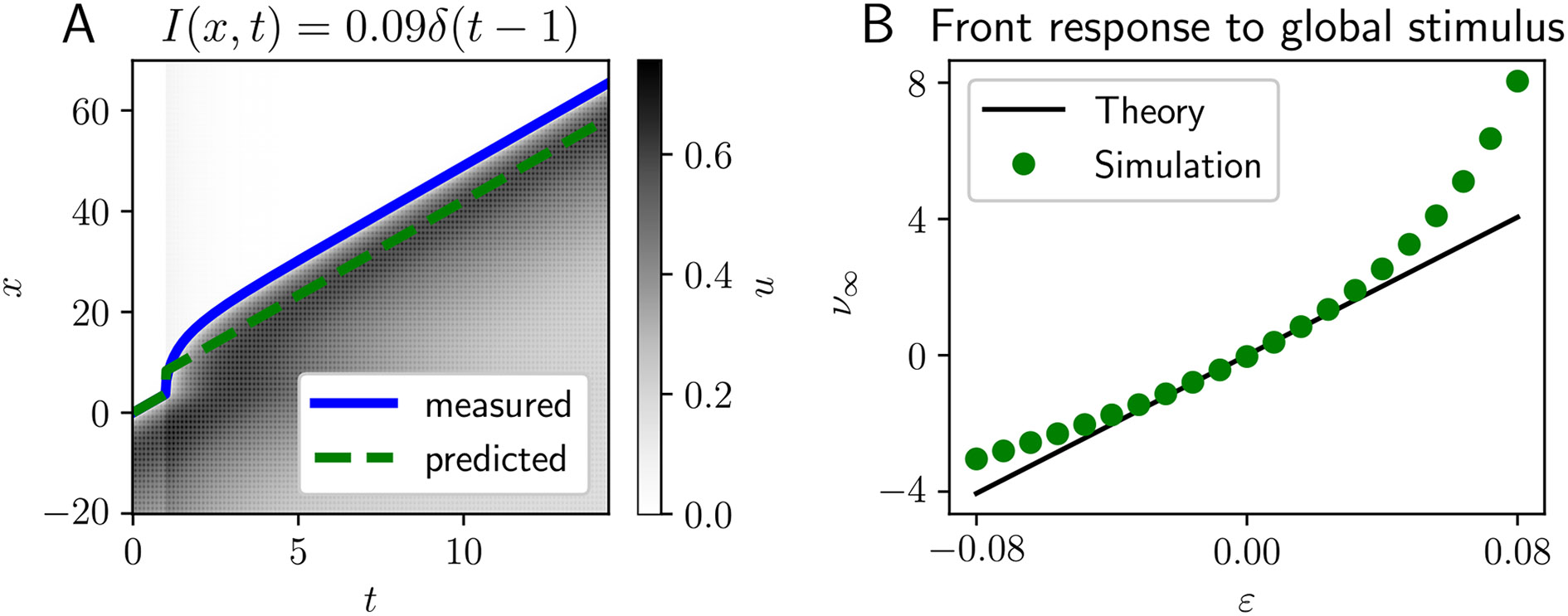
Traveling front advanced by global flash stimulus. A Spatiotemporal evolution of a traveling front perturbed by a spatially homogeneous, temporally pulsatile stimulus $\epsilon I_u(x,t)=\epsilon \delta (t-t_0)$ with $\epsilon =0.09$. We compare the prediction (green dashed line) of our linear theory Eq. (15) to the leading edge computed directly from simulation (blue line). B Wave response function ${\nu }_{\infty }$ predicted by the theory Eq. (15) (black line) and compared to simulations (green dots). Weight function is exponential, firing rate nonlinearity is Heaviside, and model parameters are $\theta =0.1$, $\gamma =0.2$, and ${\tau }_q=20$

We first explicitly calculate the nullspace profile ${(v(\xi ),p(\xi ))}^T$ in the case of a traveling front solution whose adjoint linearization is Eq. (12) with a Heaviside nonlinearity and so satisfying

$$\begin{gathered} c\frac{dv}{d\xi }+v(\xi )=\delta (\xi )\frac{Q(0)}{\mid U^{\prime }(0)\mid }{\int }_{\mathbb{R}}w(y)v(y)dy-\beta \delta (\xi )\frac{Q(0)}{\mid U^{\prime }(0)\mid }p(0), \\ c{\tau }_q\frac{dp}{d\xi }+p(\xi )=H(-\xi ){\int }_{\mathbb{R}}w(\xi -y)v(y)dy-\beta H(-\xi )p(\xi ). \end{gathered}$$

The Heaviside and delta distributions arise from the nonlinearity $f(U(\xi ))=H(U(\xi )-\theta )=H(-\xi )$ and its linearization $f^{\prime }(U(\xi ))=H^{\prime }(U(\xi )-\theta )=\delta (\xi )∕\mid U^{\prime }(0)\mid$ which can be determined by noting

$$-\delta (\xi )=\frac{d}{d\xi }H(-\xi )=\frac{d}{d\xi }H(U(\xi )-\theta )=H^{\prime }(U(\xi )-\theta )U^{\prime }(\xi ).$$

Note the form of the $v(\xi )$ equation, $c{v}^{\prime }(\xi )+v(\xi )=A\delta (\xi )$, suggests a bounded solution of the form $v(\xi )=H(\xi )e^{-\xi ∕c}$, whose step magnitude we are free to pick to be unity. No matter what scaling we pick for this term, it will be canceled in the fraction of Eq. (13) since the terms of the null vector each appear once in the numerator and denominator. Turning then to the $p(\xi )$ equation, we see that for $\xi >0$, it takes the form $\frac{dp}{d\xi }=-\frac{1}{c{\tau }_q}p$ and $p(\xi )=B{e}^{-\xi ∕(c{\tau }_q)}$. On the other half of the domain, $\xi <0$, we substitute the form of $v(\xi )$ and compute the integral for an exponential weight function, finding

$$\frac{dp}{d\xi }+\frac{1}{c\gamma {\tau }_q}p=\frac{1}{2(c+1){\tau }_q}{e}^{\xi },$$ (14)

which can also be solved with a boundedness requirement as $\xi \to -\infty$ to yield a particular solution of form $p(\xi )=C{e}^{\xi }$ whose coefficient can be determined by plugging into Eq.(14). Piecing together the solutions on each half-line using a continuity condition, we find

$$p(\xi )=\frac{c\gamma }{2(c+1)(c\gamma {\tau }_q+1)}\left[e^{\xi }+\left(e^{-\xi ∕(c{\tau }_q)}-e^{\xi }\right)H(\xi )\right].$$

Finally, we recall $(I_u(\xi ,t),I_q(\xi ,t))=(\delta (t-t_0),0)$ in Eq. (13) for this particular scenario and integrate with respect to time to find

$$\zeta (t)=\frac{2(c+1){(c\gamma {\tau }_q+1)}^2}{2\theta {(c\gamma {\tau }_q+1)}^2-(1-\gamma )\gamma {\tau }_q}H(t-t_0).$$ (15)

We demonstrate this prediction and compare to numerical simulations in Fig. 3B. Note, we generally underestimate the degree to which the front is advanced because this is a global stimulus and so higher order nonlinear effects further speed along the front while it remains away from equilibrium. However for sufficiently small $\epsilon$, the linear approximation is reasonably close. Using a second-order centered finite difference approximation, we find that $\frac{d}{d\epsilon }{{\zeta }_{\infty }(\epsilon )\mid }_{\epsilon =0}$ agrees with the scaling Eq. (15) with a relative error of 0.17% (attributed to errors in the simulation and finite difference approximation).

This analysis would be easy to repeat for a retreating front. Based on our observations here, we expect that global stimuli would cause the front to push outward, so positive stimuli delay rather than advance the position of the front relative to the wave coordinate frame.

Taking the limit of no synaptic depression $\gamma \to 1^{-}$, we see we recover

$$\underset{\gamma \to 1^{-}}{\text{lim}}\zeta (t)=\frac{c+1}{\theta }H(t-t_0)=\frac{H(t-t_0)}{2{\theta }^2},$$

which was derived previously in Kilpatrick and Ermentrout (2012). Note well that because we are not considering persistent stimuli here, the dependence upon $\nu$ on the right-hand-side of Eq. (13) does not come into effect and so it is straightforward to solve the equation by integration. As noted, spatially global stimuli perturb waves in ways that are not always well captured by linear theory, but more spatially localized stimuli have a more modest effect on wave position, which can also be captured well by our linear theory as we now show.

4.3. Pulse wave response

Traveling front solutions are unaffected by activity $(I_u)$ perturbations behind their leading edge $(\xi <0)$ as demonstrated above. On the other hand, traveling pulses have both a front and back which can be perturbed by weak inputs. Moreover, spatially localized inputs that may model the position of a visual object interact with wave position in ways that depend on their width as well as strength. To better understand the dynamics of such interactions as a means of building a theory of visual object tracking, we begin by deriving the nullspace of the adjoint operator in the case of a traveling pulse. Taking a Heaviside nonlinearity in Eq. (12) we find

$$\begin{gathered} c\frac{dv}{d\xi }+v=\delta (\xi )\frac{Q(0)}{\mid U^{\prime }(0)\mid }\cdot \left[{\int }_{\mathbb{R}}w(y)v(y)dy-\beta p(0)\right] \\ +\delta (\xi +\Delta )\frac{Q(-\Delta )}{\mid U^{\prime }(-\Delta )\mid }\cdot \left[{\int }_{\mathbb{R}}w(y+\Delta )v(y)dy-\beta p(-\Delta )\right], \end{gathered}$$ (16a)

$$c{\tau }_q\frac{dp}{d\xi }+p=[H(\xi +\Delta )-H(\xi )]\cdot \left[{\int }_{\mathbb{R}}w(\xi -y)v(y)dy-\beta p(\xi )\right],$$ (16b)

where again the right-hand-side of Eq. (16a) is singularized due to the derivative of the step nonlinearities $f(U(\xi )-\theta )=H(\xi +\Delta )-H(\xi )$ such that

$$\begin{gathered} \delta (\xi +\Delta )-\delta (\xi )=\frac{d}{d\xi }[H(\xi +\Delta )-H(\xi )] \\ =\frac{d}{d\xi }H(U(\xi )-\theta )=H^{\prime }(U(\xi )-\theta )U^{\prime }(\xi ). \end{gathered}$$

Eq. (16a) has the form $c{v}^{\prime }(\xi )+v(\xi )=A\delta (\xi )+B\delta (\xi +\Delta )$ suggesting the following ansatz $v(\xi )=\frac{1}{c}[A_{0}H(\xi )e^{-\xi ∕c}+A_{-\Delta }H(\xi +\Delta )e^{-(\xi +\Delta )∕c}$ whose coefficients satisfy the linear system

$$c{A}_0=\frac{Q(0)}{\mid U^{\prime }(0)\mid }\cdot \left[A_{0}G(0)+A_{-\Delta }G(-\Delta )-\beta cp(0)\right],$$ (17a)

$$c{A}_{-\Delta }=\frac{Q(-\Delta )}{\mid U^{\prime }(-\Delta )\mid }\cdot \left[A_{0}G(\Delta )+A_{-\Delta }G(0)-\beta cp(-\Delta )\right],$$ (17b)

where we have defined the integral function

$$G(z)={\int }_z^{\infty }w(y)e^{-(y-z)∕c}dy.$$

To solve this linear system, we need to determine $p(\xi )$ to constrain its values at $\xi =0,-\Delta$. Of course, recall ${(v,p)}^T$ is a vector eigensolution and so can be freely scaled. As such, we should expect the two equations in Eq. (17) are linearly dependent, so we need only solve one.

We thus next examine Eq. (16b) in pieces. First, along $\xi <-\Delta$, we find a simple homogeneous equation $c{\tau }_q{p}^{\prime }(\xi )=-p(\xi )$ whose solution must be bounded as $\xi \to -\infty$, so $p(\xi )=0$ on this portion of the domain implying $p(-\Delta )=0$. Then on $-\Delta <\xi <0$, we can rewrite the equation as

$$\frac{dp}{d\xi }+\frac{1}{c\gamma {\tau }_q}p(\xi )=\frac{1}{c^2{\tau }_q}\left[A_{0}G(-\xi )+A_{-\Delta }G(-\Delta -\xi )\right],$$ (18)

which we can integrate with the boundary condition $p(-\Delta )=0$ to find

$$p(\xi )=\frac{e^{-\xi ∕(c\gamma {\tau }_q)}}{c^2{\tau }_q}\cdot \left[A_{0}J(\xi ,0)+A_{-\Delta }J(\xi ,-\Delta )\right],$$ (19)

where we have defined

$$J(\xi ,z)={\int }_{-\Delta }^{\xi }G(z-y)e^{y∕(c\gamma {\tau }_q)}dy.$$

Evaluating Eq. (19) at $\xi =0$ to find the remaining term in the self-consistency Eq. (17),

$$p(0)=\frac{A_0}{c^2{\tau }_q}J(0,0)+\frac{A_{-\Delta }}{c^2{\tau }_q}J(0,-\Delta ).$$

Substituting into the consistency conditions Eq. (17), we have that $A_0$ and $A_{-\Delta }$ satisfy the singular linear system

$$\begin{gathered} \left[\frac{\mid U^{\prime }(0)\mid }{Q(0)}c+\frac{\beta }{c{\tau }_q}J(0,0)-G(0)\right]A_0+\left[\frac{\beta }{c{\tau }_q}J(0,-\Delta )-G(-\Delta )\right]A_{-\Delta }=0 \\ -G(\Delta )A_0+\left[\frac{\mid U^{\prime }(-\Delta )\mid }{Q(-\Delta )}c-G(0)\right]\cdot A_{-\Delta }=0. \end{gathered}$$

Ignoring the trivial solution $A_0=A_{-\Delta }=0$ and fixing the first entry $A_0=1$, we may solve this singular equation by satisfying the second equation to find

$$A_{-\Delta }=\frac{G(\Delta )\cdot Q(-\Delta )}{c\mid U^{\prime }(-\Delta )\mid -G(0)\cdot Q(-\Delta )},$$ (20)

so by defining $A_{-\Delta }$ as in Eq. (20) and $A_0=1$, we find the one-dimensional nullspace of ${ℒ}^{\ast }$ is spanned by ${(v(\xi ),p(\xi ))}^T$ where

$$v(\xi )=H(\xi )e^{-\xi ∕c}+A_{-\Delta }H(\xi +\Delta )e^{-(\xi +\Delta )∕c},$$ (21a)

$$p(\xi )=\frac{e^{-\xi ∕(c\gamma {\tau }_q)}}{c^2{\tau }_q}\cdot \left[J(\xi ,0)+A_{-\Delta }J(\xi ,-\Delta )\right].$$ (21b)

To study the impact of spatially locaized and temporally pulsatile stimuli on traveling pulses, we again use Eq. (13) to formulate an approximation to the phase advance of the pulse from an abrupt input at a single point in time,

$$\zeta (t)=-\epsilon \frac{{\int }_{x_0-\Delta x∕2}^{x_0+\Delta x∕2}\left[{\overline{I}}_u\cdot v(\xi )+{\overline{I}}_q\cdot p(\xi )\right]d\xi }{{\int }_{\mathbb{R}}{U}^{\prime }(\xi )v(\xi )+{\tau }_q{Q}^{\prime }(\xi )p(\xi )d\xi }H(t-t_0).$$ (22)

Integrating against both perturbations of the neural activity of amplitude ${\overline{I}}_u$ and synaptic efficacy of amplitude ${\overline{I}}_q$ variables, we adjust the position $x_0$ of the stimulus relative to the pulse and see the approximation agrees well with numerical simulations (Fig. 4). Note that the effect of inputs is stronger (See axis scaling on Fig. 4A vs B) when applied to the neural activity variable (${\overline{I}}_u>0$ and ${\overline{I}}_q\equiv 0$). Taking the width of the stimulus to zero $\Delta x\to 0^{+}$ and its amplitude arbitrarily strong (${\overline{I}}_u\to \infty$ or ${\overline{I}}_q\to \infty$), the input approaches a delta distribution in space and the integral in Eq. (22) is proportional to the nullspace as a function of $x_0$. Generally, we find contributions to the phase advance of the wave are quite weak when originating at the back (threshold crossing) of the pulse $(A_{-\Delta }\approx 0)$ as can be seen by evaluating Eq. (20) across a wide range of parameters. Thus, pulses are only substantially perturbed by inputs at their front.

Fig. 4.

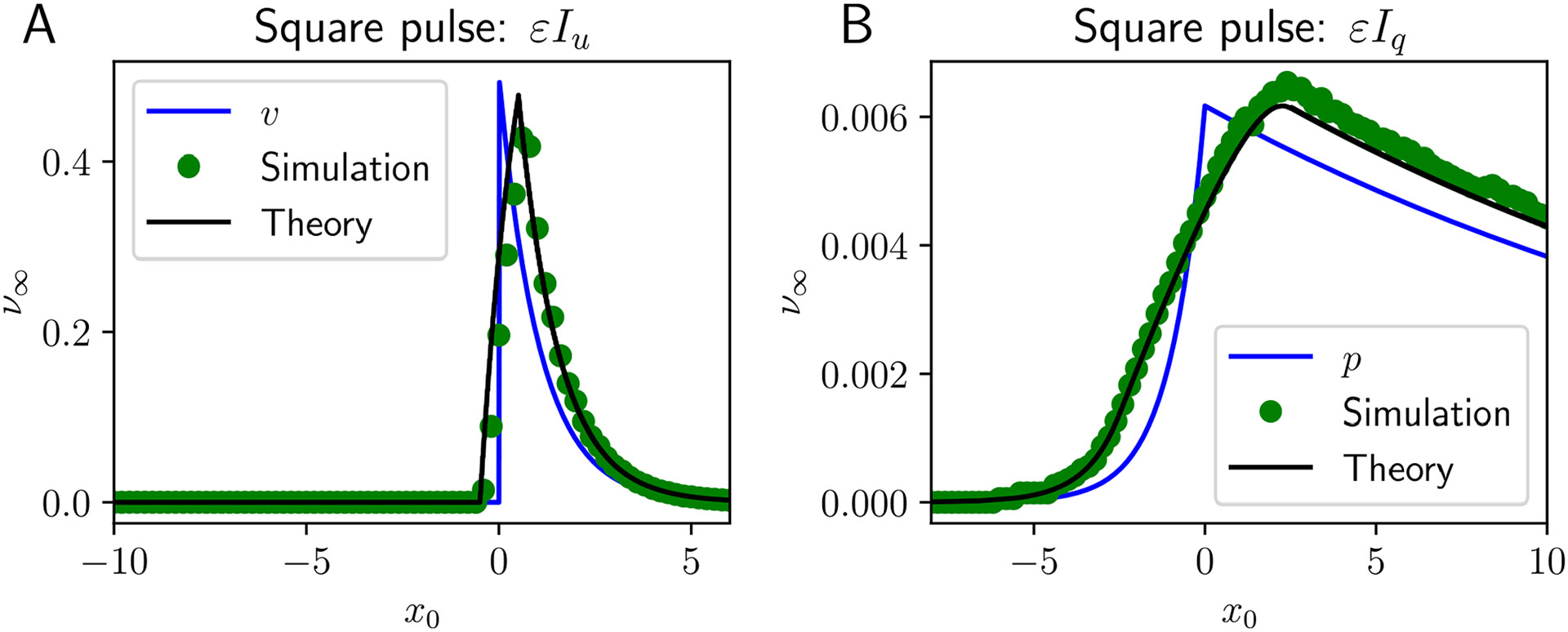
Response of traveling pulse to localized pulsatile square stimulus. Stimuli $\epsilon I_j(x,t)=\epsilon {\overline{I}}_j\delta (t)P(x,x_0,{\Delta }_x)(j=u,q)$ are centered in space $P(x,x_0,{\Delta }_x)=H(x-x_0+\Delta x∕2)-H(x-x_0-{\Delta }_x∕2)$ at $x_0$ with width ${\Delta }_x=1$ and presented at time $t=0$ either to A the neural activity variable: ${\overline{I}}_u=1$ and $I_q\equiv 0$; or B the synaptic efficacy variable: ${\overline{I}}_q=1$ and ${\overline{I}}_u=0$. Asymptotic theory (black line) approximates the results from numerical simulation (green dots) very well. Note that the spatially square pulse input shifts and widens the core null space function (blue curve), which describes how the wave filters forcing. Other parameters are $\theta =0.2$, $\gamma =1∕6$, ${\tau }_q=20$, and $\epsilon =0.05$

Our experiments for simple stimuli (spatially homogeneous inputs to fronts, Fig. 3; and square wave pulses to traveling pulses, Fig. 4) result in trivial differential equations we can solve by integrating due to the stimulus being localized to a single point in time. When stimuli varying non-trivially in space and time, we must heed the nonlinear nature of the asymptotic approximation of the wave phase given by the differential Eq. (13). In the next section, we demonstrate that the recurrence represented in this nonlinear equation allows us to better approximate the effects of persistent as well as periodic stimuli providing a simplified theory for predicting the entrainment of traveling waves to localized moving stimuli.

5. Entrainment to moving and apparently moving stimuli

We now describe an asymptotic theory of the encoding of moving objects by the position of perturbed traveling waves. In the absence of stimulation, Eq. (1) supports traveling wave solutions that move at a fixed natural wavespeed. A wave’s leading edge is interpreted as the visually encoded position of a moving object. When objects move at speeds other than the natural wavespeed, external stimulation must be able to shift the phase and/or increase the speed of the wave to appropriately encode the position. Sensory input is modeled as a spatially localized but moving stimulus $I_u$ with a different speed. We will say such a stimulus entrains a wave if the wave’s speed is altered so as to match that of the stimulus (Alamia and VanRullen 2023).

Our wave response approximation Eq. (13) can be used to predict conditions for the entrainment of traveling pulses to both persistent and moving stimuli as well as intermittent flashing stimuli meant to mimic the forcing common to the apparent motion illusion. As opposed to the theory developed previously for the tracking of persistent and moving stimuli (Folias & Bressloff, 2005; Wu et al., 2008b), flashing stimuli that hop require a periodic map-based theory to determine conditions on speed and input amplitude for perceived motion. We begin by examining a perturbative theory of tracking persistent and moving stimuli first.

5.1. Front entrainment

For simplicity, and to demonstrate the techniques we will use to determine entrainment, we first consider a moving step stimulus defined

$$\epsilon I_u(x,t)=\epsilon H\left[(c+{\Delta }_c)t-x\right].$$ (23)

applied to a traveling front solution to Eq. (1). For the purposes of this calculation, we consider the propagation of the step at $x=(c+{\Delta }_c)t$ as the location of this stimulus. Note, we will take the difference of the input speed $c+{\Delta }_c$ and natural wavespeed $c$ to be positive ${\Delta }_c>0$ so the wave must catch up to the input. We are concerned with deriving conditions on the strength $\epsilon$ and speed offset ${\Delta }_c$ of the input that allow for the perturbed wave’s speed to match that of the input (entrainment). When the input leads the wave, it will speed the wave up beyond its natural speed, and if the stimulus is sufficiently strong and slow, the perturbed wavespeed will catch up to that of the input, so the front lags the stimulus at a distance that remains bounded in time. Stimuli that are too fast and/or weak, however, will outrun the wave, so the distance between them grows in time (and entrainment fails). Analyzing Eq. (13), we will determine the relation between input parameters and boundaries of entrainment as well as the distance entrained fronts lag inputs.

For inputs that drive only the neural activity variable of traveling fronts, we find the associated component of the nullspace filtering the input is $v(\xi )=H(\xi )e^{-\xi ∕c}$. Note, the wave will only be affected by inputs ahead of the front. Moreover, upon defining the scaling factor

$$K\equiv \langle U^{\prime },v\rangle +{\tau }_q\langle Q^{\prime },p\rangle$$

that appears in the denominator of Eq. (13), we can simplify the expression for ${\zeta }^{\prime }(t)$. Now, upon assuming the input is initially ahead of the front, and recalling $\xi =x-ct$, so $H(ct-x+{\Delta }_{c}t)=H(-\xi +{\Delta }_{c}t)$, we have

$$\begin{gathered} K\frac{d\zeta }{dt}={\int }_{\mathbb{R}}v(\xi )I_u(\xi +\epsilon \zeta )d\xi \\ ={\int }_0^{\infty }H(-(\xi +\epsilon \zeta -{\Delta }_{c}t))e^{-\xi ∕c}d\xi \\ =c\left(1-e^{(\epsilon \zeta -{\Delta }_{c}t)∕c}\right) \end{gathered}$$

Applying the change of variables $y(t)=\epsilon \zeta (t)-{\Delta }_{c}t$, we can define $y(t)<0$ as the time-dependent lag of the front behind the stimulus, and we find

$$\begin{gathered} K\frac{y^{\prime }+{\Delta }_c}{\epsilon }=c\cdot \left(1-e^{y∕c}\right), \\ \frac{dy}{dt}=-{\Delta }_c+\frac{\epsilon c}{K}\cdot \left(1-e^{y∕c}\right) \end{gathered}$$ (24)

Since this is now an autonomous differential equation and assuming the stimulus is ahead of the front $(y<0)$, we can derive a corresponding fixed point $y_{\infty }<0$ under the condition ${\Delta }_c<\frac{\epsilon c}{K}$. The equilibrium is specified by the equation

$${\Delta }_c=\frac{\epsilon c}{K}\left(1-e^{y_{\infty }∕c}\right)\Rightarrow y_{\infty }=c\log \left(1-\frac{{\Delta }_{c}K}{\epsilon c}\right).$$ (25)

When ${\Delta }_c\ge \frac{\epsilon c}{K}$, the solution defined in Eq. (25) does not exist, and the stimulus speed $(c+{\Delta }_c)$ is too fast for the wave to entrain. Eq. (24) can also be solved directly, yielding

$$y(t)=c\log \frac{\epsilon c-{\Delta }_{c}K}{\epsilon c+\left((\epsilon c-{\Delta }_{c}K)e^{-y_0∕c}-\epsilon c\right)\cdot \text{exp}\left[-\frac{\epsilon c-{\Delta }_{c}K}{cK}\cdot t\right]},$$

where $y(0)=y_0$. In the limit as $t\to \infty$, we find $y(t)\to y_{\infty }$ as expected.

5.2. Localized stimulation of fronts and pulses

Our theory describes visual object inputs as localized in space, which can for instance be associated with square waves with some finite width ${\Delta }_x$ and speed displacement ${\Delta }_c$ beyond the natural wavespeed. Specifically, we define our stimulus by

$$\epsilon I_u(\xi ,t)=\epsilon \left[H\left(-(\xi -{\Delta }_{c}t)\right)-H\left(-(\xi +{\Delta }_x-{\Delta }_{c}t)\right)\right].$$ (26)

Taking ${\Delta }_x\to \infty$, we can recover the traveling front stimulus as in the previous section.

Consider the effect the input has upon the front at different displacements. When the front of the stimulus is ahead of the front’s leading edge, but the active region of Eq. (26) still contains the front $({\Delta }_{c}t\in [0,{\Delta }_x])$, only the part of the stimulus ahead of the front will be filtered by the adjoint nullspace, the same as before. Thus, only the portion of the stimulus ahead of or containing the leading edge of the front has any effect on the location of the leading edge of the pulse. Either a fixed point is reached, or the lag becomes larger than the width of the square stimulus and the impact of the stimulus on the front weakens further. We expect the front will then lose the opportunity to entrain to the stimulus at this point, implying entrainment generally must occur before the entire stimulus slips ahead of the leading edge. When solving for the corresponding fixed point of Eq. (24), this generates the stricter entrainment condition

$${\Delta }_c<\epsilon \frac{c}{K}(1-e^{-{\Delta }_x∕c}).$$ (27)

Stability of the fixed point described by Eq. (25) can be determined in the same way as before showing it is stable.

Boundaries on entrainment for traveling pulses are determined similarly, except that the activity nullspace term has the form $v(\xi )=H(\xi )e^{-\xi ∕c}+A_{-\Delta }H(\xi +\Delta )e^{-(\xi +\Delta )∕c}$. However, the slow timescale ${\tau }_q\gg 1$ of the synaptic efficacy results in $\mid A_{-\Delta }\mid \ll 1$ across a wide range of parameters. This again gives us an entrainment threshold described by Eq. (27) and a corresponding lag described by Eq. (25), where the pulse speed $c$ and factor $K$ are now determined by the roots of Eq. (7) and the appropriate inner product, respectively. As expected, in simulations, a stimulus with speed close enough to the natural speed of the pulse will entrain it (Fig. 5A), but if the stimulus speed is too far from the natural speed of the pulse, the pulse slips behind the stimulus indefinitely (Fig. 5B). For weak stimuli, we find that the theory developed here accurately predicts the boundary between entrainment failure and success accurately for corresponding simulations (Fig. 5C).

Fig. 5.

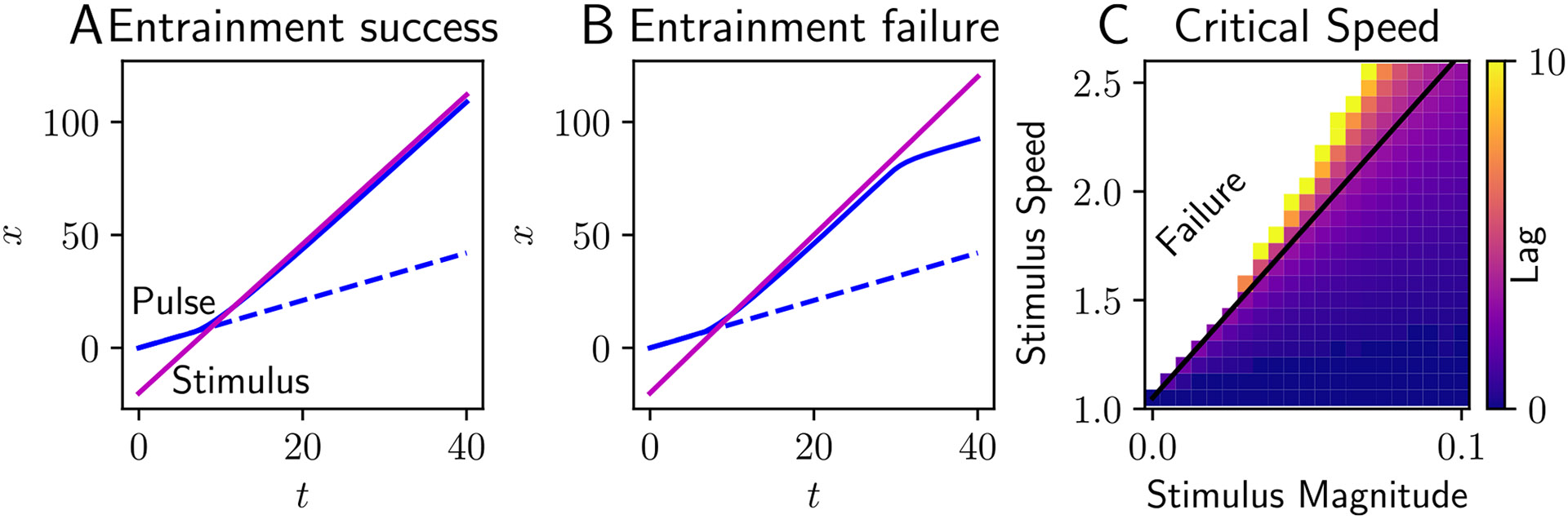
Entrainment of traveling pulses to propagating square pulses. A Spatiotemporal location of the leading edge of a traveling pulse (solid blue) perturbed by a moving square input (magenta) is ahead of that of the unperturbed pulse (dashed blue). Stimulus has magnitude $\epsilon =0.1$ and speed $c+{\Delta }_c=3.3$ (compare to natural wavespeed $c\approx 1.051$). Pulse remains entrained indefinitely. B When stimulus speed $c+{\Delta }_c=3.5$ is too large, the stimulus eventually slips off the pulse, which relaxes to its original speed. C Numerical simulations reveal a (white) region of failed entrainment when the stimulus speed is too large for a given magnitude $\epsilon$. Otherwise the colored region indicates the lag $y_{\infty }$ of entrained pulses whose stimulus speeds are not too large. Our first order approximation of the entrainment boundary (Eq. (27), black line) matches well. Neural field model parameters are $\theta =0.2$, $\gamma =1∕6$, ${\tau }_q=20$ and stimulus width ${\Delta }_x=10$

5.3. Pulse entrainment to apparent motion

Apparent motion is modeled here by flashing stimuli whose positions move between but not during flashes (i.e., on periods of the stimulus). In this case, the driven solution does not converge to a proper traveling wave, but a solution that is periodic under a fixed spatial shift given by the movement of the flashing stimuli. Dividing the time domain into segments of length $T$, the period of the forcing stimulus, we define the length of the on phase of length $T_{\text{on}}<T$, during which there is a square pulse input, and off phase of length $T_{\text{off}}=T-T_{\text{on}}$, during which there is no input. The stimulus is advanced by $(c+{\Delta }_c)T$ between on phases, and we thus call ${\Delta }_c$ the speed offset of the input. Such a stimulus can be expressed using indicator functions by

$$\begin{gathered} \epsilon I_u(x,t)=\epsilon {ℐ}_{(x^{\ast }-{\Delta }_x,x^{\ast })}\left(x-\lfloor \frac{t}{T}\rfloor (c+{\Delta }_c)T\right) \\ \cdot {ℐ}_{(0,T_{\text{on}})}\left(t-\lfloor \frac{t}{T}\rfloor T\right), \end{gathered}$$

where we have defined the indicator function ${ℐ}_A(x)$ of a subdomain $A$ with argument $x$ as

$${ℐ}_A(x)=\{\begin{array}{cc}1,\hfill & \text{if}x\in A,\hfill \\ 0,\hfill & \text{else}.\hfill \end{array}\phantom{\}}$$

Changing variables $(x,t)$ to $(\xi ,t)$ and using our simplifying approximation $A_{-\Delta }\approx 0$ and substituting into Eq. (13) and making the change of variables $y=\epsilon \nu +ct$, we can approximate the movement of the leading edge $y$ of the front when it is inside the stimulus,

$$\frac{dy}{dt}=c+\frac{\epsilon c}{K}\left(1-e^{-{\Delta }_x∕c}{e}^{y∕c}\right),$$

which can be solved assuming $y(0)=y_0$ is the location of the wave front at time $t=0$, to find

$$\begin{gathered} y(t)=-c\log \\ \left[\frac{\epsilon }{K+\epsilon }{e}^{-{\Delta }_x∕c}+\left(e^{-y_0∕c}-\frac{\epsilon }{K+\epsilon }{e}^{-{\Delta }_x∕c}\right)e^{-(K+\epsilon )t∕K}\right]\equiv F(t;y_0), \end{gathered}$$

so the function $F(t;y_0)$ describes how the input maps $y$ forward from $y_0$ after a time $t$. During the off phase, $y$ will simply advance according to the natural wavespeed, so the approximate solution in the first period $T$ is

$$y(t)=\{\begin{array}{cc}F(t,y_0),\hfill & 0\le t\le T_{\text{on}}\hfill \\ F(T_{\text{on}},y_0)+(t-T_{\text{on}})c,\hfill & T_{\text{on}}\le t\le T.\hfill \end{array}\phantom{\}}$$ (28)

Subtracting off $(c+{\Delta }_c)T$, we can determine where the wave front $y$ will be at time $t=T$ relative to the newly flashed stimulus

$$y_1=F(T_{\text{on}},y_0)-c{T}_{\text{on}}-{\Delta }_{c}T.$$

Thus, we can inductively define a map describing how the next relative location of the wave front $y_{n+1}$ depends on the current location $y_n$ as

$$y_{n+1}=F(T_{\text{on}},y_n)-c{T}_{\text{on}}-{\Delta }_{c}T.$$ (29)

We shall consider wave front entrainment to the periodic, moving, and flashing stimulus possible when the map Eq. (29) has a stable fixed point described by the condition

$$y^{\ast }=F(T_{\text{on}},y^{\ast })-c{T}_{\text{on}}-{\Delta }_{c}T,$$

which can be solved to find

$$y^{\ast }={\Delta }_x-c\log \left[\frac{\epsilon }{K+\epsilon }\cdot \frac{e^{T_{\text{on}}}-e^{-\epsilon T_{\text{on}}∕K}}{e^{-{\Delta }_{c}T∕c}-e^{-\epsilon T_{\text{on}}∕K}}\right].$$ (30)

The denominator of the argument in the logarithm above is positive, and the solution is defined if ${\Delta }_c<\epsilon \frac{T_{\text{on}}}{T}\frac{c}{K}$. Linearizing the map Eq. (29) and plugging in the solution Eq. (30), we find its stability is determined by the single eigenvalue $\lambda =\text{exp}\left[\frac{{\Delta }_{c}T}{c}-\frac{\epsilon T_{\text{on}}}{K}\right]$, so $\lambda \in (0,1)$ if ${\Delta }_c<\epsilon \frac{T_{\text{on}}}{T}\frac{c}{K}$, which implies that the fixed point defining periodic entrainment is stable whenever it exists.

Our theory is consistent with the result of numerical simulations of the response of traveling waves to periodic, moving, and flashing stimuli. Flashing stimuli that are sufficiently strong and that travel at a speed that is not too much faster than the natural wavespeed will entrain the traveling wave (Fig. 6A). Tracking the leading edges of these flash-forced traveling pulses reveals that the stimulus speeds up the wave while it is on, and the pulse speed relaxes to its natural value between flashes. Over time, the average speed of the forced solution matches that of the average speed $c+{\Delta }_c$ of the forcing stimulus. On the other hand, if (a) the distance traveled with each hop between flashes is too large or (b) the stimulus is too weak or short, then the pulse will not be sped up enough during the on phase of the period. As a result, the pulse will eventually lag further and further behind the forcing stimulus as time goes on (Fig. 6B). The combined necessity of having a forcing stimulus whose speed difference is not too large $({\Delta }_c)$, whose magnitude is not too weak $(\epsilon )$, or whose on phase is not too short $(T_{\text{on}})$ is all contained in the entrainment boundary inequality ${\Delta }_c<\epsilon \frac{T_{\text{on}}}{T}\frac{c}{K}$. Indeed, we see that this boundary well approximates the boundary we can determine from numerical simulations (Fig. 6C).

Fig. 6.

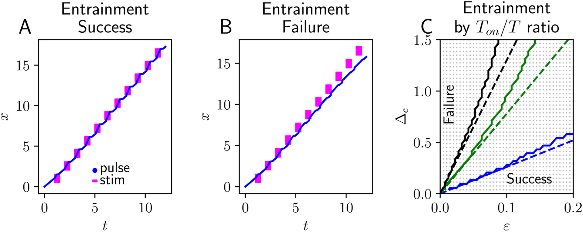
Wave entrainment to apparently moving stimuli. A The leading edge (blue line) of a traveling pulse becomes entrained to an intermittent, moving, and flashing stimulus (magenta indicates regions where stimulus is non-zero). The difference between the baseline wavespeed $(c\approx 1.051)$ and the effective speed of the forcing stimulus is ${\Delta }_c=0.5$; its magnitude is $\epsilon =0.2$; its width and starting position are ${\Delta }_x=1$ and $x^{\ast }=0$; on and off phases are $T_{\text{on}}=T_{\text{off}}=0.5$ for a total stimulus period of $T=1$. B Weakening the stimulus magnitude to $\epsilon =0.12$, the traveling pulse fails to entrain, and slips ever further behind the stimulus. C. Asymptotic approximation to the entrainment boundary (dashed line) ${\Delta }_c=\epsilon \frac{T_{\text{on}}}{T}\frac{c}{K}$ is well matched to results of numerical simulations (solid) separating the domain of entrainment (lower right) from entrainment failure (upper left). Increasing the ratio $T_{\text{on}}∕T_{\text{off}}$ enlarges the domain of entrainment. Blue: $T_{\text{on}}∕T_{\text{off}}=0.1∕0.5=0.2$; Green: $T_{\text{on}}∕T_{\text{off}}=0.5∕0.5=1$; Black: $T_{\text{on}}∕T_{\text{off}}=0.5∕0.1=5$. Stimulus width is ${\Delta }_x=10$; all other model parameters are same. Throughout, neural field model parameters are $\theta =0.2$, $\gamma =1∕6$, and ${\tau }_q=20$

Thus we find that the entrainment of neural activity waves in a model of sensory cortex can be described by a relatively accessible theory. Akin to results from past work on phase response theory, we find that stimuli whose speed is close enough to the natural speed can indeed entrain waves. This applied not only to persistent traveling stimuli but also flashing stimuli, suggesting a neuromechanistic theory for the generation of apparent motion illusions in visual cortex.

5.4. Extensions to planar models

Our analysis so far has focused on one-dimensional networks for simplicity and because effective stimulus speed strongly determines the emerges of apparent motion perception (Gepshtein and Kubovy, 2007). However, curvature and other geometric features of a stimulus’ trajectory could also affect such percepts, so it is reasonable to extend our models to two-dimensional domains, to more completely characterize the possible motion of inputs from the visual field. Neural field models can produce traveling spots in two-dimensions when some form of negative feedback is incorporated into a network with lateral inhibition (Lu et al., 2011; Coombes et al., 2012). Activity bumps that would be marginally stable in the absence of negative feedback destabilize, and can travel in any radial direction depending on initial conditions. The centroid of the traveling spot may then be considered as a position-encoder, as with the leading edge of the front or pulse in one-dimension.

The planar version of Eq. (1) involves convolving the integral over ${\mathbb{R}}^2$, requiring radially symmetric weights $w(x-y)=w(r)$ now where $r=\Vert x-y\Vert$ (Folias and Bressloff, 2004). In particular, we consider the following wizard hat lateral inhibitory weight kernel $w(r)=2e^{-r}(1-r)$, and the sigmoid nonlinearity $f(u)={\left(1+e^{-\eta (u-\theta )}\right)}^{-1}$. Rather than taking the high-gain limit $(\eta \to \infty )$, we consider a smooth nonlinearity $(\eta <\infty )$ allowing for accurate simulation results with coarser grids. Fig. 7 demonstrates two cases of stimulus-perturbed traveling spot, showing how a stimulus that is too weak or at a sharp angle will not entrain the spot. A traveling spot begins (Fig. 7A) propagating rightward until reaching an intersection point with a Gaussian stimulus $\epsilon I_u(x,t)=\epsilon e^{-{\mid x-vt\mid }^2∕2}$ (where now $x$ and $\nu$ are vectors) traveling at an oblique angle (Fig. 7B). Parameters have been tuned so that the bump $\mid c\mid \approx 0.07$ and stimulus $\mid \nu \mid \approx 0.08$ speed. The traveling bump entrains to the stronger ($\epsilon =0.3$, Fig. 7C) but not the weaker ($\epsilon =0.2$, Fig. 7D) stimulus. Moving stimuli thus can entrain traveling bumps in planar domains, depending on the stimulus strength and trajectory.

Fig. 7.

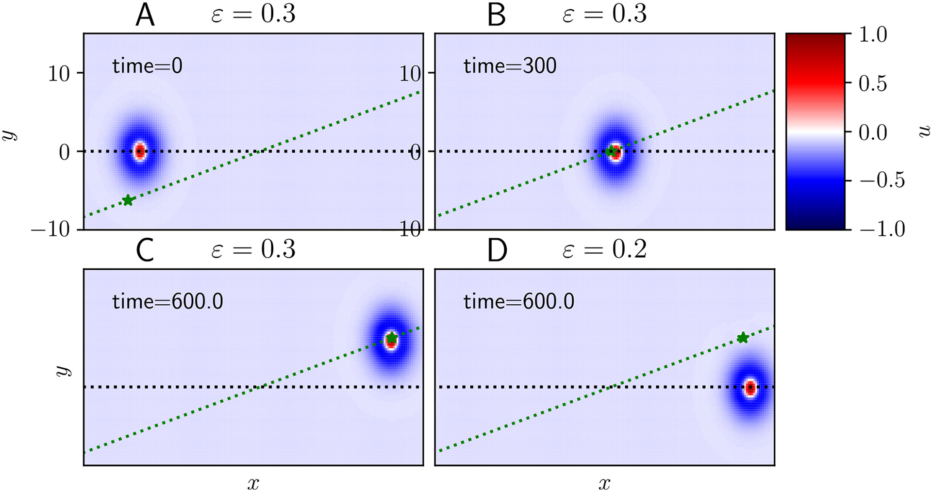
Entrainment success vs. failure in a 2D model. Simulations of Eq. (1) in two-dimensions $(n=2)$ with a lateral inhibitory kernel $w(r)=2e^{-r}(1-r)$, and sigmoidal firing rate function $f(u)={(1+e^{-\eta (u-\theta )})}^{-1}$. A We initialize a spot that propagates rightward (along the black dashed line) and apply an obliquely moving Gaussian stimulus $\epsilon I_u(x,t)=\epsilon e^{-{\Vert x-vt\Vert }^2∕2}$ (star moving along dashed green line). B Stimulus meets spot. C Sufficiently strong $(\epsilon =0.3)$ stimulus entrains spot, changing its course. D Weak stimulus $(\epsilon =0.2)$ fails to entrain. Other parameters are $\eta =20$, $\theta =0.2$, ${\tau }_q=20$, and $\gamma =0.5$

6. Discussion

In this paper, we have developed and analyzed a neuronal network model describing the stimulus-response relationships of traveling activity waves to moving inputs. Our model incorporates negative feedback in the form of short-term synaptic depression, which attenuates activity at the back of the waves, generating traveling pulses when it is strong enough. The nonlinear model of synaptic depression can be derived directly from spiking models (Tsodyks et al., 1998), and is more physiologically motivated than heuristic linear negative feedback models (Pinto and Ermentrout, 2001). In the absence of inputs, we can explicitly derive conditions for the emergence of traveling fronts and pulses, along with their speed and width. Building on past work (Kilpatrick and Bressloff, 2010b), we have identified conditions for the coexistence of stable progressing and receding fronts. Using asymptotic theory, we have derived a general formula describing how traveling fronts and pulses respond to generalized external input. Our formula can consider inputs either to the neural activity or synaptic efficacy variables. This framework was then used to perturbatively quantify the effect of different moving stimuli on the phase of traveling waves. The nonlinear differential equation accounts for how past perturbations have shifted the wave when considering the effect of future inputs.

Weak external stimuli shift the position of traveling waves relative to their natural position, which changes linearly in time as they propagate. Extending prior work (Kilpatrick and Ermentrout, 2012), we have demonstrated how the impact of inputs both on the leading and trailing edge of a traveling pulse impacts the wave phase, though in general the effect of the trailing edge is weak compared to the leading edge due to the exponential dependence on distance. The key predictions we have made using this theory focus on entrainment phenomena, whether a traveling wave will lock to an external moving stimulus traveling at a different speed. The natural speed of the wave in addition to the strength and relative speed of the input, rather than the width of the stimulus, are most important for making these predictions when inputs are persistent. Indeed propagating neural activity patterns in medial temporal (MT) cortex have been shown to encode object motion direction and speed, suggesting these waves play an important role in neural information processing (Townsend et al., 2017). However, given that neural activity waves can propagate spontaneously or can persist after an initial stimulus has been removed (Xu et al., 2007), such persistent activity could represent illusory sensory stimuli in the absence of inputs. Our theory demonstrates that propagating waves can be perturbed to match their speed to intermittent stimuli that jump locations between flashes, providing a simple quantitative measure to determine whether such entrainment is expected based on the strength and temporal properties of the input.

Our reduced equations describe the movement of a traveling wave’s leading edge relative to the location of a stimulus, allowing us to identify both the fixed points and the transient dynamics of the edge in the coordinate frame of the moving input. For persistent and moving inputs, this corresponds to the solution of a nonlinear differential equation, which we can obtain explicitly. For intermittent flashing stimuli, we frame the entrainment problem as a fixed point analysis of a map, describing the updated location of the edge after each temporal period of the stimulus. Intermittent stimuli must be stronger than corresponding persistent stimuli to entrain wave motion, consistent with observations that real motion is encoded more readily than apparent motion (Merchant et al., 2003). Our asymptotic techniques allow us to derive a simple formula for the entrainment boundary, which intuitively quantifies the increasing relative speeds that can be entrained as the on phase of the flash grows longer.

Extensions to planar cases where the input follows more complex trajectories (e.g., reversing the direction of the bump) would be interesting to consider. Adaptive effects of synaptic depression would suppress activity in the wake of the traveling spot, potentially extinguishing traveling spots that cross back over previously visited paths. It would be interesting to study how these predictions align with psychophysical responses from experiments in future studies.

The response of traveling waves to external stimuli has been measured in vivo and in vitro (Wu et al. 2008a), demonstrating inputs speed up (Richardson et al., 2005), displace or annihilate (Gao et al., 2012), or even switch the direction (Pang et al., 2020) of waves. These response properties reflect a highly dynamic and spatiotemporal form of input processing in sensory cortices (Ermentrout & Kleinfeld, 2001; Muller et al., 2018). Disentangling the role of synaptic network architecture in spatiotemporal processing thus requires the analysis of dynamic and mechanistic neural network models that capture cortical complexity while still being amenable to reductions that identify key system input-output relationships. Our analysis has developed a powerful and reduced understanding of how a spatially structured network can encode apparent motion, a phenomenon originally reported in non-invasive behavioral experiments (Anstis, 1980; Ramachandran & Anstis, 1986) and more recently shown to correspond to elevations of activity in visual cortex in corresponding regions of perceived motion (Muckli et al., 2005; Blom et al., 2020). Activation of visual stimulus-encoding neurons in the absence of a stimulus may suggest the anticipation a temporarily occluded and moving object’s reappearance as in the phenomenon of visual preplay (Ekman et al., 2017; Aitken et al., 2020). Our results could guide future behavioral and neurophysiological experiments linking psychophysical thresholds for apparent motion to the coordination of visual cortical activity and external inputs.

Our model builds on prior abstract and Bayesian models accounting for classic psychophysical and quantitative observations of apparent motion. Spatial and temporal intervals between object presentations strongly determine the strength of apparent motion (Korte, 1915; Burt & Sperling, 1981). When individuals report a strong motion percept from successively flashed stimuli for a certain pair of intervals, changing the interval of one feature (space or time) reduces report strength unless the other feature is changes (increased or decreased) similarly (Koffka, 2013; Kolers, 2013). While the details of this relationship continue to be debated (Gepshtein and Kubovy, 2007), and people have a bias towards reporting the slowest consistent motion speed (Ullman, 1979; Wallach, 1935), there is relative consensus that subjects infer speed sequentially (Hürlimann et al., 2002; Stocker & Simoncelli, 2006). Such strategies can be described by inferential models that use Bayesian sequential analysis to predict probabilistic estimates humans make of illusory motion (Weiss et al., 2002). However, these theories neglect a mechanistic understanding of such inference. Recent efforts like (Chemla et al., 2019) have shown such possibilities in a limited context, though the models are not tractable enough to make psychophysical predictions. Our model demonstrates the dynamic process by which an input suggestive of apparent motion drives activity in a neural circuit to relax to a representation consistent with an apparent motion report. The model also quantitatively predicts specific thresholds on the difference $({\Delta }_c)$ between an ideal apparent motion speed ($c$) and the speed of the flashing stimulus. The range of possible speeds increases with the fraction of time the stimulus is flashed $(T_{on}∕T)$ and its brightness $(\epsilon )$. These concrete predictions could be validated and even fit to data extracting psychophysical thresholds from motion lattice experiments as in (Gepshtein and Kubovy, 2007).

Our model could be extended to provide mechanisms for extinguishing traveling waves encoding irrelevant stimulus locations. For sufficiently strong inputs representing flashing stimuli, counterpropagating traveling pulses can be nucleated (Kilpatrick and Bressloff, 2010b), one of which would annihilate the errant lagging pulse. Another interesting possibility would be to consider tuning the model slightly beyond the saddle-node bifurcation of traveling pulses, so that the wave was no longer self-sustaining and would eventually die if far enough from the external input. Dynamics of this ghost of a traveling pulse (Dahlem, 2013) could still be characterized using a normal form analysis (Kilpatrick and Faye, 2014) by perturbing about the saddle-node bifurcation to jointly characterize the postion and amplitude of the wave. In addition, we could extend the model to include mechanisms whereby inputs would slow the wave in addition to speeding it up, allowing persistent or flashing stimuli traveling at speeds less than the intrinsic wave speed to entrain waves. Waves in neural fields with lateral inhibitory weight kernels have wave response functions with both positive and negative parts (Kilpatrick and Ermentrout, 2012), supporting wave synchronization in uncoupled networks receiving common inputs (Kilpatrick, 2015). As with neural oscillators (Abouzeid and Ermentrout, 2009), we expect response functions with parts of both sign are better for synchrony and entrainment across a diversity of inputs. Even in our current network waves can be slowed by presenting negative inputs, so an auxiliary feedback system that would tune effective sensory input polarity to errors in stimulus location prediction could also allow our model to support entrainment to input speeds slower than the natural wave speed.

A number of modeling assumptions could be relaxed, only costing the explicit tractability of the model, but without sacrificing the core mechanisms of the model. Waves, their linearizations, and eigenfunctions can all be calculated using alternative numerical methods such as shooting (Ermentrout et al., 2010) or Fourier methods in approximating partial differential equation models (Coombes et al., 2007) in order to carry out a similar analysis for smooth firing rate functions, more sophisticated weight functions, or compact domains. We also note that the existence of retreating fronts suggests there may be parameter regimes where we could exploit the slow timescale of depression and invoke singular perturbation theory (Pinto and Ermentrout, 2001), constructing a traveling pulse from advancing and retreating fronts of the same speed. Distinct excitatory/inhibitory populations could be considered or additionally short term facilitation to more fully capture the diversity of static and dynamic models of synaptic transmission and understand how these contribute to the filtering properties of traveling waves. Similar analyses could also be applied to planar neural field models, building on past work which has developed perturbative theory based on a spectral analysis of linearized problems to understanding how the closed boundary of a stationary or moving bump responds to external inputs (Coombes et al., 2012).

References

- Abouzeid A, & Ermentrout B (2009). Type-ii phase resetting curve is optimal for stochastic synchrony. Physical Review E, 80(1), 011911. [DOI] [PubMed] [Google Scholar]
- Aitken F, Menelaou G, Warrington O, et al. (2020). Prior expectations evoke stimulus-specific activity in the deep layers of the primary visual cortex. PLoS biology, 18(12), e3001023. [DOI] [PMC free article] [PubMed] [Google Scholar]
- Alamia A, & VanRullen R (2023). A traveling waves perspective on temporal binding. Journal of Cognitive Neuroscience, pp 1–9. [DOI] [PubMed] [Google Scholar]
- Amari S. (1977). Dynamics of pattern formation in lateral-inhibition type neural fields. Biological Cybernetics, 27(2), 77–87. [DOI] [PubMed] [Google Scholar]
- Anstis SM (1980). The perception of apparent movement. Philosophical Transactions of the Royal Society of London B, Biological Sciences, 290(1038), 153–168. [DOI] [PubMed] [Google Scholar]
- Bart E, Bao S, & Holcman D (2005). Modeling the spontaneous activity of the auditory cortex. Journal of Computational Neuroscience, 19(3), 357–378. [DOI] [PubMed] [Google Scholar]
- Ben-Yishai R, Hansel D, & Sompolinsky H (1997). Traveling waves and the processing of weakly tuned inputs in a cortical network module. Journal of computational neuroscience, 4, 57–77. [DOI] [PubMed] [Google Scholar]
- Bill J, Gershman SJ, & Drugowitsch J (2022). Visual motion perception as online hierarchical inference. Nature Communications, 13(1), 7403. [DOI] [PMC free article] [PubMed] [Google Scholar]
- Blom T, Feuerriegel D, Johnson P, et al. (2020). Predictions drive neural representations of visual events ahead of incoming sensory information. Proceedings of the National Academy of Sciences, 117(13), 7510–7515. [DOI] [PMC free article] [PubMed] [Google Scholar]
- Born RT, & Bradley DC (2005). Structure and function of visual area mt. Annu Rev Neurosci, 28, 157–189. [DOI] [PubMed] [Google Scholar]
- Bressloff PC (2001). Traveling fronts and wave propagation failure in an inhomogeneous neural network. Physica D: Nonlinear Phenomena, 155(1), 83–100. [Google Scholar]
- Bressloff PC (2011). Spatiotemporal dynamics of continuum neural fields. Journal of Physics A: Mathematical and Theoretical, 45(3), 033001. [Google Scholar]
- Bressloff PC, & Webber MA (2012). Neural field model of binocular rivalry waves. Journal of Computational Neuroscience, 32(2), 233. [DOI] [PubMed] [Google Scholar]
- Bressloff PC, Folias SE, Prat A, et al. (2003). Oscillatory waves in inhomogeneous neural media. Physical review letters, 91(17), 178101. [DOI] [PubMed] [Google Scholar]
- Brown E, Moehlis J, & Holmes P (2004). On the phase reduction and response dynamics of neural oscillator populations. Neural computation, 16(4), 673–715. [DOI] [PubMed] [Google Scholar]
- Burak Y, & Fiete IR (2009). Accurate path integration in continuous attractor network models of grid cells. PLoS computational biology, 5(2), e1000291. [DOI] [PMC free article] [PubMed] [Google Scholar]
- Burt P, & Sperling G (1981). Time, distance, and feature trade-offs in visual apparent motion. Psychological review, 88(2), 171. [PubMed] [Google Scholar]
- Chemla S, Reynaud A, Di Volo M, et al. (2019). Suppressive traveling waves shape representations of illusory motion in primary visual cortex of awake primate. Journal of Neuroscience, 39(22), 4282–4298. [DOI] [PMC free article] [PubMed] [Google Scholar]
- Cichy RM, Pantazis D, & Oliva A (2014). Resolving human object recognition in space and time. Nature neuroscience, 17(3), 455–462. [DOI] [PMC free article] [PubMed] [Google Scholar]
- Coombes S. (2005). Waves, bumps, and patterns in neural field theories. Biol Cybern, 93, 91–108. [DOI] [PubMed] [Google Scholar]
- Coombes S, & Owen MR (2004). Evans functions for integral neural field equations with heaviside firing rate function. SIAM Journal on Applied Dynamical Systems, 3(4), 574–600. [Google Scholar]
- Coombes S, Venkov NA, Shiau L, et al. (2007). Modeling electrocortical activity through improved local approximations of integral neural field equations. Physical Review E, 76(5), 051901. [DOI] [PubMed] [Google Scholar]
- Coombes S, Schmidt H, & Bojak I (2012). Interface dynamics in planar neural field models. The Journal of Mathematical Neuroscience, 2(1), 1–27. [DOI] [PMC free article] [PubMed] [Google Scholar]
- Dahlem MA (2013). Migraine generator network and spreading depression dynamics as neuromodulation targets in episodic migraine. Chaos: An Interdisciplinary Journal of Nonlinear Science, 23(4), 046101. [DOI] [PubMed] [Google Scholar]
- Eckert MP, & Zeil J (2001). Towards an ecology of motion vision. Motion vision: computational, neural, and ecological constraints, pp 333–369. [Google Scholar]
- Ekman M, Kok P, & de Lange FP (2017). Time-compressed preplay of anticipated events in human primary visual cortex. Nature Communications, 8(1), 15276. [DOI] [PMC free article] [PubMed] [Google Scholar]
- Erlhagen W, & Schöner G (2002). Dynamic field theory of movement preparation. Psychological review, 109(3), 545. [DOI] [PubMed] [Google Scholar]
- Ermentrout B. (1996). Type i membranes, phase resetting curves, and synchrony. Neural computation, 8(5), 979–1001. [DOI] [PubMed] [Google Scholar]
- Ermentrout B. (1998). Neural networks as spatio-temporal pattern-forming systems. Reports on progress in physics, 61(4), 353. [Google Scholar]
- Ermentrout GB, & Kleinfeld D (2001). Traveling electrical waves in cortex: Insights from phase dynamics and speculation on a computational role. Neuron, 29(1), 33–44. [DOI] [PubMed] [Google Scholar]
- Ermentrout GB, & McLeod JB (1993). Existence and uniqueness of travelling waves for a neural network. Proceedings of the Royal Society of Edinburgh: Section A Mathematics, 123(3), 461–478. [Google Scholar]
- Ermentrout GB, Jalics JZ, & Rubin JE (2010). Stimulus-driven traveling solutions in continuum neuronal models with a general smooth firing rate function. SIAM Journal on Applied Mathematics, 70(8), 3039–3064. [Google Scholar]
- Faye G, & Kilpatrick ZP (2018). Threshold of front propagation in neural fields: An interface dynamics approach. SIAM Journal on Applied Mathematics, 78(5), 2575–2596. [Google Scholar]
- Folias SE (2011). Nonlinear analysis of breathing pulses in a synaptically coupled neural network. SIAM Journal on Applied Dynamical Systems, 10(2), 744–787. [Google Scholar]
- Folias SE, & Bressloff PC (2004). Breathing pulses in an excitatory neural network. SIAM Journal on Applied Dynamical Systems, 3(3), 378–407. [Google Scholar]
- Folias SE, & Bressloff PC (2005). Stimulus-locked traveling waves and breathers in an excitatory neural network. SIAM journal on Applied Mathematics, 65(6), 2067–2092. [Google Scholar]
- Fortune ES, & Rose GJ (2001). Short-term synaptic plasticity as a temporal filter. Trends in neurosciences, 24(7), 381–385. [DOI] [PubMed] [Google Scholar]
- Gepshtein S, & Kubovy M (2007). The lawful perception of apparent motion. Journal of Vision, 7(8), 9–9. [DOI] [PubMed] [Google Scholar]
- Goulet J, & Ermentrout GB (2011). The mechanisms for compression and reflection of cortical waves. Biological cybernetics, 105, 253–268. [DOI] [PubMed] [Google Scholar]
- Han F, Caporale N, & Dan Y (2008). Reverberation of recent visual experience in spontaneous cortical waves. Neuron, 60(2), 321–327. [DOI] [PMC free article] [PubMed] [Google Scholar]
- Huang X, Troy WC, Yang Q, et al. (2004). Spiral waves in disinhibited mammalian neocortex. Journal of Neuroscience, 24(44), 9897–9902. [DOI] [PMC free article] [PubMed] [Google Scholar]
- Hürlimann F, Kiper DC, & Carandini M (2002). Testing the bayesian model of perceived speed. Vision research, 42(19), 2253–2257. [DOI] [PubMed] [Google Scholar]
- Hutt A, Bestehorn M, & Wennekers T (2003). Pattern formation in intracortical neuronal fields. Network: Computation in Neural Systems, 14(2), 351. [PubMed] [Google Scholar]
- Itskov V, Hansel D, & Tsodyks M (2011). Short-term facilitation may stabilize parametric working memory trace. Frontiers in computational neuroscience, 5, 40. [DOI] [PMC free article] [PubMed] [Google Scholar]
- Kane SA, & Zamani M (2014). Falcons pursue prey using visual motion cues: new perspectives from animal-borne cameras. Journal of Experimental Biology, 217(2), 225–234. [DOI] [PMC free article] [PubMed] [Google Scholar]
- Keener JP (2000a). Homogenization and propagation in the bistable equation. Physica D: Nonlinear Phenomena, 136(1), 1–17. [Google Scholar]
- Keener JP (2000b). Propagation of waves in an excitable medium with discrete release sites. SIAM Journal on Applied Mathematics, 61(1), 317–334. [Google Scholar]
- Kilpatrick ZP (2015). Stochastic synchronization of neural activity waves. Physical Review E, 91(4), 040701. [DOI] [PubMed] [Google Scholar]
- Kilpatrick ZP (2018). Synaptic mechanisms of interference in working memory. Scientific Reports, 8(1), 1–20. [DOI] [PMC free article] [PubMed] [Google Scholar]
- Kilpatrick ZP, & Bressloff PC (2010a). Binocular rivalry in a competitive neural network with synaptic depression. SIAM Journal on Applied Dynamical Systems, 9(4), 1303–1347. [Google Scholar]
- Kilpatrick ZP, & Bressloff PC (2010b). Effects of synaptic depression and adaptation on spatiotemporal dynamics of an excitatory neuronal network. Physica D: Nonlinear Phenomena, 239(9), 547–560. [Google Scholar]
- Kilpatrick ZP, & Bressloff PC (2010c). Spatially structured oscillations in a two-dimensional excitatory neuronal network with synaptic depression. Journal of Computational Neuroscience, 28(2), 193–209. [DOI] [PubMed] [Google Scholar]
- Kilpatrick ZP, & Bressloff PC (2010d). Stability of bumps in piecewise smooth neural fields with nonlinear adaptation. Physica D: Nonlinear Phenomena, 239(12), 1048–1060. [Google Scholar]
- Kilpatrick ZP, & Ermentrout B (2012). Response of traveling waves to transient inputs in neural fields. Physical Review E, 85, 021910. [DOI] [PubMed] [Google Scholar]
- Kilpatrick ZP, & Faye G (2014). Pulse bifurcations in stochastic neural fields. SIAM Journal on Applied Dynamical Systems, 13(2), 830–860. [Google Scholar]
- Kilpatrick ZP, Folias SE, & Bressloff PC (2008). Traveling pulses and wave propagation failure in inhomogeneous neural media. SIAM Journal on Applied Dynamical Systems, 7(1), 161–185. [Google Scholar]
- Knill DC, & Pouget A (2004). The bayesian brain: the role of uncertainty in neural coding and computation. TRENDS in Neurosciences, 27(12), 712–719. [DOI] [PubMed] [Google Scholar]
- Koffka K. (2013). Principles of Gestalt psychology, (Vol. 44). Routledge. [Google Scholar]
- Kolers PA (2013). Aspects of motion perception: International series of monographs in experimental psychology, (Vol. 16). Elsevier. [Google Scholar]
- Korte A. (1915). Kinematoskopische untersuchungen. Zeitschrift fur Psychologie, 65. [Google Scholar]
- Loxley P, & Robinson P (2009). Soliton model of competitive neural dynamics during binocular rivalry. Physical review letters, 102(25), 258701. [DOI] [PubMed] [Google Scholar]
- Lu Y, Sato Y, & Amari Si. (2011). Traveling bumps and their collisions in a two-dimensional neural field. Neural Computation, 23(5), 1248–1260. [DOI] [PubMed] [Google Scholar]
- Merchant H, Battaglia-Mayer A, & Georgopoulos AP (2003). Interception of real and apparent motion targets: psychophysics in humans and monkeys. Experimental Brain Research, 152, 106–112. [DOI] [PubMed] [Google Scholar]
- Muckli L, Kohler A, Kriegeskorte N, et al. (2005). Primary visual cortex activity along the apparent-motion trace reflects illusory perception. PLoS biology, 3(8), e265. [DOI] [PMC free article] [PubMed] [Google Scholar]
- Muller L, Chavane F, Reynolds J, et al. (2018). Cortical travelling waves: mechanisms and computational principles. Nature Reviews Neuroscience, 19(5), 255–268. [DOI] [PMC free article] [PubMed] [Google Scholar]
- Nagy M, Ákos Z, Biro D, et al. (2010). Hierarchical group dynamics in pigeon flocks. Nature, 464(7290), 890–893. [DOI] [PubMed] [Google Scholar]
- O’Reilly JX, Mesulam MM, & Nobre AC (2008). The cerebellum predicts the timing of perceptual events. Journal of Neuroscience, 28(9), 2252–2260. [DOI] [PMC free article] [PubMed] [Google Scholar]
- Pang Z, Alamia A, & VanRullen R (2020). Turning the stimulus on and off changes the direction of a traveling waves. Eneuro, 7(6). [DOI] [PMC free article] [PubMed] [Google Scholar]
- Pinto DJ, & Ermentrout GB (2001), Spatially structured activity in synaptically coupled neuronal networks: I. traveling fronts and pulses. SIAM Journal on Applied Mathematics, 62(1), 206–225. [Google Scholar]
- Ramachandran VS, & Anstis SM (1986). The perception of apparent motion. Scientific American, 254(6), 102–109. [DOI] [PubMed] [Google Scholar]
- Richardson KA, Schiff SJ, & Gluckman BJ (2005). Control of traveling waves in the mammalian cortex. Physical review letters, 94(2), 028103. [DOI] [PMC free article] [PubMed] [Google Scholar]
- Stocker AA, & Simoncelli EP (2006). Noise characteristics and prior expectations in human visual speed perception. Nature neuroscience, 9(4), 578–585. [DOI] [PubMed] [Google Scholar]
- Tenenbaum JB, Kemp C, Griffiths TL, et al. (2011). How to grow a mind: Statistics, structure, and abstraction. Science, 331(6022), 1279–1285. [DOI] [PubMed] [Google Scholar]
- Torney CJ, Hopcraft JGC, Morrison TA, et al. (2018). From single steps to mass migration: the problem of scale in the movement ecology of the serengeti wildebeest. Philosophical Transactions of the Royal Society B: Biological Sciences, 373(1746), 20170012. [DOI] [PMC free article] [PubMed] [Google Scholar]
- Townsend RG, Solomon SS, Martin PR, et al. (2017). Visual motion discrimination by propagating patterns in primate cerebral cortex. Journal of Neuroscience, 37(42), 10074–10084. [DOI] [PMC free article] [PubMed] [Google Scholar]
- Tsodyks M, Pawelzik K, & Markram H (1998). Neural networks with dynamic synapses. Neural Computation, 10(4), 821–835. [DOI] [PubMed] [Google Scholar]
- Ullman S. (1979). The interpretation of visual motion. Massachusetts Inst of Technology Pr. [Google Scholar]
- Venkov NA, Coombes S, & Matthews PC (2007). Dynamic instabilities in scalar neural field equations with space-dependent delays. Physica D: Nonlinear Phenomena, 232(1), 1–15. [Google Scholar]
- Wallach H. (1935). Über visuell wahrgenommene bewegungsrichtung. Psychologische Forschung, 20, 325–380. [Google Scholar]
- Weiss Y, Simoncelli EP, & Adelson EH (2002). Motion illusions as optimal percepts. Nature neuroscience, 5(6), 598–604. [DOI] [PubMed] [Google Scholar]
- Wilson HR, & Cowan JD (1973). A mathematical theory of the functional dynamics of cortical and thalamic nervous tissue. Kybernetik, 13(2), 55–80. [DOI] [PubMed] [Google Scholar]
- Gao X, Xu W, Wang Z, Takagaki K, Li B, Wu JY (2012). Interactions between two propagating waves in rat visual cortex. Neuroscience, 216, 57–69. [DOI] [PMC free article] [PubMed] [Google Scholar]
- Wu JY, Huang X, & Zhang C (2008a). Propagating waves of activity in the neocortex: What they are, what they do. The Neuroscientist, 14(5), 487–502. [DOI] [PMC free article] [PubMed] [Google Scholar]
- Wu S, Hamaguchi K, & Amari Si. (2008b). Dynamics and computation of continuous attractors. Neural computation, 20(4), 994–1025. [DOI] [PubMed] [Google Scholar]
- Xie X, Hahnloser RH, & Seung HS (2002). Double-ring network model of the head-direction system. Physical Review E, 66(4), 041902. [DOI] [PubMed] [Google Scholar]
- Xu W, Huang X, Takagaki K, et al. (2007). Compression and reflection of visually evoked cortical waves. Neuron, 55(1), 119–129. [DOI] [PMC free article] [PubMed] [Google Scholar]
- York LC, & van Rossum MC (2009). Recurrent networks with short term synaptic depression. Journal of computational neuroscience, 27(3), 607. [DOI] [PubMed] [Google Scholar]
- Zanos TP, Mineault PJ, Nasiotis KT, et al. (2015). A sensorimotor role for traveling waves in primate visual cortex. Neuron, 85(3), 615–627. [DOI] [PubMed] [Google Scholar]
- Zhang K. (1996). Representation of spatial orientation by the intrinsic dynamics of the head-direction cell ensemble: a theory. Journal of Neuroscience, 16(6), 2112–2126. [DOI] [PMC free article] [PubMed] [Google Scholar]