



Abstract
The manner in which neural activity unfolds over time is thought to be central to sensory, motor and cognitive functions in the brain. Network models have long posited that the brain’s computations involve time courses of activity that are shaped by the underlying network. A prediction from this view is that the activity time courses should be difficult to violate. We leveraged a brain–computer interface to challenge monkeys to violate the naturally occurring time courses of neural population activity that we observed in the motor cortex. This included challenging animals to traverse the natural time course of neural activity in a time-reversed manner. Animals were unable to violate the natural time courses of neural activity when directly challenged to do so. These results provide empirical support for the view that activity time courses observed in the brain indeed reflect the underlying network-level computational mechanisms that they are believed to implement.
Subject terms: Sensorimotor processing, Dynamical systems, Neural decoding, Brain-machine interface
Oby, Degenhart, Grigsby and colleagues used a brain–computer interface to challenge monkeys to override their natural time courses of neural activity. They found the time courses to be highly robust, suggestive of network-level computational mechanisms.
Main
The time evolution of neural population activity, also referred to as neural dynamics, is believed to underlie many brain functions, including motor control1, sensory perception2–4, decision making5–10, timing11,12 and memory13,14, among others15,16. As examples, decisions might be formed by neural activity converging to point or line attractors6–10, memories might be recovered by neural activity relaxing to a point attractor14,17 and arm movements might involve neural activity that exhibits rotational dynamics1. The similarities between the temporally structured population activity produced by network models6–8,12,17–21 and that produced by the brain1,2,6–8,12 have provided tantalizing evidence about how the brain achieves computation through dynamics22–26.
In network models, the time evolution of activity is shaped by the network’s connectivity27. The activity of each node at a given point in time is determined by the activity of every node at the previous time point, the network’s connectivity and the inputs to the network. Such neural dynamics give rise to the computation being performed by the network and are often characterized by a flow field27. The particulars of these flow fields reflect the specific computations performed by the network, as they arise from the connectivity of the network. Previous studies2,4,6,7,9,10,12,16,19,24 have demonstrated that activity time courses in the brain appear to follow a flow field, resembling the activity of network models. These studies suggest that the brain operates on principles like those that govern network models, but the links have not been firmly established. If the activity time courses observed in the brain indeed reflect network principles, then they should be robust and difficult to violate, because doing so could require a change to the network itself.
Here we test whether a fundamental aspect of the conceptual framework of computation through dynamics applies to biological networks of neurons by asking: to what extent is neural population activity constrained to follow specific time courses? Is it possible to produce the same population activity patterns, but in a different temporal ordering (for example, to traverse the natural time course of neural activity in a time-reversed order28)? If neural activity time courses indeed reflect the underlying network connectivity, which subserves specific computations, then the time courses should be difficult to alter.
To provide a direct test of the robustness of neural activity time courses, we use a brain–computer interface (BCI) paradigm. In a BCI, the user is provided with moment-by-moment visual feedback of their neural activity. A BCI allows us to harness a user’s volition to attempt to alter the neural activity they produce and thereby provides a powerful tool for causally probing the limits of neural function29,30. In prior work, we used a BCI to ask what population activity patterns an animal can achieve31,32. Here we ask whether those activity patterns can be expressed in a different temporal ordering.
We begin by identifying the naturally occurring time courses of neural population activity in the motor cortex of rhesus monkeys while they perform a BCI task. We find that even during BCI control, motor cortex population activity exhibits dynamical structure, akin to what has been observed previously for arm movements1. In this study, we interrogate that temporal structure to see if we could lead the animals to violate it. We find that these natural activity time courses are remarkably robust. When we provided animals with visual feedback of different views of their neural activity, we observed nearly the same time courses of neural population activity regardless of the view. We then directly challenged animals to volitionally alter the time evolution of their neural population activity, including traversing the natural activity time courses in a time-reversed manner. We found that animals were not able to readily alter the time courses of their neural activity. Rather, neural activity adhered to its natural time courses, despite strong incentives to modify them. This provides evidence that the natural activity time courses reflect an underlying flow field that is difficult to violate. Our results forge a link between the activity time courses observed in a broad set of empirical studies (for example, refs. 1,2,5–13,16) and the network-level computational mechanisms they are believed to support.
Results
We begin with some terminology. A ‘neural population activity pattern’ refers to the joint firing rates of a population of neurons at a moment in time. A ‘neural trajectory’ is a time course of one neural population activity pattern, then another neural population activity pattern and so forth, in a characteristic order on a time scale of tens of milliseconds (Fig. 1a). In this study, we asked whether the neural trajectories in motor cortex are easy or difficult to modify. If neural trajectories are difficult to modify, it implies that they are constrained by the underlying network. Alternatively, if neural trajectories are easy to modify, it implies that the underlying network does not constrain the ordering in which a given set of population activity patterns can be produced (Fig. 1b,c).
Fig. 1. Testing the flexibility of the time courses of neural population activity.

a, Activity recorded from a population of neurons is binned in time (for example, tens of milliseconds) and represented in a population activity space, where each axis represents the firing rate of one of the recorded neurons. The time course of the population activity patterns forms a neural trajectory (red line). For illustration purposes, a three-electrode recording is shown, corresponding to a three-dimensional population activity space. In our actual experiments, ~90 electrodes were used. b,c, The central question of this study is whether neural population activity patterns can be generated in different orderings. b, An example of a different ordering of the same population activity patterns that comprise the trajectory shown in a. In this example, the start and endpoints of the trajectory are the same as in a, but the activity patterns are produced in a different order. Although it appears that the trajectory intersects with itself, in the 3D population activity space it is not intersecting. c, A depiction of the time-reversal of the trajectory shown in a.
The goal of our experiments was to test the extent to which neural trajectories are flexible. To do this, we needed a way to challenge the animal to generate neural population activity patterns in a particular order. With a BCI, we can request population activity patterns with specific characteristics and test if the animal can produce them. To this end, we recorded the activity of a population of ~90 neural units from each of three rhesus monkeys, implanted with a multi-electrode array in the motor cortex (Fig. 2a). The recorded neural activity was transformed into ten-dimensional (10D) latent states using a causal form of Gaussian process factor analysis (GPFA33; Methods). Animals then controlled a computer cursor via a BCI mapping that projected the 10D latent states to the two-dimensional (2D) position of the cursor (Methods). A position mapping is a critical design choice here and is a departure from our previous work in which we mapped neural activity to cursor velocity31,32. By rendering neural activity as cursor position, we provided the animal with direct visual feedback (that is, a 2D projection) of its neural population activity unfolding over time. This makes the temporal structure in neural population activity visible to the animal. To directly challenge the animals to generate population activity patterns in a particular order, we designed tasks that required the animal to move the BCI cursor to acquire targets or to follow paths that we specified.
Fig. 2. Monkeys can move the BCI cursor in any direction in the MoveInt projection.
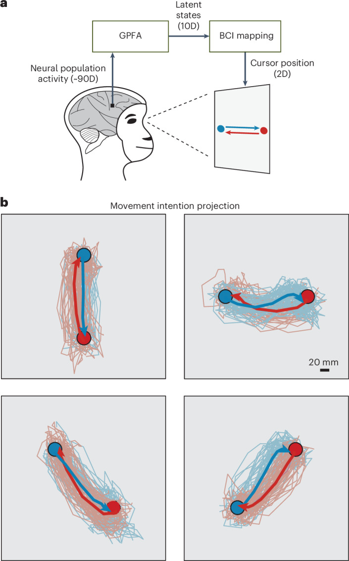
a, The BCI provides the monkey with moment-by-moment visual feedback of its population activity patterns as they evolve over time. We used a causal version of GPFA33 to estimate 10D latent states at each time step based on the recorded population activity (~90D). We then provided the monkey with visual feedback of two dimensions of its latent states (defined by a BCI mapping; Methods), which determine the moment-by-moment 2D position of the BCI cursor. The monkey moved the cursor from target A to target B (blue) and from target B to target A (red). b, Cursor trajectories for the four possible target pairs while using the MoveInt BCI mapping. For visualization, trajectories are colored by the start target (for example, red trajectories indicate movements originating at the red target and moving to the blue target). Thin traces represent individual trial trajectories. Thick traces represent trial-averaged trajectories. Note the high degree of overlap between the red trajectories and blue trajectories for each target pair.
A key experimental design choice is to specify which 2D projection of its 10D neural trajectories we show to the animal. Each experiment began with a BCI mapping that was intuitive to use and captured the monkey’s movement intention, that is, the ‘movement-intention’ (MoveInt) mapping (Methods). With the MoveInt mapping, the animals could move the cursor flexibly throughout the workspace. Animals performed a two-target BCI task in which they moved the cursor between a pair of diametrically opposed targets (that is, target A and target B). In the MoveInt projection, the cursor trajectories from target A to target B were highly overlapping with the cursor trajectories from target B to target A (Fig. 2b). The overlapping cursor trajectories might lead one to believe that, from a given position in 10D space, it would be possible to move in multiple different directions. That is, this projection makes it appear that the time courses of population activity patterns are flexible.
The MoveInt BCI mapping is just one 2D projection of the 10D space of neural population activity. Although the cursor trajectories between a given target pair overlap in the MoveInt projection, the neural trajectories are defined in a 10D space and need not overlap in all dimensions. In fact, when we view other projections of the 10D space, the temporal structure of the neural trajectories differs in a direction-dependent way (Fig. 3a). In some 2D projections, we found that the neural trajectories when moving the cursor from target A to target B were distinct from the neural trajectories when moving the cursor from target B to target A (Fig. 3b). These direction-dependent paths show that the monkey did not simply produce the same population activity patterns in a different ordering to move back and forth between the targets. Rather, neural activity followed different paths in 10D space that projected onto overlapping paths in the MoveInt projection. We identified a 2D projection that maximized the separation between the A-to-B and B-to-A trajectories, that is, the ‘separation-maximizing’ (SepMax) projection (Fig. 3c; Methods). The neural trajectories that are overlapping in the MoveInt projection are clearly separable in the SepMax projection (Fig. 3d and Extended Data Fig. 1a–c). Neural activity in the SepMax projection resembles that seen in studies of the motor cortex during reaching1 and is suggestive of underlying network constraints that govern the time courses of neural population activity.
Fig. 3. Neural trajectories follow direction-dependent paths in the 10D activity space.

a, The MoveInt mapping provides the monkey feedback of one particular 2D projection of the neural trajectories. In the MoveInt projection (indicated by the gray background), the A-to-B (blue) and B-to-A (red) trajectories overlap. However, when we examine the 10D space in which the neural trajectories reside, we find that the A-to-B (blue) trajectories are distinct from the B-to-A (red) trajectories. The SepMax projection is indicated by the light blue background. b, The SepMax projection is a 2D projection of the neural trajectories in which the A-to-B (blue) trajectories are distinct from the B-to-A (red) trajectories. Thin traces show trajectories for individual trials. Diamonds indicate the midpoint (Methods) for each trial. Thick traces represent trial-averaged trajectories. c, We quantify the separation between red and blue trajectories in 10D space as the discriminability (d′) of the blue and red midpoints. Computing d′ involves the separation of the means (dashed line) and the covariances (ellipses) of the trial-to-trial scatter (Methods). d, Across all experiments (n = 111), the neural trajectories are substantially more separated in the SepMax projection (d′ = 4.5 ± 1.6; mean ± s.d.) than they are in the MoveInt projection (d′ = 0.9 ± 0.6; mean ± s.d.; two-sided t test, P < 10−41). Means are indicated by the triangles.
Extended Data Fig. 1. Results hold for each animal individually.

a–c, Per animal results for Fig. 3d. For each animal individually, the neural trajectories are substantially more separated in the SepMax projection than in the MoveInt projection. a, Monkey E. SepMax d′ = 5.6 ± 1.2 (mean ± s.d.), MoveInt d′ = 0.9 ± 0.6 (mean ± s.d.; two-sided t-test, p < 10−5, N = 50). b, Monkey D. SepMax d′ = 2.9 ± 0.9 (mean ± s.d.), MoveInt d′ = 1.1 ± 0.8 (mean ± s.d.; two-sided t-test, p < 10−3, N = 40). c, Monkey Q. SepMax d′ = 4.7 ± 1.2 (mean ± s.d.), MoveInt d′ = 0.7 ± 0.4 (mean ± s.d.; two-sided t-test, p = 0.0035, N = 21). d–f, Per animal results for Fig. 6e,g,i. Distribution of the percent difference of the two initial angles (black; monkey E: 2.4 ± 15.4%, monkey D: 0.29 ± 28.5%, monkey Q: −7.6 ± 20.4%, mean ± std) illustrated in Fig. 6d. Zero percent difference (vertical dashed line, left) indicates that the cursor moves along the flow field before acquiring the intermediate target. One hundred percent difference (vertical dashed line, right) indicates that the cursor was able to move straight to the intermediate target (that is, against the flow field). For reference, the no-change distribution (dark red triangle and line; monkey E: −11.3 ± 33.0%, monkey D: 4.5 ± 10.5%, monkey Q: 13.3 ± 16.7%; mean ± std) and the full-change distribution (gray triangle and gray line; monkey E: 88.6 ± 30.9%, monkey D: 93.7 ± 13.7% monkey Q: 87.9 ± 26.7%; mean ± std) are shown here, computed separately for each monkey. For monkeys E and D, the change in initial angle in the intermediate-target task is not statistically different from the ‘no change’ condition (two-sided t-test; monkey E: p = 0.06, N = 28; monkey D: p = 0.6, N = 9), but is statistically different from the ‘full-change’ condition (two-sided t-test; monkey E: p < 10−15, N = 28; monkey D: p < 10−5, N = 9). For Monkey Q, the change in initial angle in the intermediate-target task is less than the ‘no change’ condition (two-sided t-test, p = 0.03, N = 13) and is statistically different from the ‘full-change’ condition (two-sided t-test, p < 10−7, N = 13). g–i. Per animal results for Fig. 7e. Distribution of the percent difference of the two initial angles (black; monkey E: 9.4 ± 30.9%; monkey D: 19.0 ± 13.7%; monkey Q: 26.4 ± 26.7%, mean ± std) illustrated in Fig. 7d. Also shown is the distribution for the no change control (red) and the distribution for the full-change control (gray), computed separately for each monkey. There is a small change in the initial angle of the trajectories compared to the ‘no change’ condition (two-sided t-test; monkey E: p = 10−3, N = 28; monkey D: p = 0.09, N = 9; monkey Q: p = 0.01, N = 13), but did not approach the ‘full-change’ condition (two-sided t-test; monkey E: p < 10−11, N = 28; monkey D: p < 10−4, N = 9; monkey Q: p < 10−5, N = 13).
Once we identified this temporal structure in motor cortex activity during BCI control, we tested the flexibility of the time courses of neural population activity with a progression of three increasingly stringent experimental manipulations. In each experiment, we first gave the animal visual feedback of the dimensions where temporal structure was evident (~100 trials). Next, we asked if the animal could produce population activity patterns in a time-reversed neural trajectory (~100 trials). Finally, we directly challenged the animal to follow a prescribed path through a 2D projection of the 10D neural population space (~500 trials).
In our first test of the flexibility of the time course of neural activity, rather than providing the monkey visual feedback of its neural trajectories in the MoveInt projection (Fig. 4a), we provided visual feedback in the SepMax projection (Fig. 4b). The animal performed the same two-target task, moving the BCI cursor between targets A and B, but now with feedback of its neural activity in a projection in which we had observed directionally dependent curvature of the neural trajectories (Extended Data Fig. 2). We wondered if, given this feedback, the direction-dependent paths would persist (Fig. 4c, possibility 1) or if the monkeys would instinctively straighten out the trajectories (Fig. 4c, possibility 2). In behavioral studies, both humans34–38 and animals39,40 tend to adjust their movements to straighten out visually curved cursor trajectories. We leveraged this behavioral tendency to test how flexible neural activity time courses are by showing animals their curved neural trajectories. If the monkeys straightened out their cursor trajectories, that would show that the time courses of neural activity are flexible in the 10D neural population space. However, if they do not straighten out their trajectories, that would be consistent with the possibility that activity time courses are obligatory.
Fig. 4. Direction-dependent paths of neural trajectories persist even when BCI feedback is given in the SepMax projection.

a,b, The BCI paradigm allows us to choose which 2D projection of the neural trajectories we provide the monkey as visual feedback. Rather than show the monkey the MoveInt projection (gray background) (a), we rotate the population activity space relative to the monitor to show him the SepMax projection (light blue background) (b). c, Under the SepMax projection, we tested if the direction-dependent paths observed during the MoveInt block would persist (possibility 1) or if the monkey would straighten out its cursor trajectories (possibility 2). d, Neural trajectories are similar whether the MoveInt or SepMax projection is used for feedback. When the monkey received visual feedback of the MoveInt projection (top row), the A-to-B trajectories (blue) overlapped with the B-to-A trajectories (red) in the MoveInt projection (top left; gray background). Black outline indicates the projection that provides the monkey with visual feedback on the monitor. Those same trajectories are distinct in the SepMax projection (top right; light blue background). When the monkey received visual feedback of the SepMax projection (bottom row), the trajectories continued to follow direction-dependent paths (bottom right; light blue background). Those same trajectories overlap in the MoveInt projection (bottom left; gray background). e, Same trials as shown in d (bottom right), separated into ‘early’ trials, that is, the first half (50 trials for this session, left), and ‘late’ trials, that is, the second half (49 trials for this session, right). f, We calculated d′ separately for the early trials and the late trials and computed to determine whether the animal straightened out its trajectories. As a reference, we also calculated for the same trajectories partitioned randomly into two groups. Across all experiments, the change in separation of ‘early’ versus ‘late’ trial trajectories ( = 0.07 ± 1.1, mean ± s.d.) was similar to that of the shuffle control ( = 0.01 ± 1.2, mean ± s.d.; two-sided t test, P = 0.69, n = 111). Means are indicated by the triangles. Example session indicated with circles.
Extended Data Fig. 2. BCI performance is similar regardless of the projection in which feedback is provided.

BCI performance with the SepMax mapping is similar to the performance with the MoveInt mapping. We quantified performance in the two-target task using (a) success rate and (b) target acquisition time. N = 222 targets (111 experiments, 2 targets per experiment). a, The animals are highly proficient at the two-target task with both mappings, nearly always performing at 100%. b, Average target acquisition times as the monkey used the MoveInt mapping (horizontal axis) and the SepMax mapping (vertical axis). The target acquisition time is the time it takes the monkey to move the cursor in step 2 of the two-target task (Methods) and is calculated separately for A-to-B and B-to-A movements. Each dot represents one target. Across all monkeys, the acquisition times with the MoveInt mapping were 507.8 ± 109.5 ms (mean ± standard deviation) and those with the SepMax mapping were 553.4 ± 188.1 ms.
When animals were given visual feedback in the SepMax projection, their cursor trajectories continued to show strong persistence of direction-dependent paths (Fig. 4d, bottom right), consistent with possibility 1 (in Fig. 4c). In fact, this manipulation resulted in little change to the neural trajectories—the trajectories in the SepMax projection when it was being viewed by the animal (Fig. 4d, bottom right) were similar to the trajectories in the SepMax projection when the animal was receiving feedback of the MoveInt projection, and the SepMax projection was unseen by the animal (Figs. 4d, top right, and 5b, quantification). This was also true for neural trajectories in the MoveInt projection (Fig. 4d, left column)—trajectories were similar in the MoveInt projection whether or not the animal was observing that projection. Providing animals feedback of their neural trajectories in the SepMax view did not lead the animal to straighten out the trajectories in that projection after ~100 trials (Fig. 4e,f), suggesting that animals did not have volitional control over the ordering of population activity patterns. This finding was highly consistent across sessions, as visualized in Extended Data Fig. 3 and as quantified next (Fig. 5).
Fig. 5. Neural trajectories are robust to which projection provides the visual feedback.

a, We used flow fields to compare activity time courses across conditions. We calculated a separate flow field for each target condition, that is, cursor movements from A to B (blue) and cursor movements from B to A (red), to capture how the neural trajectory unfolds from a given initial condition. The flow fields for each condition are plotted together to visualize the overall flow. Each panel corresponds to Fig. 4d. Length and direction of arrows indicate the average, observed cursor velocity as a function of position in the corresponding 2D space. Arrows are colored by the direction of the cursor movement, and the color saturation indicates the number of data points that contribute to the average. The flow fields in the SepMax projection when seen (black outline) and unseen (no outline) by the monkey were similar (comparison noted by the large light blue arrow). In contrast, the flow field in the SepMax projection differed from the flow field in the MoveInt projection (comparison noted by large black arrow). b, We quantified the similarities between the flow fields by calculating the mean squared difference of the corresponding flow field vectors (Methods). The flow fields in the SepMax projection were similar regardless of whether they were seen or unseen by the monkey (vertical axis, cf. large light blue arrow in a). For reference, we considered a case where the flow fields were different, namely for the two projections that we used to provide visual feedback to the monkey (horizontal axis, cf. large black arrow in a). Filled symbols indicate sessions where the flow field difference in the SepMax projection across the two feedback projections (vertical axis) was significantly smaller than the flow field difference between the different feedback projections (horizontal axis, two-sided Wilcoxon rank-sum, P < 0.05, 90 of 111 sessions—48 of 50 sessions for monkey E, 23 of 40 sessions for monkey D and 19 of 21 sessions for monkey Q. Paired t test P < 10−16, n = 111 sessions). Red dot indicates the example session shown in a.
Extended Data Fig. 3. The temporal structure in neural population activity is robust.

Shown are three representative example experiments from each of the three monkeys. The same nine example experiments are also shown in Extended Data Fig. 7. These experiments were selected to show a range of flexibility under the SepMax projection during the instructed path task. In addition, these experiments show different target pairs in order to characterize the temporal structure throughout the workspace. Trajectories are plotted in the MoveInt (gray background) and SepMax (light blue background) projections. Black outlines indicate that the monkey is viewing that projection. When a projection is unseen by the monkey, the subpanel does not have an outline. Same conventions as Fig. 4d.
To more thoroughly characterize the direction-dependent paths of the neural activity time courses, we used a ‘flow field’ analysis. Computed from the data, a flow field describes how neural trajectories unfold from any given location in neural population space. Here we computed the velocity of the neural trajectories as a function of position in a given 2D projection. We identified the flow fields for the MoveInt and SepMax projections in both the MoveInt and SepMax feedback conditions (Fig. 5a and Extended Data Fig. 4; Methods). We observed that the flow field in the SepMax projection was similar whether or not it was the projection viewed by the animal (Fig. 5a, blue arrow). By comparison, the flow fields in the feedback projections (that is, MoveInt projection with MoveInt feedback versus SepMax projection with SepMax feedback) were quite different (Fig. 5a, black arrow). To quantify these observations, we calculated the mean squared difference between the flow fields (Methods; Fig. 5b). The difference between the flow fields was smaller for a given 2D projection in different feedback conditions than it was between different 2D projections (Fig. 5b, the points lie below the diagonal). The robustness of the flow fields under different visual feedback projections supports the hypothesis that neural population activity is constrained to follow specific time courses.
Extended Data Fig. 4. Flow fields are highly consistent across feedback conditions in random 2D projections.

We used a flow field analysis to compare neural trajectories in different 2D projections. a, To determine a cursor trajectory flow field, we segmented the 2D workspace projection into a grid of 20 mm × 20 mm voxels. Dots indicate cursor positions at each time point for all trials (for the example session E20190719). Dots are colored by the start target (blue: start target A at left of workspace; red: start target B at right of workspace). b,c, The velocity for a given voxel is defined as the velocity () averaged across all time points with a cursor position () in that voxel. For visual clarity, we show the flow fields separately for each target condition (b: target A to target B; c: target B to target A). The orientation of the arrows indicates the direction and the length of the arrows represents the magnitude of the velocity. The color indicates the number of time points that contributed to the average. d–h, The flow field analysis (Fig. 5) shows that the time courses of neural activity are strongly constrained within the SepMax projection, regardless of whether the animal receives feedback of their neural activity in the MoveInt or SepMax projections. However, it is not yet clear whether these constraints are limited to specific subspaces or whether neural trajectories are constrained in other dimensions of the 10D space. To test this, we applied a flow field analysis similar to that used in Fig. 5 (Methods; a–c above) to neural activity in random 2D projections of the 10D space. We first projected neural trajectories into random 2D subspaces: where is a random matrix with orthonormal columns and is the latent state at time step as defined in equation (5). Then we estimated flow fields in this 2D subspace, using a 1 × 1 latent unit voxel size. d, ‘Other feedback’ comparison. We compared the flow fields in a given projection between feedback conditions. For example, in the SepMax projection we compared the flow field during MoveInt feedback (top) and the flow field during SepMax feedback (bottom). Note that the illustrated flow field comparison is the same as is shown in Fig. 5 for the SepMax projection (Fig. 5 light blue arrow), but we repeat the comparison for 400 random 2D projections per experiment to get the cyan distribution in g and h. In order to appreciate the amount of change we observe in the flow fields in the ‘other feedback’ comparison, we constructed control distributions for which we expect no change and maximal change in the flow fields. For a no-change distribution, we compared flow fields for different subsets of trials with the same visual feedback. We call this distribution ‘fixed feedback.’ For maximal change distributions, we constructed two distributions: one in which the flow fields are overlapping and maximally different, that is, the ‘time-reversed’ condition (e), and one in which the flow fields are different but less overlapping, that is, the ‘alternate-target’ condition (f). e, ‘Time-reversed’ comparison. In the time-reversed comparison, we compared the flow fields between trials for a given feedback condition, for example, MoveInt trajectories (top) to a time-reversed version of the MoveInt trajectories (bottom). We generated the time-reversed neural trajectories in an offline analysis by reversing the temporal sequence of trajectories , making the last time point the first and the first time point the last. Note that the schematic simply reverses the direction of the velocity vectors. f, ‘Alternate-target’ comparison. In the alternate-target comparison, we compared the A-to-B flow field to the B-to-A flow field for a given feedback condition. For example, we compared trajectories from one start target (top) to trajectories from the other start target (bottom) during MoveInt feedback. g, Quantification of flow field comparisons. We compared 400 random 2D projections per experiment for each flow field comparison. By comparing the difference in flow fields for the ‘other feedback’ comparison to these three control distributions across random projections, we can determine whether the feedback provided to the monkeys changed neural trajectories in the full 10D space. For each experiment, we compare the flow fields of 50 random trial splits in each of the 400 random projections. The total number of available trials for a given start target condition (49 ± 3.8 trials) was randomly sub-selected to form two sets of 20 trials and flow fields were estimated for each set. All comparisons were between flow fields for each set of trials (except for the fixed feedback case which compared flow fields between sets of trials for a given trial split). We calculated the mean squared difference between velocity vectors of corresponding voxels of the flow fields and took the median of those values across voxels (Methods) for each of the random trial splits in each projection. For the jth projection, we quantified the flow difference, , as the mean across trial splits of the median values. To compare these distributions across experiments, we normalized the flow difference with respect to the fixed feedback as the lower limit, and time-reversed as the upper limit , where is the normalized flow field difference for jth projection, is the flow difference for the jth projection, and are the per experiment average across projections of the flow difference magnitude for the fixed feedback and time-reversed distributions, respectively. A indicated that there was no change in flow difference magnitude between conditions, while indicated that flow difference magnitudes were maximally different between comparison conditions. We averaged across projections to yield a single value, , for each experiment. By definition, for the Fixed feedback comparisons and for the Time-reversed comparisons. We found that the flow difference for the other feedback comparisons was small. The other feedback (cyan) comparison was not significantly different from the fixed feedback (gray) comparison (paired t-test, p = 0.0934). h, We also measured ‘flow field overlap’, which quantifies the degree to which the trajectories occupy the same region of state space. Flow field overlap, was quantified as the number of voxels with a minimum of 2 time points within that voxel for each of the flow fields being compared. Like the flow difference metric, we calculated the flow field overlap of 50 random trial splits for each of the 400 random projections. To compare these distributions across experiments, we normalized the flow field overlap with respect to the fixed feedback comparison, which has the highest degree of observed flow field overlap , where is the normalized flow field overlap for jth projection, is the flow field overlap for the jth projection and is the per experiment average across projections of the overlapping voxels for the fixed feedback distributions. A indicates that the region of the state space occupied by the trajectories was highly non-overlapping between distributions, while indicates that the overlap between trajectories was the same as the amount of overlap observed in the fixed feedback condition. We averaged across projections to yield a single value, , for each experiment. We found that the fixed feedback, other feedback and time-reversed comparisons all show high flow field overlap, although the flow field overlap for the fixed feedback comparison was significantly larger than the other comparisons (paired t-test, p < 0.001). If the neural trajectories are constrained in the 10D space, the other feedback flow field comparisons should have low flow difference (similar to that for the fixed feedback comparison) and high flow field overlap (similar to that for the fixed feedback and time-reversed comparisons). Taken together, these results indicate that neural flow fields and the resulting neural trajectories are highly consistent in all dimensions, regardless of the visual feedback provided to the animal.
We wondered whether these temporal constraints were present only in specific subspaces or whether the time courses of neural activity were also constrained in other dimensions. We found that the time courses of neural activity are highly consistent in other dimensions, regardless of the view provided to the animal (Extended Data Fig. 4). This indicates that the robustness of the temporal structure captured by the SepMax projection is not unique. It is worth noting that the time courses of neural activity are highly flexible in the dimensions of the MoveInt projection (cf. Fig. 2b), even while being constrained in the higher dimensional space.
The persistence of the characteristic paths of the neural trajectories enables an additional demonstration of the robustness of the temporal structure. In a separate set of experiments, we provide the monkey feedback of its neural trajectories in the SepMax projection in one block of trials and the ‘reflected’ SepMax projection in a separate block of trials. We leveraged the fact that we can reflect the orientation of the identified SepMax projection about the axis that connects the targets (Extended Data Fig. 5a). This manipulation changes the direction-dependent trajectory curvature. For example, if the cursor trajectories from target A to B curved upwards in the SepMax projection, the trajectories curve downwards in the reflected-SepMax projection. With feedback in the reflected-SepMax projection, one possibility is that the cursor trajectories might continue to exhibit the same direction-dependent trajectory curvature that we observed before the reflection (Extended Data Fig. 5b, possibility 1). This possibility would demonstrate flexibility in the activity time courses and would indicate that perhaps the animal simply had a preference for generating population activity patterns along particular paths. Another possibility is that the cursor trajectories might show the corresponding reflection of the characteristic paths in the reflected-SepMax projection (Extended Data Fig. 5b, possibility 2). This possibility would be consistent with a rigid temporal structure. Consistent with possibility 2, when we provided the monkey feedback of its neural trajectories in the reflected-SepMax projection, the cursor trajectories were also reflected (Extended Data Fig. 5c,d). This observation further strengthens our finding of a robust temporal structure that likely reflects network constraints.
Extended Data Fig. 5. Temporal structure is robust to reflection of the workspace.

We assessed if the activity time courses indicated underlying network constraints or just a preference of the monkey. a, By construction, the SepMax projection is unique up to a reflection about the target axis (Methods). In a separate set of 18 experiments, we presented the animal with both reflections of the matrix (equation (13)). To do this, we reflected the orientation of the identified SepMax projection about the target axis to produce a ‘reflected-SepMax’ mapping. We then provided the reflected-SepMax mapping as feedback to the monkey. b, If the observed temporal structure arose from a visual preference for curvature in a particular direction, the trajectories under the reflected-SepMax feedback would continue to show the structure observed in the SepMax projection (possibility 1). However, if the trajectories arose from underlying network constraints, the trajectories under the reflected-SepMax feedback would also be reflected (relative to the SepMax trajectories; possibility 2). c, Flow fields from an example experiment during BCI control using both SepMax and reflected-SepMax mappings. Cursor trajectories are shown as insets. The SepMax projection was identified from the neural activity generated while the animal was receiving visual feedback in the MoveInt projection (left). The animal was provided visual feedback of the SepMax projection (center) and the reflected-SepMax projection (right). We observed that the orientation of the cursor trajectories under the reflected-SepMax feedback was reflected relative to the trajectories under the SepMax feedback, consistent with possibility 2. d, The flow fields indicated that the trajectory curvature arises from underlying network constraints rather than the animal’s visual preference. We calculated the difference between the flow fields (Methods) in the SepMax projection and the reflected-SepMax projection (comparison noted by large red arrow in c). As a benchmark for similar flow fields, we calculated the difference between the flow fields in the SepMax projection during MoveInt and SepMax feedback (comparison noted by large light blue arrow in c). The difference between the flow fields in the SepMax and reflected-SepMax projections (horizontal axis) was significantly larger than the difference between the flow fields of the SepMax projection in the MoveInt and SepMax feedback conditions (vertical axis; 18/18 experiments two-sided Wilcoxon rank-sum test, p < 0.001). The example session shown in c is indicated by a red dot.
Taking stock, we first observed temporal structure in dimensions of neural population activity that were unseen by the animal during BCI control (Fig. 3). When we provided visual feedback of those dimensions to the monkey, the characteristic time courses of neural activity persisted (Fig. 4 and Extended Data Fig. 5). In our second test, we sought a more direct test of the flexibility of neural trajectories. We asked if the animal could produce previously observed population activity patterns in a time-reversed ordering. To do this, we used the empirically derived flow fields (Fig. 5) to describe the neural trajectories in the SepMax projection (Fig. 6a). Then, we challenged the animal to move the BCI cursor against the flow field (Fig. 6b, large red arrow). We presented a target along one of the paths of the flow field (Fig. 6c). This ‘intermediate target’ (IT; black target) was naturally acquired from target A (that is, the blue path from target A to the IT follows the flow field), but moving the cursor from target B (that is, red target) to the IT challenged the monkey to order its population activity patterns into a neural trajectory that would move against the flow field. Notably, the animal was not asked to generate new population activity patterns but rather to generate previously observed patterns in a new order. When the monkeys moved the cursor from target B to the IT, they did not generate the time-reversed neural trajectory to move directly to the IT against the flow field. Rather, they acquired the target by initially following the path of the flow field and then hooking back toward the IT (Fig. 6c, black traces). To succeed at the IT task, the animals did not violate the flow field but instead, at least initially, followed the flow field.
Fig. 6. Challenging monkeys to violate the flow field.

a, Flow fields (small arrows) characterize the distinct paths (large arrows) as the monkey moves the cursor from A to B (blue) and B to A (red). b, We sought to assess if the monkey could produce a trajectory that moves against the flow field. c, To challenge the monkeys to move against the flow field, we placed an intermediate target (IT; black circle) along the path of the flow field. Black lines represent single-trial cursor trajectories (thin lines) and the trial-averaged cursor trajectory (thick line) to the IT. d, To quantify the animal’s ability to move the cursor against the flow field, we measured the initial angle between the trajectory to the IT (black line) relative to the direct path to the IT (dashed line). For comparison, we measured the initial angle between the cursor trajectory to the blue target in the two-target task (red line; cf. Fig. 4d) and the direct path to the IT. e, Distribution of the percentage difference of the two initial angles illustrated in d across experiments. A 0% difference (vertical dashed line, left) indicates that the cursor moves along the flow field before acquiring the IT. A 100% difference (vertical dashed line, right) indicates that the cursor was able to move straight to the IT (against the flow field). The percentage difference is not statistically different from zero (two-sided t test, P = 0.84, n = 50). f, For the ‘no change’ control, we compute the initial angles between the early (red line, same as in d) and late (dashed red line) two-target trials relative to the direct path to the IT (dashed black line). g, ‘No change’ distribution across experiments. This distribution is not statistically different from zero (two-sided t test, P = 0.61, n = 50). h, For the ‘full-change’ control, we show the first nine time points of trial-averaged center-out cursor trajectories under the MoveInt projection (cf. Fig. 2b). We measured the initial angle relative to the direct path to the cued target (dashed line for the example shown) for trajectories to the cued target compared to trajectories to the neighboring +45° and −45° targets. Here we highlight the initial angles for the blue trajectory (cued target) and the aqua trajectory (−45° target). i, ‘Full-change’ distribution across experiments. The distribution is statistically different from zero (two-sided t test, P < 10−28, n = 50) and from 100% change (two-sided t test, P = 0.008, n = 50).
We sought to understand to what extent the trajectories during the IT task follow or violate the flow field defined by the two-target trajectories (Fig. 6a). We asked if the initial part of the cursor trajectories in the IT task (Fig. 6d, black arrow) were more similar to the cursor trajectories in the two-target task (Fig. 6d, red arrow) or the time-reversed, direct path (Fig. 6d, black dashed line). We defined the initial angle of the cursor trajectories of both tasks with respect to the time-reversed direct path. Then we calculated the difference in the initial angle between the two-target trajectories and the IT trajectories (Fig. 6e; Methods). Across experiments, there was no systematic difference in the initial angle for the IT trajectories relative to the two-target trajectories (−0.56 ± 19.61%; mean ± s.d.; t test, P = 0.84, n = 50; see Extended Data Fig. 1d–f for animal-specific results). To interpret this, we computed reference distributions corresponding to a ‘no change’ condition and a ‘full-change’ condition. In the ‘no change’ condition (Fig. 6f,g), we computed the difference in the initial angle for two partitions of the two-target trials. In this condition, there is no difference in the trajectories (Fig. 4e,f). By contrast, the ‘full-change’ condition (Fig. 6h,i) captures the amount of change we observe under the MoveInt projection where the animal can flexibly move the cursor from the same starting position to multiple targets. The change in initial angle in the IT task (Fig. 6e) is not statistically different from the ‘no change’ condition (Fig. 6g; t test, P = 0.78) but is statistically different from the ‘full-change’ condition (Fig. 6i, t test, P < 10−27). This indicates that activity time courses are not readily modified.
With the experimental manipulations described thus far, we observed only minimal modification of the cursor trajectories. However, those tasks did not require that the animals generate the time-reversed neural trajectory for success. The possibility remains that the animals can modify their neural trajectories, but they were not sufficiently incentivized to do so. In our third test, we imposed a visual boundary around the time-reversed trajectory (Fig. 7a). This ‘instructed path task’ constrains the path that neural activity can take to the IT41. We gradually reduced the size of the boundary to approach the direct path to the IT, which represents the time-reversed neural trajectory (Extended Data Fig. 6; Methods). Notably, the allowable path includes the population activity patterns that comprised the previously observed neural trajectories. This means that we know that the animal can produce each of the required population activity patterns, but this task challenges the animal to produce them in a different order. If the animal can produce the time-reversed neural trajectory, the cursor will move directly to the IT. If the animal cannot alter the time course of its population activity patterns, then it will not be able to succeed at the task.
Fig. 7. Monkeys did not generate time-reversed neural trajectories.

a, The monkeys performed an ‘instructed path task’, in which they had to move the cursor from the start target (red circle) to the IT (black circle) without exiting a visual boundary (oval outline). b, To encourage the monkeys to modify their trajectories, we incrementally reduced the size of the boundary so that an inability to alter their trajectories would eventually lead to a failure at the task. Cursor trajectories for the least and most restrictive paths for an example session. The least restrictive path (left) minimally affected the cursor trajectories relative to the unconstrained trajectories (cf. Fig. 6c). With the most restrictive path, the animal only succeeded approximately half the time (right). Successful trials are shown as thin black lines. Failed trials are shown as thin red lines. The thick black line shows the average of all trials, regardless of success, for that boundary size. c, The five boundary sizes (oval outlines in different shades of gray; size refers to the distance of the boundary from the target indicated by the dashed line) and trial-averaged cursor trajectories of successful trials only for each boundary size (line in corresponding shade of gray) for the example session. d, Comparison of the initial angle of the most constrained trials (trial-averaged trajectory of all initiated trials regardless of eventual success, black line) to the initial angle of the two-target trials (trial-averaged trajectory of all initiated trials regardless of eventual success, red line; same as in Fig. 6d,f). We calculated the initial angles relative to the direct path (black dashed line) from the start target (red circle) to the IT (black circle). e, Distribution of the percentage difference in initial angle across experiments (n = 50). The mean is indicated by the black triangle. For reference, the no-change distribution (dark red triangle and line; mean ± s.d.) and the full-change distribution (gray triangle and line; mean ± s.d.) from Fig. 6 are shown here.
Extended Data Fig. 6. Example of an instructed path experimental session.

Animals were instructed to move their BCI cursor from the red target to the black ‘intermediate’ target while keeping the cursor within the visual boundary. For reference, the blue circle indicates the location of the other target in the two-target task but was not shown to the animal in this task. To encourage the animals to modify their trajectories, we gradually decreased the size of the boundary diameter over the course of each experiment. a, Cursor trajectories for individual trials (thin traces) and averaged across trials (thick traces) to the intermediate target (black circle) during unconstrained trials (far left) and in the presence of visual boundaries of decreasing diameters (from left to right). The average cursor trajectory includes all initiated trials, regardless of success. As the size of the boundary is reduced, the qualitative structure of the trajectories does not change. b, Success rate over the course of an instructed path experiment. Every 25 trials, we checked to see if the success rate was greater than the predetermined threshold (dashed line). If so (green dots), the boundary was reduced in size. If the animal failed to meet the success rate threshold (red dots), the size was maintained for an additional block of 25 or 50 trials (Methods). This procedure was continued for a minimum of 500 trials. We compared the observed (thick black) success rate in response to the visual boundary to the predicted (thin red) success rate, computed by applying the same boundaries to the unconstrained trial trajectories. The observed success rate was greater than the predicted success rate, indicating that the animal was responding to the boundary but was unable to change the initial angle of the cursor trajectory (thick traces in a).
Even in this task with a strong incentive to produce time-reversed trajectories, animals only minimally modified their trajectories as we reduced the size of the boundary. Instead of modifying their trajectories, they began to fail at the task (Fig. 7b, compare left and right). Across all sessions, we did not observe cursor trajectories that went directly to the IT, although the animal was previously able to generate each population activity pattern along that path. Rather, the trajectories continued to follow the natural direction of flow, showing the hook-like bowing feature (Fig. 7b,c; see Extended Data Fig. 7 for more example sessions) that we observed in the IT experiment (Fig. 6c).
Extended Data Fig. 7. There is minimal flexibility in the cursor trajectory when monkeys are directly challenged to follow an instructed path.

Here we show trial-averaged cursor trajectories for successful instructed path trials for the same experiments as in Extended Data Fig. 3. Experiments are ordered from less flexible (left) to more flexible (right). Flexibility is quantified using the initial angle metric (Methods). Starting target locations are shown in red or blue, and intermediate targets are shown in black. Trial-averaged cursor trajectories are plotted for each boundary size (same convention as Fig. 7c). The change in the initial angle is minimal over the course of an instructed path experiment, even in the ‘more flexible’ experiments (cf. Fig. 7). The initial angle does not approach the direct path to the intermediate target.
To quantify the flexibility of neural trajectories, we again used the ‘change in initial angle’ metric. We examined the initial angle of the trajectories in the presence of the most restrictive boundary in comparison to the two-target trials (Fig. 7d). Across experiments, there was a small (15.5 ± 20.3%; mean ± s.d.) change in the initial angle of the trajectories compared to the ‘no change’ condition (Fig. 7e; t test, P < 10−5, n = 50; see Extended Data Fig. 1g–i for animal-specific results). As in the IT task (Fig. 6d,e), during the instructed path task, the monkeys produced trajectories that were more similar to the two-target trajectories than the direct path (Fig. 7d,e; t test, P < 10−20, n = 50). That is, the animals produced cursor trajectories that followed the flow field, despite the presence of the boundary compelling them to alter their trajectories. This lack of flexibility demonstrates that strong constraints exist on the time courses of neural activity.
Finally, we considered whether the animals simply did not understand the instructed path. Arguing against this interpretation, the animals performed better at the instructed path than predicted from applying the boundaries to the unconstrained trials (Extended Data Fig. 6b). This shows that they were attempting to respond to the presence of the boundary. Even with these small changes in behavior, the trajectories exhibited in the instructed path task continued to resemble the direction-dependent curvature of the unconstrained trajectories.
Discussion
Here we assessed the flexibility of the dynamical structure present in neural population activity. We first observed the naturally occurring time courses of neural population activity in the motor cortex during BCI control. We found that these time courses exhibited rich temporal structure while monkeys used a BCI, reminiscent of what is seen in the motor cortex during reaching1 and elsewhere in the cerebral cortex during other behavioral tasks2,5–7,11,24. This temporal structure persisted when animals were given visual feedback of their neural population activity in projections that make the temporal structure most evident. When challenged to generate time-reversed versions of naturally occurring time courses, animals did not do so, even when strongly incentivized. These results indicate that the temporal structure of neural population activity that we, and others (for example, refs. 1,2,5–7,11–13), have observed likely reflects underlying network constraints that are difficult to violate.
Why should neural activity exhibit temporal structure? Temporal structure, often referred to as neural dynamics, is taken as a signature of the computation carried out by the network of neurons23. This understanding of temporal structure in neural population activity originated in neural network modeling studies17,18,22, in which the time evolution of activity within a network is shaped by the connectivity of the network, and embodies the computation being performed. Once provided with an input, the network evolves from its initial activity state to a final activity state to carry out a computation (for example, a commitment to a decision, a plan for a specific movement or the execution of a movement). Examples of temporal structures include the flow of activity toward a point attractor, line attractor or a stable limit cycle. Empirical studies have demonstrated that such temporal structures may underlie arm movements1, olfaction2, sensory perception3,4, decision making5–8, timing11,12 and more. By showing that the temporal structure in neural population activity is not easy for animals to violate using volitional control, our work provides causal evidence that the neural activity time courses observed in those studies are not arbitrary but instead likely reflect the underlying network connectivity that gives rise to the relevant computations.
In network models, activity is a function of both the connectivity of the network and the inputs to the network. Thus, changing the temporal structure in the activity of a network would require altering the network’s connectivity or altering its inputs. M1’s population dynamics have been shown to depend on the inputs to M1, for example, from the thalamus and other brain areas42–45. It is well known that monkeys can volitionally alter activity in the brain areas that provide inputs to M1. For example, the activity in the premotor cortex that leads to a reach to the right is different from the activity that leads to a reach to the left46. Similarly, in the BCI tasks described here, changes in the inputs to M1 occur to move the BCI cursor in different directions. Such changes to the inputs likely drive rapid learning in sensorimotor adaptation tasks47,48. In our experiments, animals were free to change the inputs to M1 as they tried to alter the natural time course of their neural activity. That animals did not alter the natural activity time courses may indicate that there are limits on the extent to which inputs can change population dynamics49. This may be because inputs can only influence certain dimensions of M1’s population activity (which include the dimensions of the MoveInt projection in our study) or that the strength of inputs cannot overcome M1’s intrinsic dynamics. In addition, our results indicate that any learning mechanisms that might have been engaged during this task were unable to adjust M1’s local connectivity sufficiently to alter the natural activity time courses, at least on the 1–2 h time scale of our experiments. These considerations suggest that M1’s dynamical structure is highly conserved and not readily changeable, implying that these dynamics serve important functions that the brain seeks to preserve.
This study demonstrates the power of BCIs as a tool to probe neural population dynamics. BCIs allow us to place specific requirements on neural population activity directly, whereas experiments relying on arm or eye movements indirectly challenge the properties of neural activity. It might be a concern that the BCI paradigm itself somehow contributed to the apparent inflexibility of the neural trajectories. For example, the motor cortex receives inputs about arm posture and the movement goal that influences the population activity. In our BCI experiments, the animal’s arms were restrained in a particular posture throughout the task. By ensuring that the arm posture was constant over time (cf. Extended Data Fig. 7), we were able to emphasize the characterization of the intrinsic dynamics of M1. If we had allowed the arm to move, M1 would have received time-varying postural inputs, which would have made the task of characterizing the intrinsic dynamics of M1 more difficult.
Other reasonable concerns include that the animals were not sufficiently motivated to modify their trajectories or that they did not understand the task. We consider these explanations unlikely because these well-trained and highly motivated animals persisted in the face of challenging tasks, even when they involved hundreds of trials with low success rates. The animals showed some modest improvements in task success (Extended Data Fig. 6), which speaks to their motivation to perform the task, but these improvements did not reflect flexible control of their activity time courses (Fig. 7). Furthermore, these small improvements indicate that the animals understood what was asked of them but were nevertheless unable to alter the temporal structure of their neural population activity on the time scale of ~500 trials.
The temporal structure we find here (cf. Fig. 3) is reminiscent of the rotational dynamics shown in ref. 1 during arm movements. Subsequent studies showed that reversing the kinematics of the hand is not sufficient to reverse the direction of those rotational dynamics50. Here temporal structure is evident without arm movements. This indicates that the temporal structure is not merely a reflection of descending motor commands or sensory (for example, proprioceptive) feedback but instead is an intrinsic property of the network. One of the key features of M1 population dynamics is that it exhibits low ‘tangling’51. This is taken as evidence of a first-order dynamical system, where the activity moves in a direction defined by the current activity state. Our study strengthens those findings because we challenged the animals to move their neural activity in a manner that would have resulted in high tangling, but they did not do so. Instead, the neural activity continued to move in directions of low tangling. Although we find that the time courses of neural activity are highly constrained in the overall population activity space, it is interesting that there exists a subset of dimensions (in our study, the MoveInt projection) in which the population activity appears to be able to flexibly move along any path (cf. Fig. 6h). This supports a key idea underlying the computation through the dynamics framework—that fixed dynamics (seen in ‘output-null’ dimensions) can give rise to a broad range of different outputs (seen in ‘output-potent’ dimensions).
In our previous work, we have examined which population activity patterns monkeys can readily produce31,48,52 and demonstrated how new population activity patterns that support new behaviors can emerge with extensive training32. This study extends our previous findings by addressing the temporal structure of neural population activity. The present work shows that neural activity is even further constrained than reported in earlier BCI studies—not only is neural activity constrained by an intrinsic manifold31 and neural repertoire48, but we now show there are temporal constraints on neural population activity that are difficult to violate. It might have been the case that animals could produce any neural trajectory within the intrinsic manifold, but that is not what we observed. It remains a possibility that with more time or practice, perhaps using incremental training32, animals might learn to alter the temporal structure of their neural population activity. This process would presumably require altering the connectivity within M1 and/or how M1 is controlled by other parts of the brain. Another intriguing possibility is that even with extensive training, temporal structure would still persist. By this view, behavioral flexibility might be achieved by flexibly combining fixed dynamical motifs53,54, rather than by forging new dynamics.
Methods
Electrophysiology and behavioral monitoring
All animal procedures were approved by the University of Pittsburgh Institutional Animal Care and Use Committee in accordance with the guidelines of the US Department of Agriculture, the International Association for the Assessment and Accreditation of Laboratory Animal Care and the National Institutes of Health. Data collection was performed using LabVIEW (2014) and MATLAB (2024a). Three animals were trained on a center-out reaching task. We then implanted arrays in the motor cortex contralateral to the trained reaching arm. We recorded neural activity from the proximal arm region of the primary motor cortex (M1) in two male rhesus macaques (monkey E, aged 12 years; monkey D, aged 12 years) using a 96-electrode (1.0 mm electrode length) microelectrode array (Blackrock Microsystems). In a third monkey (monkey Q; male, aged 6 years), we implanted a 64-electrode (1.0 mm electrode length) array in the dorsal premotor cortex and a 64-electrode (1.5 mm electrode length) array in M1. The recorded neural signals were amplified and digitally processed using the TDT RZ2 system (Tucker–Davis Technologies). The digitized signals were bandpass filtered between 300 Hz and 3 kHz. We recorded neural activity as threshold crossings, where a threshold crossing was detected when the depolarizing phase of the voltage signal crossed a threshold of three times the root-mean-square (RMS) voltage. We estimated the RMS voltage of the signal on each electrode before each experiment while the monkeys sat calmly in a darkened room. We recorded 94.0 ± 1.1, 79.9 ± 1.6 and 96.7 ± 0.5 neural units (mean ± s.d.) from monkeys E, D and Q, respectively. This study was conducted between 8 and 18 months after array implantation for monkey E, 9 and 18 months after implantation for monkey D and 3 and 6 months after implantation for monkey Q.
During experiments, animals sat head-fixed (monkeys E and D) or head-free (monkey Q) in a primate chair in front of a visual display with both arms loosely restrained in a pronated posture. To reduce hand movements during the BCI trials and to ensure a consistent hand position, the monkeys placed their hand (contralateral to the array) on a horizontal ‘touch bar’. The touch bar was instrumented with either a contact sensor (Spectra Symbol; some sessions with monkey E) or a force transducer (monkeys E, D and Q; Mini40, ATI Industrial Automation, NC) to measure hand contact with the touch bar. Animals were required to maintain this contact throughout the trial. Releasing the bar or exerting force outside of a predetermined window resulted in an immediate failure of the trial. The target force window was calibrated relative to the weight of the animal’s hand resting on the force bar independent of any task condition. The size of the force window depended on the orientation of the touch bar with respect to the 6-degree-of-freedom torque cell. Monkeys E and D maintained a force within an 11.8 N window, and monkey Q maintained a force within a 1.3 N window. For all monkeys, we could measure very small changes in force. The position of the hand was tracked using an LED marker (Phasespace). Consistent with previous BCI experiments31, there was minimal arm movement or force production during BCI trials (representative session shown in Extended Data Fig. 8).
Extended Data Fig. 8. Arm movements are minimal during BCI cursor control.

Here we show one representative example session for each of three tasks. a–c are from this study; d,e and f–h are included for comparison. d–h show data from the same monkey (monkey E), but from experiments not analyzed elsewhere in this paper. a, Example cursor trajectories during a two-target BCI task. b, Hand position as a function of time for the two-target BCI trials shown in a. Same vertical axis scale as in e and g. c, Force produced at the touch bar during the trials shown in a. d, Example of hand positions during a center-out reaching task. e, Hand position as a function of time for the center-out reaching task trials in d. Note that changes in hand position during BCI trials (b) are substantially smaller than those observed during center-out reaching trials. f, Example force trajectories during an isometric force task. For the isometric force task, the monkey applied force to the touch bar. We mapped the exerted force to cursor kinematics, allowing the monkey to acquire force targets. g, Hand position as a function of time for the isometric force task trials shown in f. h, Force as a function of time for the isometric force task trials shown in f. Forces exerted on the force bar during BCI control (c) were negligible when compared to those exerted on the force bar during the isometric force task. These observations are consistent with previous work31, in which we observed minimal arm movement during BCI tasks.
Behavioral tasks
For all behavioral tasks, trials were initiated by holding the touch bar for 250 ms. Upon initiation, a BCI cursor and a target were displayed simultaneously on the monitor. The cursor remained fixed at the center of the workspace for 500 ms (referred to as the ‘freeze period’), after which the cursor was placed under neural control. For all tasks, the animals were trained to move the cursor to acquire the presented target. The target was acquired when the cursor contacted the target (that is, no hold time was required). Animals received a liquid reward upon successful completion of a trial. Each animal performed the following BCI tasks, described in detail below—center-out task, two-target task, grid task, IT task and instructed path task.
Center-out task
Animals were required to move the BCI cursor from the center of the workspace to one of eight possible peripheral targets 90 mm from the center, arranged around a circle at 45° intervals. Animals were given 4 s to acquire the peripheral target. Failure to acquire the target within this time or failing the touch bar conditions (that is, releasing the bar or exerting force) resulted in a 2 s (monkeys D and Q) or a 5.5 s (monkey E) timeout. Targets were presented in a pseudorandom order such that each of the eight targets was presented and attempted once before any target was repeated. We used a block of 160 trials of the center-out task to calibrate the MoveInt decoder (see below).
Two-target task
Animals moved the BCI cursor to sequentially acquire two diametrically opposed peripheral targets (A and B). There were the following four possible target pairs: 0° and 180°, 90° and 270°, 45° and 225°, 135° and 315°. One target pair was tested in each session and was selected before the start of the session. These peripheral targets were placed 90 mm from the center of the workspace. There were nine experiments in which monkey Q was unable to acquire the peripheral targets at 90 mm, so we reduced the target distance to the greatest distance that the animal could acquire (80–85 mm). This task consisted of two steps. In the first step, the cursor and a peripheral target (pseudorandomly chosen to be target A or target B) simultaneously appeared on the screen, and the monkey had 4 s to acquire the target (Extended Data Fig. 9a, left). We refer to the target acquired in step 1 as the ‘start target’. In the second step, the diametrically opposed target appeared, and the monkey had 4 s to move the cursor from the start target to it, that is, from target A to target B or from target B to target A (Extended Data Fig. 9a, right). The trial was a success if the target in step 2 was acquired. Failing to acquire the second target led to a 5.5 s penalty, and all other failure modes resulted in a 2 s (monkeys D and Q) or a 3 s (monkey E) penalty.
Extended Data Fig. 9. Two-target task, grid task and intermediate-target task.

For each task, there are four possible orientations for the target pair: left–right (illustrated), up–down and both diagonals. a, Two-target task. The two-target task consists of two steps. In step 1 (left), the monkey moved the cursor (small black circle) to a peripheral target (blue circle). Upon completing step 1, step 2 (right) ensued. The monkey moved the cursor to the diametrically opposed target (red circle). There were also trials with the other ordering (that is, red then blue, not pictured). In each session, the same target pair was used throughout. b, Grid task. Step 1 for the grid task is the same as that for the two-target task (a, left). For step 2, there were three possible target locations: the diametrically opposed target (blue or red circles) or two targets perpendicular to the main target pair (black and gray circles). The probabilities of the targets were weighted so that for a given start target there were 50 trials to the diametrically opposed target and 10 trials to each of the other two targets. c, Determination of target position for the intermediate-target task. The monkey first acquired target A or target B (blue and red circles) and then was presented with an intermediate target (open black circles). The location of the intermediate target started at the center of the workspace (gray ‘+’), and we gradually increased the distance from the center in increments of 10% of the distance to the peripheral target (open black circles) until the success rate began to decline. Then, we slightly reduced the distance to ensure that the final position of the intermediate target (shaded black circle) was as close as possible to the path defined by the blue arrow, but that it could be acquired from both start targets.
Grid task
This variant of the two-target task included additional targets for the second step. Starting with the same peripheral target pair as was used for the two-target task in that session, the animal first acquired one of the two start targets, selected pseudorandomly. For the second step, there were three possible target locations—the diametrically opposed target or two targets orthogonal to the target pair axis (Extended Data Fig. 9b). The probabilities of the targets were weighted so that there were 100 total trials to the diametrically opposite target and 20 total trials to each of the other two targets. For each step, the animal had 4 s to acquire the target. Following the successful completion of the second step, the animal received a liquid reward. Penalty durations were as described for the two-target task.
IT task
This task was a variant of the two-target task in which the second step was to an IT, placed along an axis orthogonal to the target pair axis (Fig. 6). The location of the IT was selected for each experiment so that the animal could acquire it from both target A and target B (Extended Data Fig. 9c). To determine the excursion of the IT, we gradually increased the target distance from the center of the workspace in 10% increments of the peripheral target distance until the success rate began to decline. The final IT position was chosen to ensure both of the following: (1) the target location was aligned with the path of the flow field (Extended Data Fig. 9c, blue arrow) and (2) the success rate was high from both start targets. Across experiments, this procedure resulted in an IT position that was 31.2 ± 11.4 mm from the center of the workspace. The animals performed ~100 total trials (100.1 ± 0.3) of the IT task, moving from either start target to the IT (that is, A to IT and B to IT). These trials were used to estimate trajectory flexibility (‘Initial angle metric’).
Instructed path task
We modified the IT task so that the objective was to move the cursor along a path specified by a visual boundary around the start target and the IT (Fig. 7a). To succeed at the task, the animals were required to keep the cursor within the boundary as they acquired the IT. The boundaries were straight, capped cylinders that encased the allowable paths between the start target and the IT. The boundary edges were equidistant (ranging from 30 to 150 mm) from the target axis (that is, the line that connects the targets).
A trial of the instructed path task began with the presentation of the start target. After its successful acquisition, the IT and the visual boundary appeared simultaneously. Animals then had 4 s to acquire the IT (that is, the ‘acquire time’) without the BCI cursor touching the boundary to receive a reward. Failing the boundary requirement resulted in a time penalty that was 2 s plus the remaining acquire time. This trial structure ensured that animals would receive shorter time penalties for trials in which they were actively attempting to acquire the target and longer penalties for failing quickly.
The instructed path task started with a boundary size that required minimal modification of cursor trajectories for success. The first boundary was chosen to have a width of 110 or 120 mm, except for one session for monkey D (150 mm width) and two sessions for monkey E (80 mm width). Then, we gradually reduced the size of the boundary to encourage the animals to modify their cursor trajectories. The reduction happened in one of two ways. For all sessions with monkeys E and D, and 6 of 13 sessions with monkey Q, we evaluated the animal’s task performance every 25 trials and reduced the boundary’s width by 10 mm if the animal exceeded a 75% success rate. For the other 7 of 13 sessions of monkey Q, we evaluated the animal’s task performance every 25 trials and reduced the boundary size such that the new smaller size would yield a predicted 75% success rate. With both approaches, if the success rate failed to meet the 75% success rate threshold, we began evaluating performance in 50-trial blocks (including the 25 trials that were just evaluated). If the success rate threshold was not met in a given block, the boundary size would stay the same for another 50-trial block. The boundary was not increased once reduced, except in rare instances where the initial boundary width was too difficult for the animal. The animals performed an average of 501 ± 108 instructed path trials (Extended Data Fig. 6). For the final 100 trials, we kept the task parameters constant even if the animal met the success rate threshold. Experimental sessions that included the instructed path task are summarized in Supplementary Table 1.
BCI mappings
To study temporal constraints on neural population activity, we sought to give animals moment-by-moment feedback on their neural trajectories. To accomplish this, the recorded neural activity was transformed into the position of a computer cursor. We used GPFA33 to transform the ~90D neural activity at each time step into a p-dimensional latent state. For all experiments, we used p = 10, as this has been found to capture most of the shared variability in the motor cortex during BCI control31.
Ideally, we would provide the animal visual feedback of all ten dimensions, but providing ten dimensions of feedback is challenging to configure experimentally. Instead, we provided visual feedback as a selected 2D projection of the 10D latent state. The 10D latent states were mapped to 2D cursor positions via BCI mapping. We used two types of BCI mappings defined below—MoveInt and SepMax. Unlike our previous BCI studies31,32, which mapped neural activity to cursor velocity, here neural activity is mapped to cursor position to establish a direct correspondence between the neural activity patterns and workspace location.
Extracting neural trajectories
To calculate neural spike counts, we binned threshold crossing events for each electrode channel in nonoverlapping 45 ms time windows. We used GPFA to extract the latent state at a given point in time from the spike counts at the recent past and current time points, where is the number of neural units. GPFA defines a linear Gaussian relationship between latent states and spike counts as
| 1 |
where specifies the relationship between the latent states and spike counts, is the mean activity of each neural unit and is a diagonal matrix specifying the independent variances of the neural units.
Latent states are related across time using Gaussian processes. The neural trajectory for the ith latent state at time steps 1 to , , is defined as
| 2 |
where is a covariance matrix defining the relationship between the ith latent state at different points in time and .
The GPFA parameters , b, and latent timescales in were fit using the expectation-maximization algorithm, as described in ref. 33. For monkey E, a GPFA model was fit to the center-out trials to define the MoveInt mapping, and a separate GPFA model was fit to the two-target task trials to define the SepMax mapping (‘MoveInt mapping’ and ‘SepMax mapping’). For monkeys D and Q, a single GPFA model fit to the center-out trials was used to define the MoveInt and SepMax mappings. We included neural activity from target onset to target acquisition on successful trials and neural activity from target onset to the moment of failure on failed trials.
To extract the neural trajectories, first, we extracted the unsmoothed latent state,
| 3 |
where . The standard form of GPFA uses both past, current and future neural activity to estimate the current neural state33. Because we are presenting neural trajectories in real-time to the animals, we are limited to using past and current neural activity. We, therefore, designed a causal implementation of GPFA55 in which the latent state at the th time step is only determined by neural activity from the previous seven time steps (that is, to , approximately 315 ms into the past), rather than neural activity from all past and future times. We concatenated the unsmoothed latent states for the previous seven time steps
| 4 |
where . Finally, the neural trajectories were extracted in real time as
| 5 |
where is the estimate of the latent state at time and is a ‘smoothing matrix’ describing the contribution of past and current spiking activity on the latent state at time (Extended Data Fig. 10). The contributions corresponding to time steps and beyond were negligible relative to the contributions from more recent time steps (Extended Data Fig. 10). The smoothing matrix is obtained from the model parameters , and () as described in ref. 33. The spike count history used to extract neural trajectories was reset to zero at the beginning of each trial. There were no ‘edge effects’ of estimating related to this reset, as the touch bar hold time (250 ms) and the cursor freeze period (500 ms) occurring at the beginning of each trial were longer than the 315 ms spiking history used for the causal GPFA mapping.
Extended Data Fig. 10. Characterizing BCI mappings.

a, The latent state estimate at time point () is formed by taking a weighted linear combination of the neural activity at the current and previous time points, where the weights are defined by the smoothing matrix (equation (5)). Here we analyze how neural activity at each time point contributes to by examining the weights in one row of , which corresponds to one latent dimension (one trace). The most recent time bins have the greatest contribution to , whereas the time bins farther into the past contribute less to . We defined based on 22 time steps and used only the weights corresponding to time steps to (green shaded area). We truncated the contribution from time steps beyond for the following two reasons: (1) so that neural activity at the end of one trial would not influence the estimated latent states at the start of the following trial, and (2) for computational efficiency. These weights provide the temporal smoothing for the BCI cursor because the latent state estimates are linearly mapped to cursor position (equation (6)). Too little temporal smoothing would result in the monkey not being able to control the cursor effectively. Too much temporal smoothing would result in the cursor being ‘stuck in place’. We found that the temporal smoothing weights shown here (as identified automatically by GPFA) provided the monkey with interpretable visual feedback and, at the same time, allowed the monkey to move the cursor in different directions under the MoveInt projection (cf. Fig. 6h). Because these same temporal smoothing weights were used under the SepMax projection, it is unlikely that temporal smoothing explained why monkeys did not violate the temporal structure. b,c, Example single-trial neural trajectories along one latent dimension. The neural trajectories estimated using all 22 time steps of neural activity ( to , that is, no truncation; b) were similar to those estimated using only the 7 most recent time steps of neural activity ( to , that is, with truncation; c). Each colored trace corresponds to one movement direction. The trajectories in b and c look similar because the weights for time points beyond are small (as shown in a). d, The SepMax mapping was designed to highlight projections of neural activity in which A-to-B neural trajectories are maximally separated from B-to-A neural trajectories. The first step in identifying the projection was to find the midpoint of each neural trajectory. For each trial, we defined the midpoint of the neural trajectory, , to be the time point whose projection is closest to the midpoint, between the starting points of the neural trajectories and . The vectors and are the trial-averaged starting locations for the A-to-B and B-to-A trajectories during the two-target task. Time points are indicated as dots along the trajectory. e, Conceptual illustration of the features that define the objective function (equation (10)) used to identify the SepMax mapping. and are the trial-averaged midpoints of the A-to-B and B-to-A trajectories, and and are the covariance matrices describing the trial-to-trial scatter of the midpoints of the A-to-B and B-to-A trajectories, respectively. f, The discriminability index () is used to measure how distinct the neural trajectories are between the A-to-B and B-to-A conditions. We defined an axis, , separating the trial-averaged midpoints of the two conditions (that is, and ). We projected the midpoints of the A-to-B trajectories (blue) and the B-to-A trajectories (red) onto . Using the means and variances of these projections, we calculated d′ (equation (15)). g,h, Choosing the orientation (that is, matrix ; equation (13)) of the SepMax projection. The SepMax projection is determined up to a reflection about the target axis (black line). g and h represent two candidate SepMax mappings. We chose the orientation of the SepMax projection based on visual inspection of the endpoints of the trajectories during the grid task. Specifically, the SepMax projection was chosen such that the endpoints of the neural trajectories to the orthogonal grid targets (small black and gray dots) were closest to the associated target location (large black and gray circles). In this example, the mapping shown in g would be selected as the SepMax mapping because the small black and gray dots appear on the same side of the target axis as the black and gray targets, respectively. The mapping shown in h would be chosen as the reflected-SepMax projection (Extended Data Fig. 5). Note that the color convention in this panel differs from the convention throughout the rest of the manuscript in which trajectories are colored by the start target.
Using the extracted by GPFA, we specified a BCI mapping of the form
| 6 |
to convert into a cursor position , where is a weight matrix and is a positional offset. Each BCI mapping (MoveInt and SepMax) used a different W and c, defined below.
MoveInt mapping
Each experiment began with calibrating the MoveInt mapping. We used a gradual training process31 to determine the parameters to use for this mapping. This process consisted of a series of five blocks of 32 center-out trials, in which we updated the mapping parameters after each block, using all accumulated data up to that point. The first block consisted of passive observation trials, during which the cursor was moved to the peripheral targets under computer control. The cursor was moved at constant velocity (0.15 m s−1) straight to the target. The targets were presented in a pseudorandom order (~4 trials per target). Following the observation block, animals were given control of the computer cursor, but we attenuated the perpendicular error to discourage online movement corrections. The amount of perpendicular error attenuation was reduced in each block so that the animal had full online control of the cursor by the final training block. After the final block, we used the data from all five blocks to calibrate the MoveInt mapping.
The MoveInt BCI mapping was designed to provide animals with proficient cursor control such that they were able to move the cursor quickly and accurately to targets placed throughout the workspace. To identify the MoveInt mapping, we used linear regression (equation (6)) to solve for the parameters and that best predicted the assumed intent of the animals given their neural trajectories. More specifically, mapping parameters were defined as
| 7 |
| 8 |
where comprises the latent states estimated by GPFA, comprises the associated intended cursor positions (see below) and is the total number of time steps during the calibration trials.
The calibration data for each trial consisted of sets of {, xt} for two time epochs—the first epoch comprised three time bins of activity within each trial that captured baseline activity (), and the second epoch comprised five time bins of activity within each trial that captured activity when the animal was engaged in the task (). The details of which time bins comprised each epoch varied for each monkey and are described below. For all animals, n = ncalibration trials × (Tbase + Tengaged), where ncalibration trials is the number of calibration trials. Therefore, after each 32-trial block, n increased by 256 (that is, 32 × (3 + 5)) time steps.
For monkey E, the first time epoch consisted of the first three time bins (~135 ms) of the touch bar hold period. During this period, we assumed that the animal was not attempting to move the cursor and set xt = [0 mm, 0 mm]T. The second time epoch was five time bins in duration (~225 ms) immediately preceding the acquisition of the BCI target. During these time bins, we assumed that the animal intended that the cursor be placed at the target location (for example, xt = [90 mm, 0 mm]T for the rightward target). We found that these assumptions generally worked well for monkey E, whose neural activity was highly stereotyped during calibration.
For monkey D, using the above calibration approach led to MoveInt mappings that did not provide good cursor control (that is, the animal was not able to consistently acquire all targets). This is likely due to neural responses in the five time bins preceding the acquisition of the target that were more variable on a trial-to-trial basis than we observed for the other monkeys. Instead, we identified target intent for monkey D during the final five time bins of the freeze period because neural activity showed more target intent at that point in the trial.
Monkey Q tended to release and regrasp the force bar between trials, which led to some inconsistencies at the beginning of the trial until he settled into a stable grip for the remainder of the trial. To account for this behavioral variability at the beginning of the trial, we defined the first epoch as the first three time bins of the freeze period. The second epoch was defined in the same way as for monkey E.
SepMax mapping
The SepMax BCI mapping was designed to highlight projections of neural activity in which neural trajectories took markedly different paths through the latent space when moving between target pairs in the two-target task. We identified projections that jointly satisfied the following three objectives (Extended Data Fig. 10): (1) maximization of the separation between the midpoints of the A-to-B trajectories () and the B-to-A trajectories (), (2) minimization of the trial-to-trial variance at the midpoints ( and ) and (3) maximization of the distance between the starting points of the A-to-B trajectory () and the B-to-A trajectory ().
We first computed the trial-averaged starting points and for the A-to-B and B-to-A trajectories, respectively (Extended Data Fig. 10d). We then defined an axis connecting and , along with its midpoint
| 9 |
where . For a given single-trial neural trajectory, we projected each of its latent states (equation (5)) onto this axis. We defined the midpoint of the neural trajectory as , where is the time point at which the projection of onto the axis was closest to m. The trial averages of for the A-to-B trajectories and the B-to-A trajectories are and , respectively (Extended Data Fig. 10e). The covariance across trials of for the A-to-B trajectories and the B-to-A trajectories are and , respectively.
To identify the SepMax projection, we used an optimization procedure56 to identify a set of basis vectors to project the 10D neural trajectories into 2D cursor positions to satisfy the objectives mentioned above. Specifically, we sought to find an orthonormal set of vectors , which minimized the objective function:
| 10 |
where and are scalar weighting factors. The first term of the objective function maximizes the midpoint separation, the second term minimizes the trial-to-trial variance and the third term maximizes the starting point separation. Thus, p1 is the dimension along which the A-to-B and B-to-A trajectories are separated, and p2 is the dimension along which the targets are separated (that is, the target axis).
Weighting factors , and were used to specify the relative influence of the midpoint, covariance and starting point terms on the overall objective function value. For monkey E, each of these terms was set to 1. For monkeys D and Q, the weighting factors were chosen such that the identified projections were not dominated by any single objective. To find the weighting factors, each term in the objective function (ignoring , and ) was calculated for 10,000 different random orthonormal projections . We set each weighting factor to be the inverse of the range (that is, maximum value–minimum value) of that term. Objective function minimization proceeded as outlined in ref. 56, with a convergence criteria of , a maximum of 1,000 gradient iterations and a line search step size of 0.1. The SepMax mapping was calculated from the 160 trials of the two-target task or from the ~100 trials of the grid task to the diametrically opposed targets.
To make BCI control with the SepMax projection as intuitive as possible for the animal, we made the visual feedback as consistent as possible between the different BCI mappings. To determine the SepMax mapping parameters ( and cSM), we aligned the space defined by with the animals’ workspace such that the starting points of the A-to-B and B-to-A trajectories in the SepMax mapping were at the same position as targets A and B in the cursor workspace. Specifically, we defined
| 11 |
| 12 |
where , , and m is defined in equation (9). The matrix
| 13 |
specifies a linear transformation involving three operations to provide intuitive visual feedback with the SepMax mapping. First, we scale the axes of . The scaling matrix is a diagonal matrix that scales the axes of , such that the distance between and is equal to the distance between targets A and B in the MoveInt mapping. Then, we optionally flip the projection about the target axis using the matrix (Extended Data Fig. 10g,h). We want to orient the SepMax projection such that attempted movements move the cursor in the expected direction (for example, when the monkey intends to move up, the cursor moves up rather than down). To determine the sign of p1 that achieves this goal, we visually inspected the neural trajectories during the grid task (Extended Data Fig. 9b) in both orientations. We chose the sign of p1 such that the endpoints of the neural trajectories in the SepMax projection were closest to the associated target location (Extended Data Fig. 10g,h). This choice was made with the intent of reducing the cognitive burden imposed on animals when using the SepMax mapping. Finally, we rotated p2 so that it aligned with the workspace targets A and B. The matrix rotates the projection through angle , where is the angular difference between the axis connecting the workspace targets in the MoveInt mapping and the p2 axis.
Experimental flow
The experimental flow for a single session was the same for all monkeys. Each experiment began by calibrating a MoveInt mapping that captured the animal’s movement intention during the center-out task. The MoveInt mapping was then used during the two-target task or the grid task to identify the SepMax mapping for one target pair (Fig. 3). Then, we tested the flexibility of the temporal structure evident in the SepMax mapping with three experimental manipulations. First, we gave the animal visual feedback of the dimensions where temporal structure was evident by having the animal perform the two-target task using the SepMax mapping (Fig. 4). Then, we used the IT task to ask if the animal could produce time-reversed neural trajectories (Fig. 6). Finally, in the instructed path task, we directly challenged the animal to follow a prescribed path (Fig. 7).
The details of how we identified the SepMax projection varied somewhat for each monkey. For the majority of sessions for monkeys E and D, only a single target pair was tested. We selected the target pair to be tested pseudorandomly before the start of the experiment. We identified the SepMax projection for that target pair using either 160 trials of the two-target task or 140 trials of the grid task with the MoveInt mapping. If we used the grid task, only the ~100 trials to the selected target pair were used to identify the SepMax projection. For monkey Q, we used a different procedure because this monkey showed high variability in the separation of neural trajectories across sessions. We selected the target pair to be tested each day from 160 two-target trials comprising all four target pairs (that is, 40 trials per target pair) using the MoveInt mapping. The selection criterion balanced the desire to test each target pair across multiple sessions while also prioritizing target pairs with strong trajectory separation. After selecting the target pair to be tested, we identified the SepMax projection using the ~100 trials of the grid task to the selected target pair.
Once we identified the SepMax projection, the animals exclusively used the SepMax mapping to control the cursor for the remainder of the tasks in the session. To assess the persistence of temporal structure when it was provided as visual feedback to the monkey, the animal performed 100 trials of the two-target task using the SepMax mapping (Fig. 4). Next, we ran 50–100 trials of the IT task for each start target using the selected target pair while we adjusted the position of the IT. We used these trials to establish the location of the IT. After setting the position of the IT, we ran an additional 100 trials (100.14 ± 0.35 trials) of the IT task with both start target positions. These trials were used to estimate trajectory flexibility (Fig. 6; ‘Initial angle metric’). For the final task of each session, the animal performed ~500 trials (501 ± 108 trials) of the instructed path task. We reduced the visual boundary according to the animal’s success rate, as described above (Fig. 7; ‘Instructed path task’).
Analyses
We performed 135 experiments. We excluded a session if any trials were corrupted or lost during the data-saving process or if animal motivation issues prevented us from obtaining a MoveInt mapping that provided satisfactory control. Overall, this exclusion process resulted in excluding two sessions due to lost or corrupted data and four sessions due to low motivation. We analyzed 111 two-target sessions with the SepMax mapping (50, 40 and 21 sessions for monkeys E, D and Q, respectively). A subset of those sessions also included the IT and the instructed path tasks (28, 9 and 13 sessions for monkeys E, D and Q, respectively). We analyzed data from 18 sessions in which the SepMax projection was reflected (Extended Data Fig. 5).
Discriminability index
We sought to measure how distinct the neural trajectories were for different conditions. We used a discriminability index (d′) to measure the separation of the midpoints of the A-to-B versus B-to-A neural trajectories (Fig. 3; ‘SepMax mapping’). We defined a unit vector pointing between the midpoint of the A-to-B and B-to-A trajectories
| 14 |
where (Extended Data Fig. 10f). For each trial, we projected the midpoint of the neural trajectory onto a. Then we determined the mean and variance across trials of these projections, separately for the A-to-B and B-to-A trajectories. These means and variances were used to calculate d′ as
| 15 |
Larger values of d′ correspond to latent states that are more separable between the A-to-B and B-to-A conditions.
We calculated a Δd′ to measure how much the characteristic, direction-dependent paths of neural activity time courses changed in response to visual feedback (Fig. 4e,f). To compare this change over the course of an experimental session, we split the trials in half and designated the first half of trials ‘early’ and the second half of trials ‘late’. We computed d′ separately for the early trials and the late trials and let . If the animal straightened its trajectories, then . A value means that the animal did not straighten its trajectories. As a reference, for each session, we randomly partitioned the trials into two groups and computed the value.
Flow field analysis
We used a flow field analysis to compare neural trajectories in different 2D projections across experimental conditions. The flow field estimates the velocity as a function of position. In other words, this technique sought to estimate xt+1 − xt = f(xt), where xt is a 2D projection of from equation (5). In Fig. 5, we characterize the flow fields of the cursor trajectories, that is, the neural trajectories in the MoveInt and SepMax projections. In Extended Data Fig. 4, we characterize the flow fields of the neural trajectories in random 2D projections.
To estimate the flow field in a given 2D projection, we first partitioned the 2D space into a set of square voxels (Extended Data Fig. 4a). We then calculated the velocity (that is, xt+1 − xt) of the neural trajectory in the 2D space at each time point on individual trials. For each voxel, we averaged the velocities of the latent states that were located within that voxel (Extended Data Fig. 4b,c). We used a voxel size of 20 mm for the MoveInt and SepMax projections. Average velocity vectors for a given voxel were only considered valid if there were at least two time points that were located within that voxel. We calculated a separate flow field for each target condition (that is, A to B and B to A) to capture how the neural trajectory unfolds from a given initial condition. The flow fields for each condition are plotted together to visualize the overall flow (Fig. 5a). The separate flow fields for each target condition were averaged to create a single flow field for a given projection.
To compare two flow fields (Fig. 5b and Extended Data Fig. 4d–h), we calculated the mean squared difference between velocity vectors in corresponding voxels, using only those voxels for which both flow fields have a velocity vector. This produced a list of mean squared difference values. To assess whether one difference in flow fields is larger than another difference in flow fields for a given session (one dot in Fig. 5b), we ran a Wilcoxon rank-sum test on the two lists of mean squared difference values. Individual sessions that showed a significant difference are identified with filled markers in Fig. 5b. For an across-session metric, we took the median of each list of mean squared difference values to obtain a per-session value for each flow field comparison. We then performed a paired t test across sessions to assess whether one difference in flow fields is larger than another difference in flow fields.
Initial angle metric
To assess trajectory flexibility, we first measured the initial angle for cursor trajectories during the two-target task. This angle reflects how the trajectories emanate from the start targets as captured by the flow field in Fig. 5. We sought to assess the extent to which the heading direction of cursor trajectories could be altered by the animal in the IT (Fig. 6) and instructed path tasks (Fig. 7). We compared the initial angle of the cursor trajectories during the IT and the instructed path tasks to the initial angle during the two-target trials. If the initial angles are the same, it would suggest that the activity time courses are not flexible. However, if the initial angles for the IT or the instructed path tasks were smaller than those for the two-target task, it would indicate that the activity time courses are flexible and that the flow field can be violated.
In the IT and instructed path tasks, we measured the signed ‘initial angle’ between the heading direction of the trajectory and the vector pointing from the start target to the IT (that is, the direct path). We defined the heading direction of each trajectory as the vector from the first to the fourth time point of the cursor trajectory, where the first time point corresponds to when the cued target first appears on the screen. The fourth time point (180 ms) was chosen because it was late enough to ensure that the animal was responding to the visual display of the target but early enough to minimize the effect of any error corrections that occurred later in the trial. The initial angle was computed for each trial and then averaged across successful trials and failed trials that reached at least the fourth time point. Including failed trials helped to characterize dynamical constraints for the instructed path task, in which reducing the size of the boundary led to lower success rates, without over-representing successful trajectories that might have been more direct to the IT.
To understand to what extent the cursor trajectories during the IT and instructed path tasks were consistent with the flow field defined by the two-target trajectories, we also computed the initial angle of the two-target trials as a reference, using the same method as described above. We defined the initial angle of the two-target trials as the average initial angle of the first 20 trials from the same start target as was tested in the IT and instructed path tasks (that is, the early two-target trials). Using the early two-target trials allowed us to construct control comparisons (described in detail below) with the same reference.
To compare the change in the initial angle across experiments, we normalized the change in the initial angle:
| 16 |
where is the trial-averaged initial angle for early two-target trials and is the trial-averaged initial angle for the IT trials (Fig. 6) or instructed path trials (Fig. 7) defined relative to the direct path to the IT. All angles lie between −180° and 180°. A value of means that there is no change in initial angle relative to the two-target trials (plotted as 0% difference in initial angle). A value of means the animal is able to move the cursor straight from the start target to the IT along the direct path, that is, (plotted as 100% difference in initial angle). It is possible for to be less than 0, which indicates that .
For reference, we compared to a ‘no change’ condition and a ‘full-change’ condition. We constructed the no-change condition using trials in which there is no expectation that the initial angle of the trajectories should change (Fig. 6f). We compared the change in initial angle between the first 20 (that is, early) trials and the last 20 (that is, late) trials from the same start target of the two-target task with the SepMax mapping.
We constructed the full-change condition using trials in which the animal demonstrated flexible control. To do so, we used center-out trials because, in the center-out task, the animal could move directly to different instructed targets from the same start target using the MoveInt mapping (Fig. 6h). For each trial, we computed the initial angle between the heading direction of a given trajectory and the vector pointing from the center of the workspace to the cued target (that is, the direct path). We defined the heading direction of each trajectory as the vector from the first to the fourth time point (180 ms) of the cursor trajectory. To show flexible control, we measured to what extent a trajectory headed more directly to its cued target than to a neighboring target. To this end, we computed the initial angle between the heading direction of the trajectories to the neighboring targets (45° clockwise and 45° counterclockwise from the cued target) and the direct path to the cued target. Then we computed the change in the initial angle
| 17 |
| 18 |
where is the trial-averaged initial angle for the trials to the cued target, is the trial-averaged initial angle for the target 45° clockwise to the cued target and is the trial-averaged initial angle for the target 45° counterclockwise to the cued target. Note that each of these angles is computed with respect to the direct path to the cued target. We measured and for each of the eight cued targets and averaged the change in initial angle between the clockwise and counterclockwise angles
| 19 |
Then, for each session, we plotted the median across the eight center-out targets (Fig. 6i). Values of near 1 would indicate that the animal has flexible control. A value of means that the animal produced center-out trajectories that headed directly to the cued target, that is, (plotted as 100% difference in initial angle).
Statistics and research design
Data collection and analyses were not performed blind to the conditions of the experiments. The experiments described in this work were not grouped, and thus no group randomization was performed. We analyzed data from three animals. No statistical methods were used to predetermine sample sizes, but our sample sizes are similar to those reported in previous publications48. Data distribution was assumed to be normal, but this was not formally tested.
Reporting summary
Further information on research design is available in the Nature Portfolio Reporting Summary linked to this article.
Online content
Any methods, additional references, Nature Portfolio reporting summaries, source data, extended data, supplementary information, acknowledgements, peer review information; details of author contributions and competing interests; and statements of data and code availability are available at 10.1038/s41593-024-01845-7.
Supplementary information
Supplementary Table 1.
Acknowledgements
This work was supported by National Institutes of Health (NIH) Collaborative Research in Computational Neuroscience (CRCNS) R01 NS105318 (to B.M.Y. and A.P.B.), NIH R01 HD071686 (to A.P.B. and B.M.Y.), NIH R01 NS129584 (to A.P.B. and B.M.Y.), NIH T32 NS086749 (to E.R.O. and A.D.D.), David Scaife family (DSF) Charitable Foundation 132RA03 (to A.D.D.), National Science Foundation (NSF) Integrative Strategies for Understanding Neural and Cognitive Systems (NCS) BCS1533672 (to B.M.Y. and A.P.B.), NSF NCS DRL2124066 and 2123911 (to B.M.Y. and A.P.B.), NIH CRCNS R01 MH118929 (to B.M.Y.) and Simons Foundation 543065 and NC-GB-CULM-00003241-05 (to B.M.Y.).
Extended data
Author contributions
E.R.O., A.D.D., E.M.G., A.M., B.M.Y. and A.P.B. conceptualized the project. A.D.D., E.M.G. and N.T.M. curated the data. A.D.D., E.M.G. and A.M. carried out formal analysis. A.D.D., B.M.Y. and A.P.B. secured funding. E.R.O., A.D.D., E.M.G. and P.J.M. conducted the investigation. E.R.O., A.D.D., E.M.G., A.M., B.M.Y. and A.P.B. developed the methodology. E.R.O., A.D.D., E.M.G., B.M.Y. and A.P.B. managed project administration. E.R.O., A.D.D., E.M.G., N.T.M., B.M.Y. and A.P.B. arranged the resources. A.D.D., E.M.G., N.T.M., P.J.M. and B.M.Y. conducted software analysis. E.R.O., A.D.D., E.M.G., B.M.Y. and A.P.B. provided supervision. E.R.O., A.D.D., E.M.G. and A.M. performed validation. E.R.O., A.D.D., E.M.G., B.M.Y. and A.P.B. wrote the original draft. All authors reviewed and edited the manuscript.
Peer review
Peer review information
Nature Neuroscience thanks the anonymous reviewers for their contribution to the peer review of this work.
Data availability
The data to reproduce the figures are available at https://github.com/BatistaLabCode/DynamicalConstraints.
Code availability
The MATLAB code to reproduce the figures is available at https://github.com/BatistaLabCode/DynamicalConstraints.
Competing interests
The authors declare no competing interests.
Footnotes
Publisher’s note Springer Nature remains neutral with regard to jurisdictional claims in published maps and institutional affiliations.
These authors contributed equally: Emily R. Oby, Alan D. Degenhart, Erinn M. Grigsby.
These authors jointly supervised this work: Byron M. Yu, Aaron P. Batista.
Contributor Information
Byron M. Yu, Email: byronyu@cmu.edu
Aaron P. Batista, Email: aaron.batista@pitt.edu
Extended data
is available for this paper at 10.1038/s41593-024-01845-7.
Supplementary information
The online version contains supplementary material available at 10.1038/s41593-024-01845-7.
References
- 1.Churchland, M. M. et al. Neural population dynamics during reaching. Nature487, 51–56 (2012). [DOI] [PMC free article] [PubMed] [Google Scholar]
- 2.Mazor, O. & Laurent, G. Transient dynamics versus fixed points in odor representations by locust antennal lobe projection neurons. Neuron48, 661–673 (2005). [DOI] [PubMed] [Google Scholar]
- 3.Kim, S. S., Rouault, H., Druckmann, S. & Jayaraman, V. Ring attractor dynamics in the Drosophila central brain. Science356, 849–853 (2017). [DOI] [PubMed] [Google Scholar]
- 4.Chaudhuri, R., Gerçek, B., Pandey, B., Peyrache, A. & Fiete, I. The intrinsic attractor manifold and population dynamics of a canonical cognitive circuit across waking and sleep. Nat. Neurosci.22, 1512–1520 (2019). [DOI] [PubMed] [Google Scholar]
- 5.Harvey, C. D., Coen, P. & Tank, D. W. Choice-specific sequences in parietal cortex during a virtual-navigation decision task. Nature484, 62–68 (2012). [DOI] [PMC free article] [PubMed] [Google Scholar]
- 6.Mante, V., Sussillo, D., Shenoy, K. V. & Newsome, W. T. Context-dependent computation by recurrent dynamics in prefrontal cortex. Nature503, 78–84 (2013). [DOI] [PMC free article] [PubMed] [Google Scholar]
- 7.Chaisangmongkon, W., Swaminathan, S. K., Freedman, D. J. & Wang, X.-J. Computing by robust transience: how the fronto-parietal network performs sequential, category-based decisions. Neuron93, 1504–1517 (2017). [DOI] [PMC free article] [PubMed] [Google Scholar]
- 8.Finkelstein, A. et al. Attractor dynamics gate cortical information flow during decision-making. Nat. Neurosci.24, 843–850 (2021). [DOI] [PubMed] [Google Scholar]
- 9.Wang, S., Falcone, R., Richmond, B. & Averbeck, B. B. Attractor dynamics reflect decision confidence in macaque prefrontal cortex. Nat. Neurosci.26, 1970–1980 (2023). [DOI] [PMC free article] [PubMed] [Google Scholar]
- 10.Galgali, A. R., Sahani, M. & Mante, V. Residual dynamics resolves recurrent contributions to neural computation. Nat. Neurosci.26, 326–338 (2023). [DOI] [PubMed] [Google Scholar]
- 11.Gouvêa, T. S. et al. Striatal dynamics explain duration judgments. eLife4, e11386 (2015). [DOI] [PMC free article] [PubMed] [Google Scholar]
- 12.Wang, J., Narain, D., Hosseini, E. A. & Jazayeri, M. Flexible timing by temporal scaling of cortical responses. Nat. Neurosci.21, 102–110 (2018). [DOI] [PMC free article] [PubMed] [Google Scholar]
- 13.Pastalkova, E., Itskov, V., Amarasingham, A. & Buzsáki, G. Internally generated cell assembly sequences in the rat hippocampus. Science321, 1322–1327 (2008). [DOI] [PMC free article] [PubMed] [Google Scholar]
- 14.Wimmer, K., Nykamp, D. Q., Constantinidis, C. & Compte, A. Bump attractor dynamics in prefrontal cortex explains behavioral precision in spatial working memory. Nat. Neurosci.17, 431–439 (2014). [DOI] [PubMed] [Google Scholar]
- 15.Abeles, M., Bergman, H., Margalit, E. & Vaadia, E. Spatiotemporal firing patterns in the frontal cortex of behaving monkeys. J. Neurophysiol.70, 1629–1638 (1993). [DOI] [PubMed] [Google Scholar]
- 16.Nair, A. et al. An approximate line attractor in the hypothalamus encodes an aggressive state. Cell186, 178–193 (2023). [DOI] [PMC free article] [PubMed] [Google Scholar]
- 17.Hopfield, J. J. Neural networks and physical systems with emergent collective computational abilities. Proc. Natl Acad. Sci. USA79, 2554–2558 (1982). [DOI] [PMC free article] [PubMed] [Google Scholar]
- 18.Seung, H. S. How the brain keeps the eyes still. Proc. Natl Acad. Sci. USA93, 13339–13344 (1996). [DOI] [PMC free article] [PubMed] [Google Scholar]
- 19.Sussillo, D., Churchland, M. M., Kaufman, M. T. & Shenoy, K. V. A neural network that finds a naturalistic solution for the production of muscle activity. Nat. Neurosci.18, 1025–1033 (2015). [DOI] [PMC free article] [PubMed] [Google Scholar]
- 20.Rajan, K., Harvey, C. D. & Tank, D. W. Recurrent network models of sequence generation and memory. Neuron90, 128–142 (2016). [DOI] [PMC free article] [PubMed] [Google Scholar]
- 21.Laje, R. & Buonomano, D. V. Robust timing and motor patterns by taming chaos in recurrent neural networks. Nat. Neurosci.16, 925–933 (2013). [DOI] [PMC free article] [PubMed] [Google Scholar]
- 22.Brody, C. D., Romo, R. & Kepecs, A. Basic mechanisms for graded persistent activity: discrete attractors, continuous attractors, and dynamic representations. Curr. Opin. Neurobiol.13, 204–211 (2003). [DOI] [PubMed] [Google Scholar]
- 23.Vyas, S., Golub, M. D., Sussillo, D. & Shenoy, K. V. Computation through neural population dynamics. Annu. Rev. Neurosci.43, 249–275 (2020). [DOI] [PMC free article] [PubMed] [Google Scholar]
- 24.Remington, E. D., Egger, S. W., Narain, D., Wang, J. & Jazayeri, M. A dynamical systems perspective on flexible motor timing. Trends Cogn. Sci.22, 938–952 (2018). [DOI] [PMC free article] [PubMed] [Google Scholar]
- 25.Duncker, L. & Sahani, M. Dynamics on the manifold: identifying computational dynamical activity from neural population recordings. Curr. Opin. Neurobiol.70, 163–170 (2021). [DOI] [PubMed] [Google Scholar]
- 26.Inagaki, H. K. et al. Neural algorithms and circuits for motor planning. Annu. Rev. Neurosci.45, 249–271 (2022). [DOI] [PubMed] [Google Scholar]
- 27.Hertz, J., Krogh, A., & Palmer, R. G. Introduction to the Theory of Neural Computation (Addison Wesley Longman Publishing, 1991).
- 28.Carr, M. F., Jadhav, S. P. & Frank, L. M. Hippocampal replay in the awake state: a potential substrate for memory consolidation and retrieval. Nat. Neurosci.14, 147–153 (2011). [DOI] [PMC free article] [PubMed] [Google Scholar]
- 29.Golub, M. D., Chase, S. M., Batista, A. P. & Yu, B. M. Brain–computer interfaces for dissecting cognitive processes underlying sensorimotor control. Curr. Opin. Neurobiol.37, 53–58 (2016). [DOI] [PMC free article] [PubMed] [Google Scholar]
- 30.Orsborn, A. L. & Pesaran, B. Parsing learning in networks using brain-machine interfaces. Curr. Opin. Neurobiol.46, 76–83 (2017). [DOI] [PMC free article] [PubMed] [Google Scholar]
- 31.Sadtler, P. T. et al. Neural constraints on learning. Nature512, 423–426 (2014). [DOI] [PMC free article] [PubMed] [Google Scholar]
- 32.Oby, E. R. et al. New neural activity patterns emerge with long-term learning. Proc. Natl Acad. Sci. USA116, 15210–15215 (2019). [DOI] [PMC free article] [PubMed] [Google Scholar]
- 33.Yu, B. M. et al. Gaussian-process factor analysis for low-dimensional single-trial analysis of neural population activity. J. Neurophysiol.102, 614–635 (2009). [DOI] [PMC free article] [PubMed] [Google Scholar]
- 34.Kagerer, F. A., Contreras-Vidal, J. L. & Stelmach, G. E. Adaptation to gradual as compared with sudden visuo-motor distortions. Exp. Brain Res.115, 557–561 (1997). [DOI] [PubMed] [Google Scholar]
- 35.Krakauer, J. W., Pine, Z. M., Ghilardi, M. F. & Ghez, C. Learning of visuomotor transformations for vectorial planning of reaching trajectories. J. Neurosci.20, 8916–8924 (2000). [DOI] [PMC free article] [PubMed] [Google Scholar]
- 36.Saijo, N. & Gomi, H. Multiple motor learning strategies in visuomotor rotation. PLoS ONE5, e9399 (2010). [DOI] [PMC free article] [PubMed] [Google Scholar]
- 37.Bédard, P. & Sanes, J. N. Basal ganglia-dependent processes in recalling learned visual-motor adaptations. Exp. Brain Res.209, 385–393 (2011). [DOI] [PubMed] [Google Scholar]
- 38.Flanagan, J. R. & Rao, A. K. Trajectory adaptation to a nonlinear visuomotor transformation: evidence of motion planning in visually perceived space. J. Neurophysiol.74, 2174–2178 (1995). [DOI] [PubMed] [Google Scholar]
- 39.Chase, S. M., Kass, R. E. & Schwartz, A. B. Behavioral and neural correlates of visuomotor adaptation observed through a brain–computer interface in primary motor cortex. J. Neurophysiol.108, 624–644 (2012). [DOI] [PMC free article] [PubMed] [Google Scholar]
- 40.Paz, R., Nathan, C., Boraud, T., Bergman, H. & Vaadia, E. Acquisition and generalization of visuomotor transformations by nonhuman primates. Exp. Brain Res.161, 209–219 (2005). [DOI] [PubMed] [Google Scholar]
- 41.Sadtler, P. T., Ryu, S. I., Tyler-Kabara, E. C., Yu, B. M. & Batista, A. P. Brain–computer interface control along instructed paths. J. Neural Eng.12, 016015 (2015). [DOI] [PMC free article] [PubMed] [Google Scholar]
- 42.Kao, T.-C., Sadabadi, M. S. & Hennequin, G. Optimal anticipatory control as a theory of motor preparation: a thalamo-cortical circuit model. Neuron109, 1567–1581 (2021). [DOI] [PMC free article] [PubMed] [Google Scholar]
- 43.Logiaco, L., Abbott, L. F. & Escola, S. Thalamic control of cortical dynamics in a model of flexible motor sequencing. Cell Rep.35, 109090 (2021). [DOI] [PMC free article] [PubMed] [Google Scholar]
- 44.Sauerbrei, B. A. et al. Cortical pattern generation during dexterous movement is input-driven. Nature577, 386–391 (2020). [DOI] [PMC free article] [PubMed] [Google Scholar]
- 45.Kalidindi, H. T. et al. Rotational dynamics in motor cortex are consistent with a feedback controller. eLife10, e67256 (2021). [DOI] [PMC free article] [PubMed] [Google Scholar]
- 46.Crammond, D. J. & Kalaska, J. F. Prior information in motor and premotor cortex: activity during the delay period and effect on pre-movement activity. J. Neurophysiol.84, 986–1005 (2000). [DOI] [PubMed] [Google Scholar]
- 47.Perich, M. G., Gallego, J. A. & Miller, L. E. A neural population mechanism for rapid learning. Neuron100, 964–976 (2018). [DOI] [PMC free article] [PubMed] [Google Scholar]
- 48.Golub, M. D. et al. Learning by neural reassociation. Nat. Neurosci.21, 607–616 (2018). [DOI] [PMC free article] [PubMed] [Google Scholar]
- 49.Schimel, M., Kao, T.-C. & Hennequin, G. When and why does motor preparation arise in recurrent neural network models of motor control? eLife12, RP89131 (2024). [DOI] [PMC free article] [PubMed] [Google Scholar]
- 50.Russo, A. A. et al. Motor cortex embeds muscle-like commands in an untangled population response. Neuron97, 953–966 (2018). [DOI] [PMC free article] [PubMed] [Google Scholar]
- 51.Saxena, S., Russo, A. A., Cunningham, J. & Churchland, M. M. Motor cortex activity across movement speeds is predicted by network-level strategies for generating muscle activity. eLife11, e67620 (2022). [DOI] [PMC free article] [PubMed] [Google Scholar]
- 52.Hennig, J. A. et al. Constraints on neural redundancy. eLife7, e36774 (2018). [DOI] [PMC free article] [PubMed] [Google Scholar]
- 53.Yang, G. R., Joglekar, M. R., Song, H. F., Newsome, W. T. & Wang, X.-J. Task representations in neural networks trained to perform many cognitive tasks. Nat. Neurosci.22, 297–306 (2019). [DOI] [PMC free article] [PubMed] [Google Scholar]
- 54.Driscoll, L., Shenoy, K. & Sussillo, D. Flexible multitask computation in recurrent networks utilizes shared dynamical motifs. Nat. Neurosci.27, 1349–1363 (2024). [DOI] [PMC free article] [PubMed] [Google Scholar]
- 55.Kaufman, M. T., Churchland, M. M., Ryu, S. I. & Shenoy, K. V. Vacillation, indecision and hesitation in moment-by-moment decoding of monkey motor cortex. eLife4, e04677 (2015). [DOI] [PMC free article] [PubMed] [Google Scholar]
- 56.Cunningham, J. P. & Ghahramani, Z. Linear dimensionality reduction: survey, insights, and generalizations. J. Mach. Learn. Res.16, 2859–2900 (2015). [Google Scholar]
Associated Data
This section collects any data citations, data availability statements, or supplementary materials included in this article.
Supplementary Materials
Supplementary Table 1.
Data Availability Statement
The data to reproduce the figures are available at https://github.com/BatistaLabCode/DynamicalConstraints.
The MATLAB code to reproduce the figures is available at https://github.com/BatistaLabCode/DynamicalConstraints.