

Abstract
The rough draft of the human genome map has been used to identify most of the functional genes in the human genome, as well as to identify nucleotide variations, known as “single-nucleotide polymorphisms” (SNPs), in these genes. By use of advanced biotechnologies, researchers are beginning to genotype thousands of SNPs from biological samples. Among the many possible applications, one of them is the study of SNP associations with complex human diseases, such as cancers or coronary heart diseases, by using a case-control study design. Through the gathering of environmental risk factors and other lifestyle factors, such a study can be effectively used to investigate interactions between genes and environmental factors in their associations with disease phenotype. Earlier, we developed a method to statistically construct individuals’ haplotypes and to estimate the distribution of haplotypes of multiple SNPs in a defined population, by use of estimating-equation techniques. Extending this idea, we describe here an analytic method for assessing the association between the constructed haplotypes along with environmental factors and the disease phenotype. This method is also robust to the model assumptions and is scalable to a large number of SNPs. Asymptotic properties of estimations in the method are proved theoretically and are tested for finite sample sizes by use of simulations. To demonstrate the use of the method, we applied it to assess the possible association between apolipoprotein CIII (six coding SNPs) and restenosis by using a case-control data set. Our analysis revealed two haplotypes that may reduce the risk of restenosis.
Introduction
A draft of the human genome map with >90% coverage has recently been completed, owing to both public and private efforts (International Human Genome Sequencing Consortium 2001; Venter et al. 2001). A preliminary examination of the human genome map indicates that there may be 30,000–40,000 functional genes throughout the genome (International Human Genome Sequencing Consortium 2001). Additionally, millions of SNPs have been identified—including many in coding regions and promoter regions, collectively referred to here as “coding SNPs” (cSNPs) (International SNP Map Working Group 2001). By use of recently developed array technologies (Chee et al. 1996; Wang et al. 1998), biomedical researchers are now able to genotype biological samples for thousands of SNPs, with the possibility of genotyping more than a million genotypes in the near future. One important application of these recent advances is the study of the associations between SNPs and complex human diseases, such as cancer, coronary heart disease, diabetes, and Alzheimer disease (Risch and Merikangas 1996; Chakravarti 1998, 1999; Nickerson et al. 1998).
In the study of chronic diseases, a widely accepted design strategy is the case-control study (Breslow and Day 1980; Schlesselman 1982). Typically, a case-control study identifies a sample of diseased subjects and a sample of disease-free subjects from a well-defined population. On each case patient or control individual, the study gathers information on medical history and environmental factors, as well as on multiple SNPs, via genotyping of biological samples. Given the limitations in throughput and the cost of current genotyping technologies, it is prudent to focus on a set of candidate genes and then to select 10–100 SNPs from each candidate-gene region. Both SNPs and environmental factors can then be used in the assessment of their associations with case-control outcome.
Numerous methods have been proposed to evaluate associations of SNPs and/or environmental factors with the disease phenotype. One possible approach is to adopt a logistic regression methodology (Breslow and Day 1980), treating SNPs as covariates, and to use some stepwise strategy to process all SNPs systematically (Cordell and Clayton 2002). An alternative approach is to haplotype for multiple SNPs within candidate genes (Hallman et al. 1999; Drysdale et al. 2000; International SNP Map Working Group 2001; Patil et al. 2001; Stephens et al. 2001), since the number of haplotypes within candidate genes is much smaller than the theoretical number of all possible haplotypes. Hence, haplotyping serves as an effective data-reduction mechanism; treating the identified haplotypes as covariates, one can establish their associations with the disease phenotype. The third approach is to estimate haplotype frequencies in cases and in controls and to evaluate differences in haplotype frequencies, since such differences are likely to be indicative of haplotype associations with the disease phenotype (Fallin et al. 2001).
In the present article, we describe a haplotype-based method that retains the advantages of the above methods and that avoids potential limitations in their applications to case-control studies (see the “Discussion” section). The basic strategy is to infer distributions of haplotypes from genotype data and to correlate haplotypes and environmental covariates with the disease phenotype. Technically, our idea is to treat haplotypes, if unknown, as latent variables and to construct estimating equations by integrating out these latent haplotypes. The “Methods” section describes the notation, assumptions, the model, procedures for estimations, and inferences, as well as analytic strategies for the assessment of haplotype-based associations, gene-gene interactions, and gene-environment interactions. Monte Carlo simulations are performed to assess the accuracy of estimations and the approximation of inferences with finite sample sizes. The method is illustrated through its application to a study of restenosis.
Methods
Notation
Consider a case-control study with n subjects (i = 1,2,…,n), with cases denoted by di=1 and controls denoted as di=0. Let xi=(xi1,…,xic)′ denote a vector of c collected covariates, such as clinical variables, demographic variables, and medication history. Also obtained from the ith subject is a biological sample, which is genotyped for multiple SNPs. Let gi=(gi1,gi2,…,giq) denote linearly ordered SNP genotypes within a single candidate gene (or multiple SNPs in a consecutive sequence). Throughout most of the present article, we focus on a single candidate gene at a time, unless otherwise noted (extension to multiple candidate genes is straightforward by including an additional subscript). Let gif=g1if:g2if denote a pair of alleles at the jth locus in the ith individual, where gkif for the kth allele has a value of either 0 or 1 for the two possible alleles. Because of the nature of the genotyping technology, the parental origin (or phase) of individual alleles is unknown. Let Ωi = (Ωi1,Ωi2,…,Ωiq) denote a vector of phase indicators: Ωij=0 implies that the first allele at the jth locus for the ith subject, g1if, is inherited from the father. Then, in contrast, Ωif=1 implies that g1if is inherited from the mother. When phases are known, (gi,Ωi) define two haplotypes, denoted as h1i:h2i. Each haplotype consists of q SNP alleles, denoted as hki=(hki1,…,hkiq), k=1,2.
A Penetrance Function
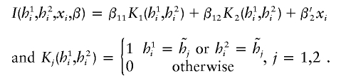
The associations of haplotypes of multiple SNPs and other covariates with the disease phenotype are quantified through the penetrance function (i.e., penetrance of haplotypes and other covariates to the disease phenotype). To model this penetrance function, we consider a logistic regression that relates haplotypes and covariates with the disease phenotype. Now let I(h1i,h2i,xi,β) denote a function of haplotypes (h1i,h2i), covariates (xi), and coefficients β. The logistic penetrance function can be formally defined as
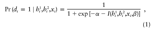 |
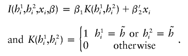
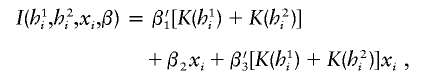
which takes values between 0 and 1, quantifying the probability of being affected. The function I(h1i,h2i,xi,β) is chosen according to the hypotheses of interest. For example, to assess the main associations of haplotypes and other covariates, one may choose
in which K(·) represents a vector of haplotype indicator functions. Depending on the context, the list of haplotypes may be fully specified, if they are chosen prior to the analysis, or may include all haplotypes observed in the data set. Haplotypes with high frequencies are termed “common haplotypes.” As in any typical categorical data analysis, it is desirable to use a common haplotype as the reference haplotype, unless a specific reference haplotype is preferred. “Rare” haplotypes (e.g., those observed with a frequency <5 within a given data set) may be collapsed into a composite haplotype for analytical purposes. Other choices for the function I(·) are listed below, in the “Analytic Strategies” subsection. The coefficient β in equation (1) can be estimated using the data collected from a case-control study design. Thus, the probability of being affected in a case-control study is
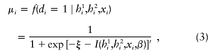 |
in which the intercept parameter ξ = α + log{[(1 − θ)η]/[θ(1 − η)]} represents a shifted intercept on the logit scale, θ is a fraction of cases in the study, and η is the probability of disease in the general population (Prentice and Pyke 1979). The rationale for choosing the logistic regression function is as follows: (i) regression coefficients (β1,β2) are readily interpretable as log odds ratios, and log odds ratios approximate log relative risk when disease incidence is low (Prentice and Mason 1986); (ii) the logistic regression technique has been well studied in biostatistical literature, and its statistical properties are well known; and (iii) logistic regression is routinely applied to epidemiological studies, to interpret results from case-control studies (Breslow and Day 1980), and is thus readily accepted in the study of gene-environment interactions. It is important to note that one regression coefficient is introduced for each common haplotype. If the number of common haplotypes becomes too large, then there may be too many parameters for estimation (see the “Discussion” section).
An Estimation Procedure
Conceptually, the analytic objective is to estimate parameters (ξ,β). If haplotypes were observable (e.g., in family studies or by experimental methods), one could construct an estimating function for (ξ,β) on the basis of the log likelihood function for logistic regression model (3). When unphased genotypes are observed in the studies, one can treat phases of genotypes as latent variables. After obtaining a posterior distribution of phase given all observed data (phenotypes, genotypes, and covariates), one can sum over all possible phases via the conditional expectation of the estimating function given the observed data. Setting the integrated estimating function to 0 results in equations for the estimation of (ξ,β). Derivation of estimating equations is detailed in appendix A.
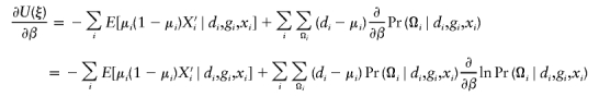
The estimates, denoted by  , satisfy the following estimating equations:
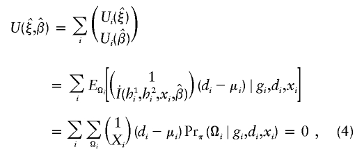 |
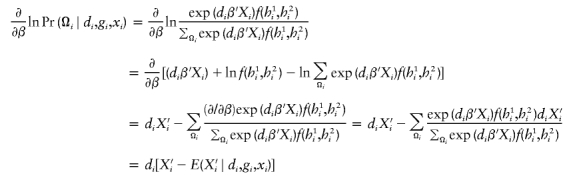
where the first summation is over all n independent samples, where  is the partial derivative of
  with respect to β, where
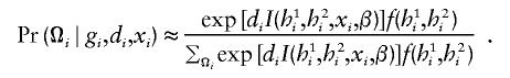
  is the posterior probability of the latent variables indexed by haplotype frequencies (π), Ωi, given the ith individual’s observed data, (gi,di,xi), and where π is a vector of the population frequencies of haplotypes. Under the rare-disease assumption, this conditional probability may be approximated to a simple formulation (see appendix B). Under Hardy-Weinberg equilibrium, the joint distribution of the paired haplotypes is equal to the product of the two marginal distributions—that is, fπ(h1i,h2i)=fπ(h1i)fπ(h2i). Hence, this conditional probability may be expressed as
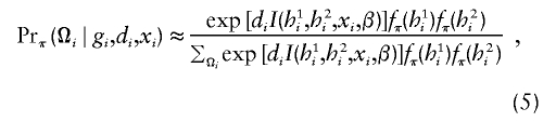 |
which is computable provided that the parameter β is known. Note that, for controls (di=0), the above posterior probability degenerates to a function of π through the joint distribution functions. Also note that the above conditional probability (eq. [5]) does not depend on the intercept ξ or α for either cases or controls, implying that the estimation would be robust regardless of this intercept.
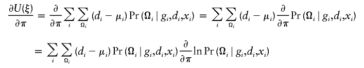
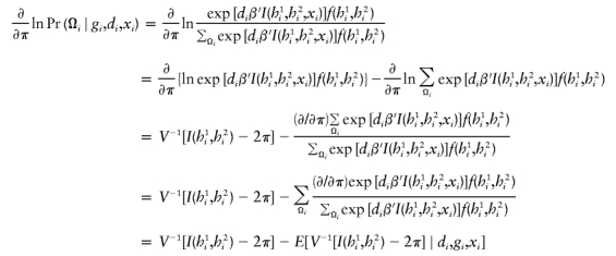
Under the rare-disease assumption, one can treat the control population as representative of the general population if it is a population-based case-control study (otherwise, one has to assume that selection of controls does not depend on SNPs and hence is unbiased) and estimate haplotype frequencies, π=(π1,π2,…,πH), for all possible haplotypes (h1,h2,…,hH), using only controls. To proceed with the estimation of haplotype frequencies in controls, we propose to use the following estimating equation, which has been derived elsewhere (Li et al., in press). Now let Fi=(Fi1,Fi2,…,FiH)′, in which Fij=I(h1i=hj)+I(h2i=hj)-2πj is the difference between the observed number and the expected number of the jth haplotype counts from the ith individual. Note that Fij—and, hence, Fi—is not specified unless phase Ωij is known. The equation for the estimation of haplotype frequencies may be written as
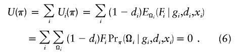 |
The estimate of π by use of estimating equation (6) is similar to that by the expectation-maximization algorithm (Excoffier and Slatkin 1995), except that the implementation based on equation (6) is more efficient and scalable to deal with a large number of SNPs.
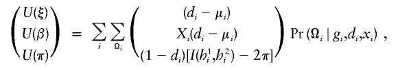
The estimates of (ξ,β,π), denoted as  , are jointly estimated using equations (4) and (6)—that is,
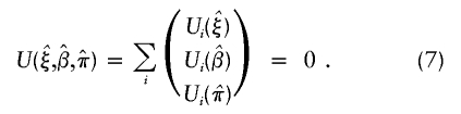 |
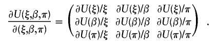
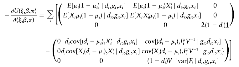
To proceed with the estimation, one needs to compute the derivative of U(ξ,β,π) with respect to all parameters (ξ,β,π) when using the Newton-Raphson method. As shown in appendix C, the derivative matrix of joint estimating equation (7), denoted as Γ(ξ,β,π), may be written as
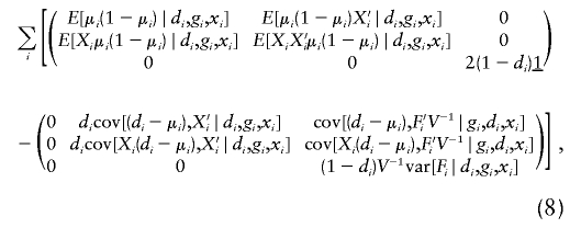 |
where 0 is a zero matrix of appropriate dimension. Conditional means, variances, and covariances are computed in the usual way in the above estimating equation.
Using the Newton-Raphson method, one can start from an initial value (ξ(0),β(0),π(0)) and iterate it to a new value (ξ(1),β(1),π(1)) via
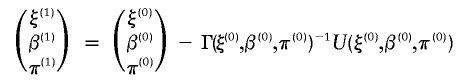 |
until convergence in all parameters is reached. Note that the burden of computing the conditional expectation over phase Ωi increases exponentially with the number of SNP loci. Thus, to ensure computational feasibility, our procedure approximates the expectation; for example,
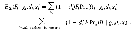 |
using only haplotypes with nontrivial haplotype frequencies. This procedure has been described elsewhere (Li et al., in press). Note that, in the framework of LOD-score methods (or likelihood), the estimating equation is the counterpart of the first derivative of the log likelihood (i.e., the score estimating equation), whereas the derivative of estimating function (i.e., the second derivative of the log likelihood function) is the counterpart of the information matrix.
Asymptotic Properties and Inferences
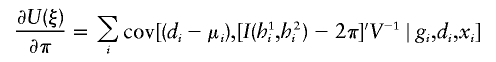
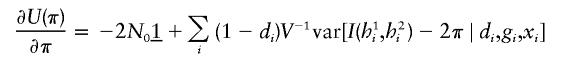
Joint estimating equation (7) is written as the summation of individual estimating functions over n independent samples. Applying the central-limit theorem (Godambe 1960; Liang and Zeger 1986), one can prove that, under the regularity conditions, the estimated parameters are consistent as n approaches infinity. Moreover, the estimated parameters have an asymptotic normal distribution with mean (ξ,β,π) and covariance Σ. One of the key regularity conditions is that the estimating functions in equation (7) approach 0 as the sample size increases (shown in appendix D). The covariance matrix, Σ, can be estimated by
where  is estimated by
  . This asymptotic distribution can now be used to construct either Wald-type or score-type statistics for inferences.
Analytic Strategies
The formulation of I(h1i,h2i,xi,β) in equation (1) can be modified to address various questions. Below, we list three formulations that may be useful as analytic strategies:
Haplotype-specific effects.—An immediate interest is to assess the disease associations with haplotypes. Earlier, we discussed the selection of haplotypes and let H denote the total number of those haplotypes. To assess their associations with the disease phenotype, one chooses equation (2) for I(h1i,h2i,xi,β), controlling for environmental covariates xi, and β1=(β11,…,β1H)′. Under the null hypothesis that the lth haplotype is not associated with the disease phenotype, the corresponding log odds ratio equals 0—that is, H0:β1l=0. To test this null hypothesis, one may use the Wald-type statistics for making inferences.
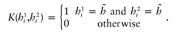
Diplotype-specific effects.—Although haplotype-based associations are of interest, the disease association could also be genotype specific; that is, the disease associates with genotypes at multiple loci formed by a pair of haplotypes, referred to as a “diplotype” (to differentiate it from a genotype formed by individual paired SNP alleles). Disease associations with a diplotype may be categorized by four different penetrance modes: dominant, recessive, additive, or codominant. To capture the mode of diplotype associations, one needs to recode corresponding diplotypes under each mode of penetrance. Suppose that  is the target haplotype of interest. Under a dominant mode, we would use the following indicator function:
 |
Similarly, if the recessive mode is considered, then one uses the same regression function but with
 |
Also, to model additive penetrance, one may choose the following indicator function:
Last, consider the codominant penetrance by two haplotypes  . The regression model is now written as
 |
The last model encompasses both dominant and additive modes as shown above. Specifically, if only one of the two coefficients (β11,β12) is not equal to 0, then the last model implies the dominant mode. If both coefficients (β11,β12) are ⩾0 and if the penetrance associated with both haplotypes  and
and  is the same, then the last model implies the additive mode.
Interactions between haplotypes and covariates.—The study of gene-environment interactions has long been of interest in genetic epidemiology (Khoury et al. 1993). In recent years, researchers in pharmacological research have been very interested in studying the interactions between drug treatment and genes. Additionally, researchers in clinical sciences have been interested in personalized medicine in the sense that physicians would like to prescribe treatments based on the patients’ genotypes. To model such gene-environment interactions, one would typically gather data on an array of covariates, including clinical, environmental factors or history of medications. We model the haplotype-covariate interaction via
 |
where the third term, β3=(β31,β32,…)′, quantifies the interactions of all candidate haplotypes with the single covariate. Indeed, one can postulate other models to depict interactions that may be dominant, recessive, or codominant, in addition to the additive mode described above.
Monte Carlo Simulation Studies
Recognizing that the inference methods above are based on asymptotic theories, we want to assess how well asymptotic results approximate distributions of the results with finite samples. Probably, the best way to evaluate the finite sample properties is via Monte Carlo simulation studies. The study population of haplotypes is simulated through a coalescent process. Simulation studies were conducted under both null hypotheses and alternative hypotheses. Using the simulations, we have also demonstrated possible confounding effects due to the admixture of subpopulations if the admixture is not adjusted in the model.
Simulating Data via the Coalescent Process
The simulation scheme generates a population of one million people, whose ages are randomly distributed from 20 to 80 years, with an equal number of men and women. We introduce a single candidate gene with 20 SNPs. The population distribution of all haplotypes is estimated on the basis of 2,000 haplotypes, generated by a simulation program of the coalescent process (obtained from R. Hudson’s Web site; see also Hudson 2002), in which one population is assumed, the number of segregation sites (i.e., SNPs) is specified as 20, the population recombination rate (R=4Ner, where Ne is the effective population size and r is the recombination rate) is specified as 0.4, and the number of sites between which the recombination can occur constitutes 1 kb. In the resulting population, 17 haplotypes were observed, with frequencies ranging from 0.23 to 0.001, estimated using 2,000 haplotypes (table 1). Individuals’ genotypes are generated by randomly drawing a pair of haplotypes from the distribution. We used the penetrance functions described in equations (1) and (2), set log odds ratio values, and then computed the expected disease probability. On the basis of the probability, we simulated the binary phenotype status by using a Bernoulli process. Treating the simulated one million individuals as the population, we generated a case-control sample by randomly selecting a subset of cases and controls with an equal number in each group. Analyzing the selected case-control sample data, we obtained estimates of the log odds ratios and their SEs for common haplotypes and covariates by using the method described above. For each specific set of coefficients, we repeated the simulation 1,000 times and summarized the simulation results of sample variations.
Table 1.
Distribution of Haplotypes[Note]
| Designation | Haplotype | Frequency |
| 0 | 00100000000000000000 | .2355 |
| 1 | 00000010000000000000 | .1825 |
| 2 | 00000100101100001000 | .1725 |
| 3 | 00000100101100000000 | .1170 |
| 4 | 01000100101100000000 | .1125 |
| 5 | 00001100101100001000 | .0970 |
| 6 | 00000011000000000000 | .0360 |
| 7 | 00000010000000010000 | .0170 |
| 8 | 00000010000000000001 | .0060 |
| 9 | 00000100101100000100 | .0055 |
| 10 | 01010100101100000000 | .0050 |
| 11 | 00000100101100001010 | .0045 |
| 12 | 00000010010000000000 | .0035 |
| 13 | 10000100101100001000 | .0030 |
| 14 | 00000100101110001000 | .0010 |
| 15 | 00001100101100101000 | .0010 |
| 16 | 00000010000001000000 | .0005 |
Note.— Estimated from 2,000 haplotypes created by use of Hudson’s (2002) simulation program of the coalescence process.
Statistical Measurements
We computed four customarily used measures to evaluate the performance of the proposed method in the estimation of log odds ratios  . From the jth replicate, let βj and
  represent the true and the estimate of the jth coefficient in equation (1), respectively. The first measure is the average bias in the estimation of β:
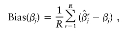 |
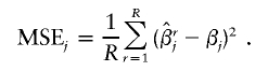
in which the summation is over all R replicates. In the current simulation study, we chose R=1,000. This quantity measures actual biases associated with each haplotype in the estimation of log odds ratios. The second measure is the accuracy of the estimate, quantified via the mean squared error (MSE), and is defined as
 |
Now, let  denote the estimated SE of
  for the rth replicate and let
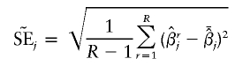 |
denote the estimate of the true SE of  . The third measure is the average bias in estimating the SE of
  :
:
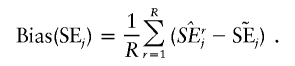 |
This measure quantifies the accuracy of the estimated SEs. The fourth measure is the coverage probability of the CI,  at the significance level of α (in this simulation study, α=0.05), that includes the true value βj. An acceptable coverage probability should approximate 1-α.
Simulation Studies under the Null Hypothesis
Under the assumption that none of haplotypes are associated with the disease, we set β11 = 0, β12 = 0, …, β1H in equation (1). For the remaining parameters in equation (1), we set α = −7, β21(sex) = 0, and β22(age − 20 years) = 0.05. In the current simulation, we chose the most frequent haplotype as the reference haplotype for all simulations. We performed simulation studies under the null hypothesis with varying sample sizes—100, 500, and 1,000—with equal numbers of cases and controls in each simulated data set. Results of the simulation are reported in table 2. Note that, as sample sizes vary, some haplotypes become rare in certain replicates and, hence, their corresponding coefficients are not computed individually, consequently causing missing estimates in some replicates. To avoid biases associated with such missingness, we choose to report estimates only if 600 of 1,000 simulation replicates yield estimated haplotype frequencies. Table 2 shows the four measures to evaluate the estimated coefficients, SEs, and coverage probabilities, for sample sizes of 100, 500, and 1,000. The first part of table 2 shows these measures for the covariates, which were sex and age. Clearly, all estimates are generally accurate and unbiased over the range of sample sizes, and, as the sample size increases, the coverage probabilities approach 0.95, the desired level. The second part of table 2 shows the four measures evaluated for the estimated haplotype-related parameters. In all, 10 common haplotypes are included, with respective frequencies ranging from 0.006 to 0.235 (the most common haplotype is treated as the reference haplotype). Under the null hypothesis, none of haplotypes are associated with the disease phenotype, and, hence, corresponding regression coefficients equal 0, as noted in table 2 (under “True βj”). Also note that, when the sample size is small, many less common haplotypes have estimated haplotype frequencies below some threshold (e.g., expected number of haplotypes should be greater than or equal to five) and hence are not included in the list of selected haplotypes, resulting in fewer haplotypes. For example, 4 of the 10 haplotypes are absent in the empirical data with a sample size of 100, and 2 are absent with a sample size of 500; but all 10 are present when the sample size increases to 1,000. Regardless of sample size and frequencies of haplotypes, biases in the estimated regression coefficients and SEs are small. Accuracy, quantified by MSEs, steadily improves with increasing sample sizes. Correspondingly, coverage probabilities are generally ∼0.95, showing that statistical inference maintains its appropriate type I error rate.
Table 2.
Simulation Results for the Model under the Null Hypothesis[Note]
| 50 × 2a |
250 × 2a |
500 × 2a |
||||||||||||
| Covariate | Mean | True βj | Bias(βj) | MSE(βj) | Bias(SEj) | 95% Coverage Probability | Bias(βj) | MSE(βj) | Bias(SEj) | 95% Coverage Probability | Bias(βj) | MSE(βj) | Bias(SEj) | 95% Coverage Probability |
| Sex | 50% male | 0 | .013 | .237 | −.006 | .962 | .014 | .037 | .006 | .949 | .007 | .019 | .003 | .955 |
| Age | 50 years | .05 | .006 | .000 | −.002 | .938 | .002 | .000 | −.000 | .951 | .001 | .000 | −.000 | .954 |
| 50 × 2a |
250 × 2a |
500 × 2a |
||||||||||||
| Haplotype | Frequency | True βj | Bias(βj) | MSE(βj) | Bias(SEj) | 95% Coverage Probability | Bias(βj) | MSE(βj) | Bias(SEj) | 95% Coverage Probability | Bias(βj) | MSE(βj) | Bias(SEj) | 95% Coverage Probability |
| 0 | .235 | …b | ||||||||||||
| 1 | .183 | 0 | .043 | .274 | −.022 | .942 | −.007 | .043 | .003 | .955 | −.022 | .024 | −.004 | .944 |
| 2 | .173 | 0 | .058 | .321 | −.045 | .930 | −.023 | .051 | −.006 | .942 | −.041 | .026 | −.000 | .942 |
| 3 | .117 | 0 | .085 | .408 | −.044 | .946 | −.032 | .065 | −.003 | .948 | −.050 | .031 | .007 | .947 |
| 4 | .113 | 0 | .066 | .443 | −.060 | .939 | −.024 | .063 | .002 | .953 | −.068 | .035 | .002 | .938 |
| 5 | .097 | 0 | .108 | .435 | −.028 | .941 | .005 | .067 | .001 | .957 | −.014 | .033 | .001 | .955 |
| 6 | .036 | 0 | −.080 | .165 | .002 | .959 | −.097 | .087 | −.001 | .934 | ||||
| 7 | .017 | 0 | −.011 | .385 | −.047 | .947 | −.028 | .174 | −.009 | .958 | ||||
| 8 | .006 | 0 | .194 | .369 | −.019 | .955 | ||||||||
| 9 | .006 | 0 | .111 | .320 | −.043 | .956 | ||||||||
Note.— None of 16 haplotypes are associated with the disease. Summary statistics are reported only for the haplotypes that have been considered as common haplotypes, and their associated coefficients have been estimated in >600 of 1,000 simulations.
Sample sizes of cases and controls.
Reference.
Simulation Studies under the Alternative Hypothesis
We assumed that two haplotypes, the third and the eighth, were associated with the disease, with log odds ratios of −1 and 5, respectively. A negative log odds ratio (e.g., −1) indicates that an individual carrying that haplotype has a reduced disease risk, 0.37 times less than that of an individual carrying the most common haplotype. Similarly, a positive log odds ratio (e.g., 5) indicates an increased risk, 148 times more than that of an individual carrying the most frequent haplotype. As might be expected, the frequency of such a high-risk haplotype needs to be quite low (0.017), without causing an epidemic in the simulated population.
Table 3 shows the bias measures and coverage probabilities in the same format as in table 2. Whereas two haplotypes are shown to associate with the disease phenotype, estimated regression coefficients and their SEs for both covariates center around the true values, and biases decrease as sample sizes increase. Accuracy measurements for some haplotypes are rather poor when the sample size is small but are improved enormously when the sample size increases to 500. Coverage probabilities are smaller than the expected 0.95 when the sample size is 100 but gradually approach 0.95 as the sample sizes increase to 500 and 1,000. The second part of table 3 shows biases associated with the haplotypes. Biases are minor, and coverage probabilities are generally ∼0.95. Of particular interest are the two haplotypes associated with the disease phenotype. For the third haplotype (2 in table 3), biases in the estimation of the log odds ratio steadily decrease with increasing sample size, and biases in the estimation of SEs drop significantly when the sample size increases from 100 to 500. Again, coverage probabilities approach 0.95 as the sample size increases. Regarding the high-risk haplotype (7 in table 3), the biases in the estimation of log odds ratios and their SEs gradually decrease as the sample size increases. Interestingly, the coverage probabilities are ⩾0.95 at all sample sizes. Note that rare haplotypes are not included in some of simulation replicates, and their coefficients are thus not estimated, resulting in truncation effects. It appears that the truncation effects of the selection of completely estimated haplotypes might have a modest impact on coverage probabilities.
Table 3.
Simulation Results for the Model under the Alternative Hypothesis[Note]
| 50 × 2a |
250 × 2a |
500 × 2a |
||||||||||||
| Covariate | Mean | True βj | Bias(βj) | MSE(βj) | Bias(SEj) | 95% Coverage Probability | Bias(βj) | MSE(βj) | Bias(SEj) | 95% Coverage Probability | Bias(βj) | MSE(βj) | Bias(SEj) | 95% Coverage Probability |
| Sex | 50% male | 0 | .021 | .962 | −.127 | .936 | .024 | .097 | −.013 | .940 | .016 | .043 | −.002 | .950 |
| Age | 50 years | .05 | .016 | .002 | −.009 | .928 | .003 | .000 | −.000 | .950 | .002 | .000 | .000 | .946 |
| 50 × 2a |
250 × 2a |
500 × 2a |
||||||||||||
| Haplotype | Frequency | True βj | Bias(βj) | MSE(βj) | Bias(SEj) | 95% Coverage Probability | Bias(βj) | MSE(βj) | Bias(SEj) | 95% Coverage Probability | Bias(βj) | MSE(βj) | Bias(SEj) | 95% Coverage Probability |
| 0 | .235 | …b | ||||||||||||
| 1 | .183 | 0 | .102 | 1.001 | −.157 | .924 | .008 | .092 | .003 | .955 | .003 | .043 | .006 | .960 |
| 2 | .173 | −1 | −.112 | 3.037 | −.626 | .913 | −.098 | .179 | −.002 | .948 | −.066 | .081 | .006 | .955 |
| 3 | .117 | 0 | .046 | 1.916 | −.344 | .920 | −.046 | .139 | −.009 | .949 | −.053 | .070 | −.008 | .947 |
| 4 | .113 | 0 | .086 | 1.246 | −.168 | .920 | −.072 | .137 | .001 | .950 | −.084 | .070 | .003 | .947 |
| 5 | .097 | 0 | .122 | 1.416 | −.219 | .931 | −.040 | .166 | −.024 | .939 | −.031 | .075 | −.007 | .949 |
| 6 | .036 | 0 | −.063 | .377 | −.036 | .945 | −.083 | .175 | −.011 | .943 | ||||
| 7 | .017 | 5 | .924 | 6.181 | −1.63 | .950c | .195 | .323 | .001 | .967 | .066 | .140 | .004 | .968 |
| 8 | .006 | 0 | .063 | .440 | −.103 | .888c | ||||||||
| 9 | .006 | 0 | .139 | .299 | −.112 | .896c | ||||||||
Note.— The third and eighth haplotypes are associated with the disease. Summary statistics are given for the haplotypes reported in table 1 and for the disease-associated haplotype.
Sample sizes of cases and controls.
Reference.
The haplotype's associated coefficient has been estimated in <600 of 1,000 simulations, because these haplotypes are rare in some simulations and hence their coefficients are not estimated, resulting in truncation effects.
Simulation Studies in the Presence of Population Admixture
One concern with the direct assessment of genetic association with disease phenotype in case-control studies is the admixture of populations, without appropriate accounting for population origin. Admixture of populations occurs when an allele is associated with the population origin and when different populations have different levels of risks. In epidemiology literature, the admixture of populations is considered a potential confounding factor because of its association with both genetic factors and disease phenotype (Rothman and Greenland 1998). An effective way of controlling for such confounding effects is to identify them and then to adjust for them in the regression analysis. To illustrate the phenomenon of admixture, we performed the following simulation: Consider a population with an admixture of two racial groups, 70% of European origin and 30% of African American origin (proportions similar to those found in a recent multicenter study of breast cancer; see Britton et al. 2002). Also assume that, in comparison with an individual of European origin, an individual of African American origin has twice the risk of disease. Suppose that haplotype distributions of these two populations are different. Hence, by definition, the population origin may be a confounding factor. In this simulation, none of the haplotypes were associated with the disease phenotype. Using the coalescent process described above, we generate haplotype frequencies among whites. These are given in the second part of table 4 (under “Frequency among Whites”). For African Americans, we assumed that the second and third haplotypes were absent, emulating the phenomenon that certain haplotypes are prevalent among whites but are nearly absent in people of African origin. Frequencies for the remaining haplotypes among African American are normalized to add up to 1. Under these assumptions, the simulation creates a mixture of two subpopulations. We chose a sample size of 500, with 250 cases and 250 controls.
Table 4.
Simulation Results for the Model with Admixture Population[Note]
|
With Adjustment for Race |
Without Adjustment for Race |
||||||||||
| Covariate | Mean | True βj | Bias(βj) | MSE(βj) | Bias(SEj) | 95% Coverage Probability | Bias(βj) | MSE(βj) | Bias(SEj) | 95% Coverage Probability | |
| Sex | 50% male | 0 | −.008 | .052 | .006 | .954 | .000 | .045 | .025 | .951 | |
| Age | 50 years | .05 | .001 | .000 | .002 | .961 | .000 | .000 | .003 | .961 | |
| Race | 30% black | 2 | .014 | .080 | .038 | .924 | |||||
|
Frequency among |
With Adjustment for Race |
Without Adjustment for Race |
|||||||||
| Haplotype | Whites | Blacks | True βj | Bias(βj) | MSE(βj) | Bias(SEj) | 95% Coverage Probability | Bias(βj) | MSE(βj) | Bias(SEj) | 95% Coverage Probability |
| 0 | .235 | .382 | …a | ||||||||
| 1 | .183 | 0 | 0 | −.020 | .111 | .001 | .942 | −1.10 | 1.311 | −.021 | .045 |
| 2 | .173 | 0 | 0 | .037 | .106 | .011 | .960 | −1.02 | 1.142 | .002 | .055 |
| 3 | .117 | .190 | 0 | .063 | .066 | −.005 | .942 | .051 | .053 | −.002 | .946 |
| 4 | .113 | .184 | 0 | .063 | .067 | −.006 | .938 | .058 | .057 | −.005 | .942 |
| 5 | .097 | .158 | 0 | .018 | .070 | −.007 | .945 | .015 | .057 | −.002 | .952 |
| 6 | .036 | .059 | 0 | .091 | .166 | −.011 | .943 | .073 | .135 | −.008 | .934 |
| 7 | .017 | .028 | 0 | .130 | .369 | −.031 | .940 | .093 | .306 | −.027 | .952 |
Note.— For 250 cases and 250 controls.
Reference.
Table 4 gives the bias measures and the coverage probabilities from simulation studies in the presence of population admixture. We have done two separate analyses: with and without adjustment for the race covariate. The results when the race covariate is included in the logistic regression model are presented under the heading “With Adjustment for Race.” All estimated regression coefficients and their SEs, for covariates and haplotypes, appear to be unbiased and accurate, and their coverage probabilities are generally ∼0.95. The results when the race covariate is not included (i.e., without adjustment for population admixture) are presented under the heading “Without Adjustment for Race.” Interestingly, estimated regression coefficients for sex and age, two covariates in the first two models, are unbiased and accurate, as are the estimates of their SEs, and coverage probabilities are also ∼0.95, demonstrating that associations with sex and age can be correctly assessed. However, estimated regression coefficients for haplotypes 1 and 2 are substantially biased (by as much as −1), accuracy of estimates is rather poor, and the coverage probabilities are grossly underestimated. Estimated SEs do not have any significant biases, implying that the distribution of these biased estimates resembles that of unbiased estimates. For the remaining haplotypes, estimated regression coefficients and their standard appear to be unbiased, accuracy is acceptable, and estimated coverage probabilities are ∼0.95. Indeed, this result demonstrates how much population admixture could affect estimated haplotype-associations and demonstrates that such biases could be virtually eliminated, once the confounding factor is controlled via the regression models.
A Case-Control Study with Six SNPs of Apolipoprotein CIII
The study and its sampling process have been described in detail elsewhere (Cheng et al. 1999; Zee et al 2002). In brief, within a cohort of 779 patients undergoing percutaneous transluminal coronary angioplasty, 342 developed restenosis within 6 mo (case patients), whereas 437 remained restenosis free (control individuals). From each participant, blood samples were collected and were genotyped for SNPs in seven candidate genes, including apolipoprotein CIII. Six SNPs (C−628A, C−482T, T−455C, C1100T, C3175G, and T3206G) in the apolipoprotein CIII gene were genotyped. The objective of this analysis was to discover haplotypes, of these six SNPs, that were significantly associated with the disease phenotype. We analyzed the genotype data at individual loci by using the logistic regression model described in the “Methods” section, and we estimated haplotype frequencies and their SEs, as well as odds ratios and their 95% CIs. The analysis identified 11 common haplotypes, shown in table 5. Two haplotype sequences (CCTTCG and ACCCCT) have odds ratios of 0.63 and 0.61 and 95% CIs of 0.44–0.91 and 0.38–0.97, respectively. This result suggests that individuals with haplotype CCTTCG or haplotype ACCCCT are likely to be at a significantly lower risk for the disease, in comparison with those with most common haplotype sequence (CCTCCT). Even though the haplotype-based association is modest, this finding is interesting in the context of earlier analyses performed by Zee et al. (2002), who have shown that, by univariate analyses, none of individual SNP alleles in apolipoprotein CIII are significantly associated with restenosis. However, in the multiple logistic regression analysis that includes multiple SNPs, apolipoprotein CIII was identified as one of most significant predictors for the occurrence of restenosis.
Table 5.
Estimated Haplotype Frequencies and Their SEs for All Common Haplotypes[Note]
| SNP Marker (Sequence) | HaplotypeFrequency | SE | Odds Ratio (95% CI) |
| 000000 (CCTCCT) | .401 | .017 | 1.00 (reference) |
| 111000 (ATCCCT) | .118 | .012 | 1.01 (.70–1.45) |
| 000101 (CCTTCG) | .128 | .013 | .63a (.44–.91) |
| 111111 (ATCTGG) | .077 | .009 | 1.02 (.70–1.51) |
| 101000 (ACCCCT) | .082 | .010 | .61a (.38–.97) |
| 000001 (CCTCCG) | .065 | .010 | 1.16 (.73–1.86) |
| 111101 (ATCTCG) | .047 | .010 | .73 (.41–1.31) |
| 101001 (ACCCCG) | .029 | .007 | .96 (.49–1.86) |
| 111001 (ATCCCG) | .017 | .012 | .55 (.14–2.16) |
| 110101 (ATTTCG) | .013 | .004 | .93 (.38–2.29) |
| 000100 (CCTTCT) | .009 | .004 | .90 (.29–2.82) |
Note.— Expected number of each haplotypes is ⩾5 copies.
Indicates that the odds ratio is different from one at a significance level of 5%.
Discussion
We have introduced an estimating-equation approach for the assessment of disease associations with SNP haplotypes when adjustment for covariates (e.g., environmental factors, lifestyle variables, clinical variables, or treatment) is performed in case-control studies. This method has several notable properties: First, it is designed for case-control studies with no available family data. If family data were available, it could be used to improve haplotyping efficiency. Second, this method focuses on associations between haplotype distributions and the disease phenotype, thus avoiding misclassification errors due to the “reconstructions of haplotypes.” Third, this method can be scaled up to deal with >100 SNPs. Fourth, it does not require any assumptions of linkage disequilibrium, recombination, or other population genetic parameters, and, hence, the results tend to be robust. Of course, in the presence of strong linkage disequilibrium, the current method becomes particularly efficient in identifying common haplotypes and further estimating their haplotype frequencies. The analytic derivation helps us to prove that estimated regression coefficients are consistent and that they have asymptotic normal distributions with appropriately estimated asymptotic variances. To evaluate approximations of asymptotic results in finite samples, we performed Monte Carlo simulations. Simulation results demonstrated that estimated regression coefficients in the logistic regression are generally unbiased and that estimated SEs are correct. Finally, coverage probabilities are close to the desired level, so that the false-positive error rates are controlled.
Also using the Monte Carlo simulation method, we assessed the impact that admixture had on estimated regression coefficients, SEs, and coverage probabilities. When adjustment for the population origin is not made in the logistic regression model, simulation results show that estimated regression coefficients for the “confounding haplotypes” are clearly biased, consistent with the concern regarding admixture (Elston 1999). The simulation results also show that biases due to admixture could be minimized, if the associated sources are identified and incorporated into the logistic regression model.
The challenge in correction for admixture biases is that the population origin is often unknown. For example, within the same racial group—such as whites from different parts of Europe—individuals may have different genetic constellations, owing to differences in their recent evolutionary history. One approach is to use a latent-class model to account for unmeasured population substructures (Satten et al. 2001), but its validity relies on assumptions about latent-class models. An alternative approach is to gather a set of genetic markers that are known to vary from ethnic group to ethnic group and to perform cluster analysis on subjects of identified subpopulations (Pritchard et al. 2000). Once subpopulations are discovered, the population structure can then be adjusted for, using the methods described in the present article. When ethnicity-related genetic markers are gathered, one can also treat them as surrogates and simply adjust for them via the logistic regression model described above.
Although we appreciate the strengths of this methodology, it is also important to discuss its potential limitations. First, when the number of common haplotypes is relatively large, the procedure may involve estimation of many regression coefficients in the logistic regression (eq. [1]). As in typical categorical data analyses, estimating an excessive number of parameters diminishes the power of such analysis. To avoid this limitation, one needs to focus on situations in which the number of common haplotypes is relatively small; for example, when multiple SNPs arise from a single candidate gene or when 10–100 physically adjacent SNPs are considered, the number of common haplotypes has been shown to be much fewer than the theoretical number of all possible haplotypes (Drysdale et al. 2000; Daly et al. 2001). In the event that the analysis has to deal with many common haplotypes, it is advisable to adopt a stepwise procedure: evaluating common haplotypes one at a time by the regression model, then two at a time, and promptly terminating the stepwise procedure when the regression model is saturated. Another limitation of this method is associated with the rare-disease assumption. Under this assumption, haplotype frequencies computed on the basis of controls approximate those in the general population. Specifically, a population haplotype frequency may be decomposed into the weighted average of haplotype frequencies in controls and in cases, via π = π0Pr(d=0)+π1Pr(d=1). The bias in the estimation of haplotype frequency by use of controls may be written as π-π0=-π0[1-Pr(d=0)]+π1Pr(d=1)=Pr(d=1)(π1-π0). Because π1 and π2 are between 0 and 1 and, hence, (π1-π0) ranges from −1 to 1, the absolute value of this bias is less than Pr(d=1). When the disease incidence rate is <1%, the bias in the estimation of haplotype frequencies is <1%. However, if this analytic approach is used for common traits (e.g., a certain hair color), then this bias could be substantial. Of course, when dealing with common traits, one probably would not choose a case-control design. The third limitation worth noting is that the assumptions of the logistic regression model itself (eq. [1]) could be violated. For example, the probability of being affected may be linearly associated with haplotypes and/or covariates, or the functional relationship may follow an exponential form. Nevertheless, one can always view the logistic regression as an empirical model, approximating the relationship of the disease probability with haplotypes and covariates. In fact, in the absence of covariates, the logistic form imposes no assumptions.
As noted earlier (in the “Introduction” section), other methods may also be used for the analysis of multiple SNPs in case-control studies. One method is to correlate individual SNP genotypes (0/0, 0/1, and 1/1) or their combinations with the disease phenotype by using, for example, logistic regression (Breslow and Day 1980). An example of such an approach is the stepwise strategy for the selection of SNP alleles—or logical combinations of SNP alleles—with the strongest statistical associations, as has been explored by Cordell and Clayton (2002). Although conceptually straightforward, this method may become inefficient, since it has to numerate through all possible combinations of SNPs without taking advantage of the preserved haplotype structure within a functional gene. Furthermore, the interpretation of regression coefficients associated with genotypes at multiple loci and their cross products is also challenging. In contrast, our method uses the genomic structure to construct the distribution of common haplotypes. Since the number of common haplotypes in the population is small, our approach effectively reduces the large dimensionality of all possible haplotypes to a few and is thus an effective and meaningful way to gain statistical efficiency in the discovery of haplotypes of interest. However, if multiple SNPs were selected randomly from the genome, the number of common haplotypes is expected to be high. In this case, the advantage of our approach is diminished. Hence, haplotype-based methods, such as the one proposed in the present article, should be used either for multiple SNPs within candidate genes or when selected SNPs are physically close to each other.
Indeed, our haplotype-based method is closely connected with several other haplotype-based methods that correlate multiple SNPs with complex disease phenotypes (Hartl and Clark 1997; Drysdale et al. 2000). One such method in family studies is to collect genotype data from both parents and to compare individual marker alleles with the father’s and mother’s alleles, to determine the phase of alleles (Wijsman 1987). Although family-based haplotyping is thought to be ideal, routine gathering of genotypes from parents in case-control studies is costly and ethically sensitive. Hence, the family-based case-control study may be challenging unless such family data have already been gathered and genotypes are readily available. Alternatively, one may haplotype multiple SNPs experimentally (Weston et al. 1992)—for example, using long-range PCR or in vitro hybridization (Vogelstein and Kinzler 1998; Fallin and Schork 2000). However, experimental phase-resolution methods remain impractical for large numbers of SNPs and are not upwardly scalable to a large number of SNPs.
Another class of haplotype-based methods, one that does not rely on experimental methods or on family data, is to statistically infer haplotypes from multiple SNPs. The cladistic method is applicable to haplotype-based analysis with three or four SNPs. Basically, from all cases and controls, one can unambiguously identify haplotypes of several SNPs, on a subset of cases and a subset of controls, and use these identified haplotypes to establish the correlation of interest, ignoring the remaining haplotypes (Haviland et al. 1995). As expected, ignoring partially informative haplotypes leads to a loss of efficiency, which can become quite significant as the number of SNPs increases. Typically, such a method is applicable to, at most, three or four SNPs. Recently, Schaid et al. (2002) have proposed a score test for haplotype association. Because the test statistic is generated under the null hypothesis, it requires calculation of haplotype-related distribution for the entire population, without inferring haplotypes for individual subjects, thus bypassing the computational challenge described here. However, the key assumption required by the test statistics is the absence of gene-environment interaction. Additionally, one is unable to estimate haplotype-specific log odds ratios, which could be useful for further validation studies, as well as for genetic counseling. For the reconstruction of haplotypes by use of partially observed phase information, another class of methods is to infer haplotypes on the basis of empirical distributions, tolerating some degree of misclassification error (Hallman et al. 1999). Recently, a Markov-chain Monte Carlo method to estimate haplotype frequencies, as well as to construct haplotypes, has been proposed (Stephens et al. 2001). Likewise, Niu et al. (2002) have proposed a Bayesian method to estimate haplotype frequencies, as well as to infer haplotypes. However, reconstructed haplotypes, regardless of analytic strategies, will experience a degree of misclassification error. If such errors are naively ignored in the downstream analysis, then they may bias estimated parameters and inflate false-positive errors.
To demonstrate this point, we considered two possible analyses with reconstructed haplotypes via a logistic regression. One analysis uses the best-reconstructed haplotypes as covariates in the logistic regression analysis, whereas the other includes the best-reconstructed haplotypes only if their calculated probabilities are >80%. Using the coalescent process described above, we simulated several different data sets and applied the two logistic regression analyses along with our method. Interestingly, we found that in several simulations, in which haplotypes can be reliably inferred, results from all three analyses are fairly comparable (not shown). Furthermore, under the null hypothesis, estimates appear to be unbiased and to retain appropriate coverage probabilities. In contrast, when haplotypes cannot be reliably inferred and certain haplotypes are significantly associated with the phenotype, biases inherent in the reconstruction of haplotypes could be rather significant, an example of which is shown in table 6. Clearly, both logistic regression analyses have substantial biases, and their coverage probabilities are not consistent with the designated 95%. Systematic comparison of methods using reconstructed haplotypes versus our methods is very important, and a full exploration of this comparison is beyond the scope of the present article. A separate article will report findings from a systematic comparison.
Table 6.
Simulation Results for Comparisons between HPlus and Two Logistic Regression Analyses with Reconstructed Haplotypes
|
Proposed Method |
First Logistic Regression Methoda |
Second Logistic Regression Methodb |
||||||||||||
| Covariate | Mean | True βj | Bias(βj) | MSE(βj) | Bias(SEj) | 95% Coverage Probability | Bias(βj) | MSE(βj) | Bias(SEj) | 95% Coverage Probability | Bias(βj) | MSE(βj) | Bias(SEj) | 95% Coverage Probability |
| Sex | 50% male | 0 | .009 | .031 | .003 | .956 | .007 | .029 | .004 | .954 | .017 | .041 | −.002 | .951 |
| Age | 50 years | .05 | .001 | .000 | −.000 | .940 | −.000 | .000 | −.000 | .938 | .001 | .000 | −000 | .928 |
|
Proposed Method |
First Logistic Regression Methoda |
Second Logistic Regression Methodb |
||||||||||||
| Haplotype | Frequency | True βj | Bias(βj) | MSE(βj) | Bias(SEj) | 95% Coverage Probability | Bias(βj) | MSE(βj) | Bias(SEj) | 95% Coverage Probability | Bias(βj) | MSE(βj) | Bias(SEj) | 95% Coverage Probability |
| 0 | .159 | …c | ||||||||||||
| 1 | .140 | 0 | −.020 | .058 | −.017 | .933 | −.240 | .110 | −.003 | .829 | −.127 | .101 | −.005 | .933 |
| 2 | .108 | 0 | −.015 | .072 | −.012 | .949 | −.067 | .073 | −.039 | .890 | .011 | .074 | −.019 | .937 |
| 3 | .107 | 3 | −.018 | .047 | −.018 | .928 | −.368 | .167 | .010 | .498 | −.084 | .059 | −.003 | .928 |
| 4 | .095 | 0 | −.050 | .079 | −.011 | .939 | −.200 | .115 | −.029 | .840 | −.044 | .076 | −.001 | .937 |
| 5 | .076 | 0 | .016 | .097 | .001 | .953 | .543 | .458 | −.149 | .474 | .120 | .117 | −.021 | .905 |
| 6 | .060 | 0 | −.030 | .109 | −.009 | .946 | −.233 | .155 | −.015 | .878 | −.082 | .115 | −.006 | .942 |
| 7 | .044 | 0 | −.018 | .150 | −.026 | .935 | −.283 | .232 | −.026 | .847 | −.098 | .236 | −.036 | .935 |
Uses the best-reconstructed haplotypes.
Uses the best-reconstructed haplotypes with the reconstruction probability >80%.
Reference.
We are encouraged by the preliminary results obtained to date, and we plan several further improvements. First, we plan to perform more simulation studies, under various plausible scenarios, such as different haplotype-frequency patterns, different degrees of recombination, and different degrees of association. Second, it is also important to compare this approach with the current standard approach, which treats inferred haplotypes as true haplotypes in the logistic regression. Although, theoretically, the standard approaches could induce biases, a more practical issue is, What is the magnitude of the biases with practical sample sizes? Third, a natural extension of the current approach would be to incorporate nonbinary phenotypes, such as continuous phenotypes. Finally, we intend to develop methods for the evaluation of case-control study designs, such as the number of cases and controls required to achieve the desired power.
A compiled computer program, HPlus, has been developed. It is available to academic researchers on request, for use in not-for-profit research.
In summary, the completion of the Human Genome Project will provide an array of SNPs from 30,000–40,000 functional genes (International Human Genome Sequencing Consortium 2001; Venter et al. 2001). The availability of these SNPs will allow us to directly assess their associations with phenotypes of interest, regardless of whether such phenotypes have any obvious familial tendency. Equipped with appropriate study designs and analytic tools, investigators will be able to conduct population-based genetic studies focusing on associations of both genes and environmental factors with complex diseases.
Acknowledgments
We would like to thank Antonio Fernandez-Ortiz, Carlos Macaya, Emilio Pintor, and Arturo Fernandez-Cruz, from the Hospital Universitario San Carlos, Ciudad Universitaria (Madrid); Suzanne Cheng and Michael Grow, from Roche Molecular Systems (Alameda, CA); Robert Y. L. Zee, from the Department of Medicine at Brigham and Women’s Hospital (Boston); and Klaus Lindpaintner, from Roche Genetics, F. Hoffmann–La Roche (Basel, Switzerland). In addition, we thank the Max Delbruck Centre for Molecular Medicine (Berlin) and F. Hoffmann–La Roche (Basel, Switzerland), for their effort in the collection of patient data and the genotyping of SNPs. We would also like to acknowledge Suzanne Cheng and Christopher Carlson, for their earlier involvement in developing this project, and Klaus Lindpaintner, for his helpful comments on the resulting interpretation. Finally, we would like to thank the reviewers, whose comments and suggestions have greatly enhanced the presentation of this work. This work was supported, in part, by grants from the National Institutes of Health.
Appendix A: Derivation of the Estimating Equations
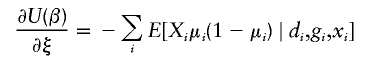
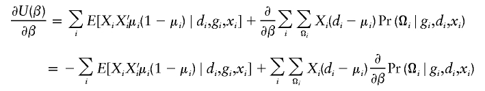
There is a wealth of literature on logistic regression and its variations for case-control studies (Cox 1972; Prentice and Pyke 1979). On the basis of the retrospective log likelihood function, one can readily formulate the estimating equation for (ξ,β) as
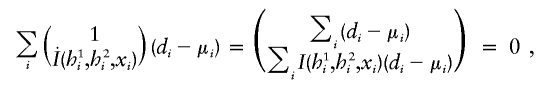 |
where  is the partial derivative of
  and (di,μi) are the disease phenotype and the mean as defined in equation (3). Note that the first equality of 0 ensures the constraint associated with case-control studies (Whittemore 1995).
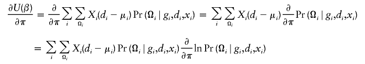
When phases Ωi are unknown, one may construct an estimating equation by integrating latent phases, and the resulting estimating equation U(ξ,β) may be written as
 |
where the conditional expectation is defined through the conditional probability f(Ωi∣gi,di,xi). The conditional probability, which can be approximated, is derived in appendix B.
Appendix B: Approximation to f(Ωi∣gi,di,xi)
By Bayes’ rule, the probability function may be written as
 |
under the assumption that the covariates are independent of haplotypes. When the disease phenotype is uncommon, the marginal probability of disease Pr(di=1∣h1i,h2i,xi) is small, and the marginal probability of nondisease Pr(di=0∣h1i,h2i,xi) is close to 1. Hence, the disease probability may be approximated by
 |
since exp[α+I(h1i,h2i,xi,β)] is much smaller than 1. Substituting these approximations into the above probability function, one obtains, for cases, an approximated function,
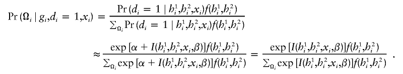 |
Similarly, for controls, the approximation is
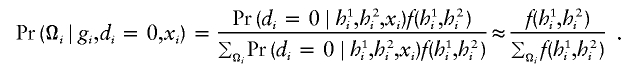 |
Putting these together, Pr(Ωi∣gi,di,xi) may be represented by
 |
Appendix C: Derivation of Derivative Matrix for the Joint Estimating Equation
As noted in the text, the joint estimating equation for (ξ,β,π) may be written as
 |
where  represents a vector of covariate function; the indicator function I(h1i,h2i) is used here generically to denote
  . Note that, by construction, Xi should be free from any unknown parameters. The derivative matrix of the above joint estimating equation with respect to (ξ,β,π) may be written as
 |
Let the notation (i,j) denote the ith row and the jth column in the above derivative matrix. All elements in the above derivative matrix are listed below:
-
(1,1)

-
(1,2)

-
(1,3)
-
(2,1)
-
(2,2)

-
(2,3)
-
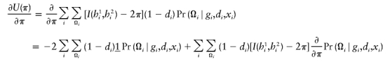
(3,1)
-
(3,2)
-
(3,3)
in which Fi=I(h1i,h2i)-2π.
Appendix D: Consistency of Estimates of (ξ,β)
One important aspect of this development is to prove the consistency of estimating equations, in the sense that estimated parameters are consistent as the number of samples approaches ∞. To prove this consistency, it is sufficient to prove that the estimating function asymptotically approaches 0. Consider the situation in which haplotype frequencies are consistently estimated and are held consistent. By the law of large numbers, the estimating function on the left-hand side of equation (4), divided by the sample size n, may be approximated by
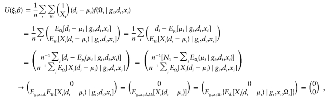 |
where n1 is the number of cases and “→” represents convergence, when the number of independent samples becomes sufficiently large. Hence, the estimating function above approaches 0 asymptotically. This convergence indicates that estimated parameter is also consistent via the Taylor expansion.
Electronic-Database Information
The URL for data presented herein is as follows:
- R. Hudson’s Web Site, http://home.uchicago.edu/~rhudson1/source/mksamples.html
References
- Breslow NE, Day NE (1980) Statistical methods in cancer research. International Agency for Research on Cancer, Lyon, France [Google Scholar]
- Britton JA, Gammon MD, Schoenberg JB, Stanford JL, Coates RJ, Swanson CA, Potischman N, Malone KE, Brogan DJ, Daling JR, Brinton LA (2002) Risk of breast cancer classified by joint estrogen receptor and progesterone receptor status among women 20–44 years of age. Am J Epidemiol 156:507–516 [DOI] [PubMed] [Google Scholar]
- Chakravarti A (1998) It’s raining SNPs, hallelujah? Nat Genet 19:216–217 [DOI] [PubMed] [Google Scholar]
- ——— (1999) Population genetics—making sense out of sequence. Nat Genet Suppl 21:56–60 [DOI] [PubMed] [Google Scholar]
- Chee M, Yang R, Hubbell E, Berno A, Huang XC, Stern D, Winkler J, Lockhart DJ, Morris MS, Fodor SPA (1996) Accessing genetic information with high density DNA arrays. Science 274:610–614 [DOI] [PubMed] [Google Scholar]
- Cheng S, Grow MA, Pallaud C, Klitz W, Erlich HA, Visvikis S, Chen JJ, Pullinger CR, Malloy MJ, Siest G, Kane JP (1999) A multilocus genotyping assay for candidate markers of cardiovascular disease risk. Genome Res 9:936–949 [DOI] [PMC free article] [PubMed] [Google Scholar]
- Cordell HJ, Clayton DG (2002) A unified stepwise regression procedure for evaluating the relative effects of polymorphisms within a gene using case/control or family data: application to HLA in type 1 diabetes. Am J Hum Genet 70:124–141 [DOI] [PMC free article] [PubMed] [Google Scholar]
- Cox DR (1972) The analysis of multivariate binary data. Appl Stat 21:113–120 [Google Scholar]
- Daly MJ, Rioux JD, Schaffner SF, Hudson TJ, Lander ES (2001) High-resolution haplotype structure in the human genome. Nat Genet 29:229–232 [DOI] [PubMed] [Google Scholar]
- Drysdale CM, McGraw DW, Stack CB, Stephens JC, Judson RS, Nandabalan K, Arnold K, Ruano G, Liggett SB (2000) Complex promoter and coding region β2-adrenergic receptor haplotypes alter receptor expression and predict in vivo responsiveness. Proc Natl Acad Sci USA 97:10483–10488 [DOI] [PMC free article] [PubMed] [Google Scholar]
- Elston RC (1999) Linkage and association. Genet Epidemiol 17:79–101 [DOI] [PubMed] [Google Scholar]
- Excoffier L, Slatkin M (1995) Maximum-likelihood estimation of molecular haplotype frequencies in a diploid population. Mol Biol Evol 12:921–927 [DOI] [PubMed] [Google Scholar]
- Fallin D, Cohen A, Essioux L, Chumakov I, Blumenfeld M, Cohen D, Schork NJ (2001) Genetic analysis of case/control data using estimated haplotype frequencies: application to APOE locus variation and Alzheimer’s disease. Genome Res 11:143–151 [DOI] [PMC free article] [PubMed] [Google Scholar]
- Fallin D, Schork NJ (2000) Accuracy of haplotype frequency estimation for biallelic loci, via the expectation-maximization algorithm for unphased diploid genotype data. Am J Hum Genet 67:947–959 [DOI] [PMC free article] [PubMed] [Google Scholar]
- Godambe VP (1960) An optimum property of regular maximum likelihood estimation. Ann Math Stat 31:1208–1212 [Google Scholar]
- Hallman DM, Groenemeijer BE, Jukema JW, Boerwinkle E (1999) Analysis of lipoprotein lipase haplotypes reveals associations not apparent from analysis of the constitute loci. Ann Hum Genet 63:499–510 [DOI] [PubMed] [Google Scholar]
- Hartl DL, Clark AG (1997) Principles of population genetics. Sinauer Associates, Sunderland, MA [Google Scholar]
- Haviland MB, Kessling AM, Davignon J, Sing CF (1995) Cladistic analysis of the apolipoprotein AI-CIII-AIV gene cluster using a healthy French Canadian sample. I. Haploid analysis. Ann Hum Genet 59:211–231 [DOI] [PubMed] [Google Scholar]
- Hudson RR (2002) Generating samples under a Wright-Fisher neutral model of genetic variation. Bioinformatics 18:337–338 [DOI] [PubMed] [Google Scholar]
- International Human Genome Sequencing Consortium (2001) Initial sequencing and analysis of the human genome. Nature 409:860–921 [DOI] [PubMed] [Google Scholar]
- International SNP Map Working Group (2001) A map of human genome sequence variation containing 1.42 million single nucleotide polymorphisms. Nature 409:928–933 [DOI] [PubMed] [Google Scholar]
- Khoury MJ, Beaty TH, Cohen BH (1993) Fundamentals of genetic epidemiology. Oxford University Press, New York [Google Scholar]
- Li S, Khalid N, Carlson C, Zhao LP. Estimating haplotype frequencies and standard errors for multiple single nucleotide polymorphisms. Biostatistics (in press) [DOI] [PubMed] [Google Scholar]
- Liang KY, Zeger SL (1986) Longitudinal data analysis using generalized linear models. Biometrika 73:13–22 [Google Scholar]
- Nickerson DA, Taylor SL, Weiss KM, Clark AG, Hutchinson RG, Stengård J, Salomaa V, Vartiainen E, Boerwinkle E, Sing CF (1998) DNA sequence diversity in a 9.7-kb region of the human lipoprotein lipase gene. Nat Genet 19:233–240 [DOI] [PubMed] [Google Scholar]
- Niu T, Qin ZS, Xu X, Liu JS (2002) Bayesian haplotype inference for multiple linked single-nucleotide polymorphisms. Am J Hum Genet 70:157–169 [DOI] [PMC free article] [PubMed] [Google Scholar]
- Patil N, Berno AJ, Hinds DA, Barrett WA, Doshi JM, Hacker CR, Kautzer CR, Lee DH, Marjoribanks C, McDonough DP, Nguyen BT, Norris MC, Sheehan JB, Shen N, Stern D, Stokowski RP, Thomas DJ, Trulson MO, Vyas KR, Frazer KA, Fodor SP, Cox DR (2001) Blocks of limited haplotype diversity revealed by high-resolution scanning of human chromosome 21. Science 294:1719–1723 [DOI] [PubMed] [Google Scholar]
- Prentice RL, Mason MW (1986) On the application of linear relative risk regression models. Biometrics 42:109–120 [PubMed] [Google Scholar]
- Prentice RL, Pyke R (1979) Logistic disease incidence models and case-control studies. Biometrika 66:403–4113719048 [Google Scholar]
- Pritchard JK, Stephens M, Rosenberg NA, Donnelly P (2000) Association mapping in structured populations. Am J Hum Genet 67:170–181 [DOI] [PMC free article] [PubMed] [Google Scholar]
- Risch N, Merikangas K (1996) The future of genetic studies of complex human diseases. Science 273:1516–1517 [DOI] [PubMed] [Google Scholar]
- Rothman KJ, Greenland S (1998) Modern epidemiology. Lippincott-Raven, Philadelphia [Google Scholar]
- Satten GA, Flanders WD, Yang Q (2001) Accounting for unmeasured population substructure in case-control studies of genetic association using a novel latent-class model. Am J Hum Genet 68:466–477 [DOI] [PMC free article] [PubMed] [Google Scholar]
- Schaid DJ, Rowland CM, Tines DE, Jacobson RM, Poland GA (2002) Score tests for association between traits and haplotypes when linkage phase is ambiguous. Am J Hum Genet 70:425–434 [DOI] [PMC free article] [PubMed] [Google Scholar]
- Schlesselman JJ (1982) Case-control studies: design, conduct, analysis. Oxford University Press, New York [Google Scholar]
- Stephens M, Smith NJ, Donnelly P (2001) A new statistical method for haplotype reconstruction from population data. Am J Hum Genet 68:978–989 [DOI] [PMC free article] [PubMed] [Google Scholar]
- Venter JC, Adams MD, Myers EW, Li PW, Mural RJ, Sutton GG, Smith HO, et al (2001) The sequence of the human genome. Science 291:1304–1351 [DOI] [PubMed] [Google Scholar]
- Vogelstein B, Kinzler KW (eds) (1998) The genetic basis of human cancer. McGraw-Hill, New York [Google Scholar]
- Wang DG, Fan JB, Siao CJ, Berno A, Young P, Sapolsky R, Ghandour G, et al (1998) Large-scale identification, mapping, and genotyping of single-nucleotide polymorphisms in the human genome. Science 280:1077–1082 [DOI] [PubMed] [Google Scholar]
- Weston A, Perrin LS, Forrester K, Hoover RN, Trump BF, Harris CC, Caporaso NE (1992) Allelic frequency of a p53 polymorphism in human lung cancer. Cancer Epidemiol Biomarkers Prev 1:481–483 [PubMed] [Google Scholar]
- Whittemore AS (1995) Logistic regression of family data from case-control studies. Biometrika 82:57–67 [Google Scholar]
- Wijsman EM (1987) A deductive method of haplotype analysis in pedigrees. Am J Hum Genet 41:356–373 [PMC free article] [PubMed] [Google Scholar]
- Zee RY, Hoh J, Cheng S, Reynolds R, Grow MA, Silbergleit A, Walker K, Steiner L, Zangenberg G, Fernandez-Ortiz A, Macaya C, Pintor E, Fernandez-Cruz A, Ott J, Lindpainter K (2002) Multi-locus interactions predict risk for post-PTCA restenosis: an approach to the genetic analysis of common complex disease. Pharmacogenomics J 2:197–201 [DOI] [PubMed] [Google Scholar]