

ABSTRACT
Measuring propagation of perturbations across the human brain and their transmission delays is critical for network neuroscience, but it is a challenging problem that still requires advancement. Here, we compare results from a recently introduced, noninvasive technique of functional delays estimation from source‐reconstructed electro/magnetoencephalography, to the corresponding findings from a large dataset of cortico‐cortical evoked potentials estimated from intracerebral stimulations of patients suffering from pharmaco‐resistant epilepsies. The two methods yield significantly similar probabilistic connectivity maps and signal propagation delays, in both cases characterized with Pearson correlations greater than 0.5 (when grouping by stimulated parcel is applied for delays). This similarity suggests a correspondence between the mechanisms underpinning the propagation of spontaneously generated scale‐free perturbations (i.e., neuronal avalanches observed in resting state activity studied using magnetoencephalography) and the spreading of cortico‐cortical evoked potentials. This manuscript provides evidence for the accuracy of the estimate of functional delays obtained noninvasively from reconstructed sources.
Conversely, our findings show that estimates obtained from externally induced perturbations in patients capture physiological activities in healthy subjects. In conclusion, this manuscript constitutes a mutual validation between two modalities, broadening their scope of applicability and interpretation. Importantly, the capability to measure delays noninvasively (as per MEG) paves the way for the inclusion of functional delays in personalized large‐scale brain models as well as in diagnostic and prognostic algorithms.
The spatio‐temporal spreading of waves of activities across the brain can be quantified utilizing either intracranial electrodes or, noninvasively, magnetoencephalography. We present to what extent these two different techniques can converge, with respect to the quantification of both the spatial spreading and the corresponding delays.

1. Introduction
Brain functions are thought to be emergent from the interaction of multiple brain areas, which is fine‐tuned and generates complex dynamics (Bullmore and Sporns 2009). This complexity is informative both in physiological and pathological conditions at rest and in the context of brain perturbations, such as pulses or pharmacological manipulations. For example, quantitative tools based on external perturbations of the brain have shown that the complexity of brain dynamics relaxation after stimulation predicts the level of consciousness (Polverino et al. 2022). Even at rest, large‐scale activities self‐organize in dynamical, aperiodic, large‐scale nonlinear bursts, and, in disease, such burst dynamics are simplified and stereotyped (Polverino et al. 2022; Sorrentino, Rucco et al. 2021). Hence, the elements that underpin “healthy” dynamics are essential, both from a theoretical and experimental perspective (Deco, Jirsa, and McIntosh 2011). Recent evidence showed that the scaffolding of the white‐matter bundles linking gray matter regions partly determines the spatial spread of burst dynamics observed in vivo (Sorrentino, Seguin et al. 2021). In fact, the probability of two brain regions activating sequentially is proportional to the coupling intensity along the brain tract linking them (Sorrentino, Seguin et al. 2021). Subsequently, personalized large‐scale brain models typically couple the equations according to the structural connectome (Sanz‐Leon et al. 2015). However, theoretical arguments highlight that the influence of the connectome is not limited to the spatial evolution of large‐scale dynamics, but also determines its temporal evolution, by affecting functional delays across brain regions (Deco et al. 2009). In large‐scale modeling, it is often assumed that the functional delays are proportional to the tract length alone (Deco, Jirsa, and McIntosh 2011). Given the difficulty of measuring the functional delays in vivo across the whole brain, this simplifying assumption is typically made. Nevertheless, two approaches have been introduced recently to measure functional delays in vivo.
The first approach, based on electro/magnetoencephalography (E/MEG), relates to the presence of correlates of critical dynamics (i.e., neuronal avalanches) during resting‐state activity (Shriki et al. 2013). Brain activities were estimated by source‐reconstructing resting‐state, eyes closed MEG data, filtered between 0.5 and 48 Hz, acquired from 58 healthy participants (see Section 4). Neuronal avalanches are aperiodic, scale‐free bursts of activations that characterize the connectivity during resting state. The way such bursts spread in space and time can be conveyed using the recently described avalanche transition matrix (ATM). It is also possible to estimate the time it takes a neuronal avalanche to recruit any two consecutive regions (Sorrentino, Petkoski et al. 2022). In this way, one can estimate functional delays. This approach has been shown to successfully capture longer delays along white matter tracts that were affected by demyelinating lesions in multiple sclerosis patients (Sorrentino, Petkoski et al. 2022).
The second approach is based on a functional tractography project (F‐TRACT, https://f‐tract.eu) providing anatomo‐functional connectivity of the human brain. This connectivity does not suffer from problems typical to methods based on diffusion MRI (Maier‐Hein et al. 2017), yet it finds connections related to anatomical links, not merely to covariance of signals, like functional connectivity does. The F‐TRACT project involves a group analysis of a large cohort of patients suffering from pharmaco‐resistant focal epilepsies who were implanted with intracerebral stereoencephalographic (SEEG) electrodes (Valentin 2002; Cuello Oderiz et al. 2019). Those electrodes were used to deliver single pulse electrical stimulations and to record resulting responses, cortico‐cortical evoked potentials (CCEP). By merging the data from the whole cohort of patients, one can compute the probability that a stimulation to a certain brain region will evoke a CCEP in any other region (David et al. 2010, 2013). Moreover, the time latency (delay) needed for propagation between the two regions can be directly measured. Here, by aggregating stimulations performed in 583 patients, it was possible to retrieve a whole‐brain atlas of such probabilities and delays (Trebaul et al. 2018; Lemaréchal et al. 2022) (see Section 4).
In this manuscript, we aim to compare probability and delay measures obtained with the two above‐mentioned methods. Our motivation is twofold. First, we intend to test the hypothesis about universality of neuronal communication mechanisms at play. In particular, we assume that a high degree of similarity between the results obtained from the two methods would support the hypothesis that both the spreading of the SEEG‐evoked perturbations and of the neuronal avalanches are two facets of the same, universal large‐scale communication mechanisms. Second, a high degree of similarity would mean that the probabilistic map obtained from the perturbative SEEG method, applied to patients suffering from epilepsy, could be considered a good estimate for connectivity spontaneously occurring during resting state in healthy subjects (as observed using E/MEG). Conversely, the probability and delay measurements obtained from the noninvasive E/MEG method, based on the spread of avalanches, could be considered accurate relative estimates, since they are in accordance with the measurements observed when delivering stimulations directly via implanted electrodes. This goes beyond our earlier work where we compared E/MEG‐derived and white matter connectivities (Sorrentino, Seguin et al. 2021). If we find congruence between the two modalities, the interpretation of the results, obtained from either of them in other studies, can be broadened. Moreover, a new tool for noninvasive derivation of brain connectivity and communication delays could be incorporated into relevant diagnostics procedures in E/MEG.
2. Results
We present a comparison of two connectivity maps of cortical areas of the human brain, each independently obtained from two different modalities and analysis methods applied to two different cohorts of subjects. The first map contains probabilistic functional connections between any two cortical brain parcels as defined by the AAL parcellation (Tzourio‐Mazoyer et al. 2002). Connections are defined as the probability of observing propagation of activity from the source to the target parcel. The second map informs about the time elapsed during such propagation. The two compared modalities are as follows: (1) a noninvasive method based on the merging neuronal avalanches from source‐reconstructed MEG and structural data from 58 healthy subjects and (2) functional tractography performed on a large dataset of nearly 600 patients who underwent intracerebral implantations with SEEG electrodes utilized to deliver electrical stimulations and to record the evoked brain‐wide responses. Figure 1 schematically shows how connectivity and delay matrices are obtained for both modalities. See Section 4 for details.
FIGURE 1.

Methodology of connectivity and delays computation in considered modalities. Left: Source‐reconstructed MEG data are reported in top‐left. The data are z‐scored and thresholded. The probabilities are defined as the frequency with which region j went above the threshold after region i did. Finally, the delays are defined as the median time it took region j to go above the threshold after region i did. Right: Schematic representation of the CCEP processing. In the toy example reported, three stimulations have been delivered to parcel i and recorded from parcel j, via intracranial electrodes depicted here with dashed thick lines. The time courses represent z‐scored (with respect to prestimulus baseline) responses to stimulation. The transition probabilities (probabilistic connectivities) for the tract i, j are defined as the ratio of stimulations delivered in parcel i that elicited an above‐threshold response in the recording electrode in parcel j. In the toy example depicted in the figure, two out of the three stimulations elicited an above‐threshold response. Hence, the corresponding probability equals ⅔. With respect to delays, we have computed the median time it took from stimulation to the maximum of the first CCEP peak appearing after the threshold‐crossing in the recording electrode. In the toy example, the delays for the two pulses that reached the threshold correspond to t 1 = 20 ms, t 2 = 22 ms, resulting in a median of 21 ms.
We first present the comparison of probabilities (for observing a significant connection between a pair or cortical parcels). They are shown in Figure 2 for the MEG dataset (top row, left) and for the F‐TRACT dataset (top row, middle). In both cases, the source parcel is found along the ordinate axis and the target parcel along the abscissa. A scatter plot relating those two matrices (additionally masked for at least 50 trials in the F‐TRACT dataset, see Section 4) is shown in Figure 2 (top, right), demonstrating that there is a positive linear correlation between the results from the two datasets. This is confirmed by a high value of Pearson correlation r = 0.56, p < 0.001. Diagonals of the two matrices were considered as they are meaningful in both modalities and indicate intra‐parcel connectivity.
FIGURE 2.

Comparison of results obtained from each modality. Top‐left: Connectivity probabilities as obtained from the Avalanche Transition Matrices (ATM). Source ROIs are in rows, and target ROIs are in columns. This convention remains valid for the remaining presented connectivity matrices. Top‐center: The matrix contains transition probabilities as obtained from the F‐TRACT dataset. Top‐right: Each dot of the scatterplot corresponds to a connection between two cortical parcels, the x‐axis informs about probabilities obtained using the ATMs, and the y‐axis informs about probabilities as obtained using F‐TRACT. The least‐squares fit line is also reported. To the far right, the distribution of the correlations was obtained by shuffling the temporal course of the ATMs (while preserving their spatial properties—see Section 4 for details). The green dashed line corresponds to the empirically observed correlation. Bottom‐left: The matrix contains the delays as obtained from the ATM dataset. Bottom‐center: The matrix contains the delays as obtained from F‐TRACT. Bottom‐right: Similarly as above, each dot of the scatterplot corresponds to a connection between two cortical ROIs, the x‐axis shows the delays obtained using the ATMs, and the y‐axis shows the delays obtained using F‐TRACT. The least‐squares line is also reported. To the far right, the distribution corresponds to the correlations obtained with the surrogate data, and the green dashed line marks the empirically observed correlation. Note that the F‐TRACT matrices shown in the second column were not masked for at least 50 trials per connection (see Section 4), but this mask was applied to obtain scatter plots shown in the right.
To test for the likelihood of obtaining the observed correlation by chance, we proceeded with surrogate analysis as follows. Similarly to our earlier work (Sorrentino, Seguin et al. 2021), we randomly shuffled the temporal sequence of activations within each MEG avalanche, while keeping the spatial structure unaffected. New avalanche transition matrices were estimated based on the shuffled avalanches and then related to the original F‐TRACT‐based probabilities. This procedure was repeated 1000 times, yielding a null distribution to be expected given random dynamics with preserved spatial structure. These distributions presented in Figure 2 (far right) confirm that obtaining the observed correlation given random dynamics is highly unlikely. This conclusion is strengthened by confidence intervals (CI) that we obtained with the following bootstrap procedure. From the collection of points presented in the scatter plot in the top‐right of Figure 2 we drew 10,000 times as many points as shown in the plot, but with repetitions. For each such case, we computed a correlation and obtained their distribution. It was centered at 0.56 with confidence interval CI = 0.026 (p = 0.05).
Then, we moved on to compare delays in the two datasets. In this case, we do not consider diagonals, as the diagonal of the ATM matrix cannot be interpreted due to the methodology of avalanche analysis. Again, as shown in Figure 2, bottom row, the delays estimated from the two datasets also appear to be correlated (p < 0.001, r = 0.3), confirming that both methods capture comparable temporal dynamics in terms of propagation of perturbations. Similarly, here, the surrogate analysis confirmed the validity of our results (p < 0.001) and the confidence interval, found with the same bootstrap procedure as for probabilities, was CI = 0.036.
Finally, we studied the spatial distribution of congruence between the two studied modalities. We grouped our datasets depending on the parcel of signal propagation origin. Technically, it corresponds to correlating separately rows of matrices presented in Figure 2, left and center. The spatial distribution of these parcel‐specific correlations is presented in Figure 3. The gray areas in the brain plots are the result of removing correlations with p values greater than 0.05. In the Supporting Information, we provide the version of Figure 3 without this threshold applied. Interestingly, for both the probabilities and the delays, there appears to be a left–right symmetry in the degree of correlation between the two datasets. Furthermore, for the probabilities alone there is also a front‐to‐back pattern, with occipital and pre/frontal regions showing the most accordance. For the results that follow, we considered the above‐mentioned p value condition, along with requiring at least 10 response points per stimulated parcel. The average (over the parcel of origin) correlation was equal to 0.61 ± std. 0.12 for probabilities and 0.54 ± std. 0.1 for delays. Finally, the correlation between parcel‐specific correlations for probabilities and delays was 0.39. This can be observed as similarity between spatial patterns of probabilities and delays in Figure 3 and Supporting Information.
FIGURE 3.
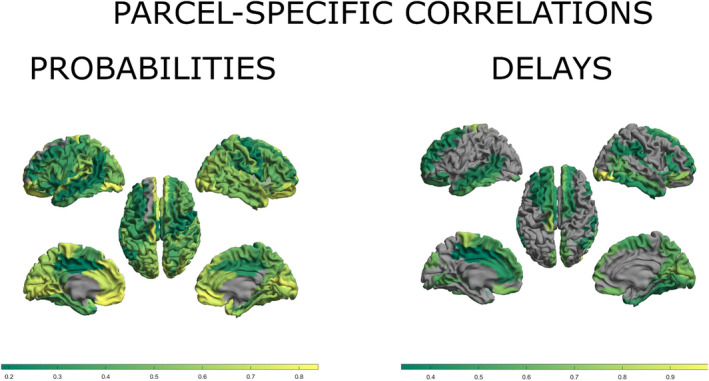
Intermodal consistency grouped by the parcel of signal propagation origin. To the left, per each region, we report the average correlation, across all the incident edges, between the transition probabilities computed from the F‐TRACT and those from the MEG dataset. To the right, the same plot for delays. Gray regions correspond to regions where the correlations did not reach statistical significance (defined as p < 0.05).
3. Discussion
In this manuscript, we set out to compare properties of large‐scale functional connectivity as measured in two different modalities. Specifically, the compared maps were probabilistic connectivity and delays related to stimulus propagation. Each map was independently computed in two considered modalities.
First, probabilities and delays were provided by a recently developed technique extracting neuronal avalanches from MEG recordings. Then, the probabilities for connections and the corresponding delays were also estimated from F‐TRACT, a large dataset of intracerebral electrical brain stimulations of the human brain. Our results show that both the probabilities and the functional delays are correlated between the modalities (r = 0.56 and r = 0.3 respectively), suggesting validity of both techniques and similarity of neuronal mechanism underpinning signal propagation in either case. Grouping both datasets according to the parcel of origin of propagation (the stimulated parcel in the F‐TRACT case) and computing correlations per each such parcel showed that parcels leading to good intermodal congruence for probabilities are also likely to lead to good congruence for delays (correlation 0.39). Averaging these parcel‐specific correlations led to results greater than obtained by correlating all data once, without grouping. This difference was especially prominent for delays (0.54 vs. 0.3), revealing even higher intermodal consistency under the grouping caveat. Moreover, this difference is a result per se, suggesting that the dependence of the temporal properties of signal propagation on the stimulated parcel, as reported from the F‐TRACT database (Lemaréchal et al. 2022), shows differently for the ATM methodology. Future studies could explore this difference further.
Indeed, the two modalities are very different from a technical standpoint, and they are derived from different cohorts. The probabilities in the two considered datasets express different measures; therefore, we do not expect agreement of absolute values but rather a correlation between them. Therefore, not the absolute values found in either modality were validated, but rather their within‐modality proportions. In particular, F‐TRACT results are obtained for a given z‐threshold (see Section 4) and a change of this threshold would systematically shift all probabilities (Trebaul et al. 2018). This might explain the fact that the transition probabilities in the ATM remain higher (above ~0.45) as compared to the ones estimated from F‐TRACT. Similarly, the maximal delay measured in the ATM technique is 64 ms, whereas longer delays were observed in F‐TRACT (presumably due to polysynaptic connections). Moreover, the F‐TRACT dataset could be considered the gold standard, given the fact that the electrodes are implanted directly within the brain, which provides better spatial resolution compared to source‐reconstructed MEG. Furthermore, with respect to the delay estimation, the F‐TRACT dataset offers a well‐controlled setting because the SEEG stimulation procedure allows one to know the exact moment and characteristic of the stimulation, as well as to register a defined pulse at the recording electrodes (Lemaréchal et al. 2022). Nevertheless, the drawback of this approach lies in the fact that direct electrical stimulation differs from physiological brain activity. In fact, the amplitude of the stimulus delivered, typically in the order of 1–5 mA, is far more intense than typical neuronal inputs. Moreover, although electrodes with high rates of interictal epileptic‐like spiking were excluded from the analyses, we cannot rule out that the remaining recordings in the F‐TRACT dataset might be partly affected by pathology.
This is different from the MEG dataset, which gathers data from healthy subjects. The source‐reconstructed MEG dataset estimates spontaneously propagating perturbations with a different experimental setup and data analysis pipeline, making it unlikely that similar results might be spurious or due to a particular technique. In fact, source reconstruction in E/MEG is an ill‐posed problem: the estimated source activity holds a degree of uncertainty, which drastically rises for the estimation of deep sources. Furthermore, applying the framework of criticality, and, in particular, that of neuronal avalanches, allows us to track spontaneous perturbations that occur in the brain on the large scale (Sorrentino, Seguin et al. 2021; Shriki et al. 2013). In this sense, one tracks scale‐free perturbations spreading spontaneously on the large scale, avoiding potential confounds induced by external stimulations. Although obtained from two independent cohorts, results from the two modalities are highly similar, suggesting that the F‐TRACT dataset could be interpreted in the context of resting state in healthy individuals, because of the two following reasons. First, there is a correlation with healthy individuals despite a potential bias related to epilepsy. Second, F‐TRACT data are obtained in a stimulation paradigm, yet they resemble data obtained during resting state. Conversely, our result suggests the reliability of the noninvasive estimation of delays and probabilities obtained by tracking neuronal avalanches from resting‐state, source‐reconstructed M/EEG data. Finally, we showed a high degree of similarity between spatial and temporal characteristics of information propagation in the human brain, as governed by two distinct mechanisms, namely spontaneous neuronal avalanches and potentials evoked with stimulation.
In conclusion, in this work we mutually validated and showed congruence between two different techniques for the estimation of connection probabilities and conduction delays from whole‐brain neurophysiological data. Our findings suggest similarity of the two distinct inspected neuronal mechanisms, and they broaden the utility of each technique. As a consequence, in the future, delay and connectivity maps estimated noninvasively might extend the personalization of large‐scale models such as The Virtual Brain (Sorrentino, Petkoski et al. 2022). In fact, the state‐of‐the‐art models assume delays as scaling proportionally to white matter tract lengths. The subsequently estimated delays range differently as compared to the observed ones (Sorrentino, Petkoski et al. 2022). Similarly, these models assume all connections to be symmetric, as directionality is not known from diffusion MRI, whereas both modalities discussed in this paper provide information about connection directionality. The personalized modeling approach could be improved with the here‐considered noninvasive method of delay and directionality estimation at the single‐subject level. Furthermore, estimating the damage from the functional delays holds promise to improve the diagnostic and prognostic management of patients with neurological and, potentially, psychiatric ailments.
4. Methods
4.1. MEG Dataset
4.1.1. Participants
Fifty‐eight right‐handed and native Italian speakers were considered for the analysis. To be included in this study, all participants had to satisfy the following criteria: (a) to have no significant medical illnesses and not to abuse substances or use medications that could interfere with MEG/EEG signals; (b) to show no other major systemic, psychiatric, or neurological illnesses; and (c) to have no evidence of focal or diffuse brain damage at routine MRI. The study protocol was approved by the local Ethics Committee. All participants gave written informed consent.
4.1.2. MEG Acquisition and Preprocessing
MEG preprocessing and source reconstruction were performed as in our earlier work (Sorrentino, Rabuffo, et al. 2022). In short, the MEG registration was divided into two eyes‐closed segments of 3:30 min each. To identify the position of the head, four anatomical points and four position coils were digitized. Electrocardiogram (ECG) and electrooculogram (EOG) signals were also recorded (Gross et al. 2013). The MEG signals, after an anti‐aliasing filter, were acquired at 1024 Hz, and then, a fourth‐order Butterworth IIR band‐pass filter in the 0.5–48 Hz band was applied. To remove environmental noise, measured by the reference magnetometers, we used principal component analysis (Sadasivan and Narayana Dutt 1996). We adopted independent component analysis to clean the data from physiological artifacts (de Cheveigné and Simon 2008), such as eye blinking (if present) and heart activity (generally one component). Noisy channels were identified and removed manually by an expert rater. 47 subjects were selected for further analysis. The time series of neuronal activity was reconstructed based on the automated anatomical labeling (AAL) (Gong et al. 2009; Oostenveld et al. 2011). To do this, we used the linearly constrained minimum variance (LCMV) beamformer algorithm based on the native MRIs (Van Veen et al. 1997). Finally, we excluded the ROIs corresponding to the cerebellum because of their low reliability in MEG. All the preprocessing and the source reconstruction were performed using the Fieldtrip toolbox (Roehri et al. 2016).
4.1.3. Transition Matrices
Each source‐reconstructed signal was binned (such as to obtain a branching ratio~1) and then z‐scored and binarized, such that, at any time bin, a z‐score exceeding ±3 was set to 1 (active); all other time bins were set to 0 (inactive). An avalanche was defined as starting when any region is above threshold, and finishing when no region is active, as in our earlier work (Sorrentino, Rucco et al. 2021). The results reported refer to binning = 3, corresponding to a branching ratio of 1. An avalanche‐specific transition matrix (ATM) was calculated, where the element (i, j) represented the probability that region j was active at time t + ẟ, given that region i was active at time t, where ẟ ~ 3 ms.
4.1.4. Construction of Random Surrogates
Randomized transition matrices were generated to ensure that associations between transition probabilities and structural connectivity could not be attributed to chance. Avalanches were randomized across time, without changing the order of avalanches at each time step. We generated a total of 1000 randomized transition matrices, and the Pearson's correlation coefficient was computed between each randomized matrix and the matrices derived from the F‐TRACT dataset. This yielded a distribution of correlation coefficients under randomization. The proportion of correlation coefficients that were greater than, or equal to, the observed correlation coefficient provided a p value for the null hypothesis that the structure of the avalanches is not related to the spreading of the cortico‐cortical evoked potential as recorded in F‐TRACT.
4.1.5. Estimation of Delay Matrices From Neuronal Avalanches
The delays were estimated for each avalanche, as in our earlier work (Sorrentino, Petkoski et al. 2022). In an avalanche, from the moment region i activated, we recorded how long it took for region j to activate. These are what we considered to be delays. Hence, for each avalanche, we obtained a matrix, in which the rows and columns represented brain regions and the entries contained the delays. We then averaged across all the avalanches belonging to one subject, obtaining an average ijth delay. The average was performed disregarding zero entries since each avalanche‐specific matrix is very sparse. With this procedure, a delay matrix was built. Averaging across subjects (again discarding zero entries) yielded a group‐specific matrix.
4.2. F‐TRACT Dataset
SEEG recordings analyzed in this study come from the F‐TRACT project (https://f‐tract.eu) (David et al. 2013; Trebaul et al. 2018; Lemaréchal et al. 2022) that to this day gathered data from over 1000 patients suffering from pharmaco‐resistant epilepsies, who in the course of preparation to the brain resection surgery underwent intracerebral implantation (Valentin 2002; Cuello Oderiz et al. 2019). All patients gave consent to undergo it, as well as to share their data for research objectives under ethical guidelines of the International Review Board at INSERM (protocol number: INSERM C14‐18) for conducting international multicenter postprocessing of clinical data. Since the MEG cohort consists of only adults, we selected from the F‐TRACT dataset only patients being at least 18 years old. As a result, in the analysis, we considered 584 implantations (288 male, 291 female, 5 unspecified) from 573 unique patients (283 male, 285 female, 5 unspecified) coming from 21 centers. The average age was 33 with SD 10. In total, 2,786,513 recordings were considered, following 29,869 stimulations (73% biphasic, 27% monophasic) with 85 electrodes per stimulation on average, the average stimulating current intensity of 3.3 mA, and pulse width 1 ms.
Derivation of the connectivity atlas is described in detail elsewhere (Trebaul et al. 2018). Briefly, the procedure was as follows. In order to minimize potential epileptic effects, for each subject we discarded 20% of contacts having the highest interictal spike count rate as assessed with DELPHOS software (Roehri et al. 2016, 2017). To mitigate volume conduction effects, we re‐referenced recorded signals to bipolar montage. The signals were band‐pass filtered in the range 1–45 Hz, and responses to all pulses in a stimulation were averaged. In order to account for individual and local specificity, we z‐scored the signal using the mean and standard deviation of spontaneous fluctuations computed on the prestimulation interval [−400, −10 ms]. Responses to stimulation trespassing z‐score threshold Z = 5 within a 200 ms poststimulation time window were considered significant. Delays were obtained from significant responses as the latency passed from stimulation until the occurrence of the first peak maximum after the threshold crossing. Similarly to our earlier study (Seguin et al. 2023), for both probabilities and delays, we only consider values computed from at least 50 measurements.
AAL parcellation (Tzourio‐Mazoyer et al. 2002) allocation to SEEG electrode contacts was performed from their MNI coordinates estimated after the MNI normalization of the preoperative MRI of individual subjects, which were first coregistered with postoperative MRI or CT scans showing implanted electrodes. On the group level, we aggregated all recordings having the same source and target parcels and we derived frequentist probability for a connection as the ratio of the number of responses considered significant over the number of stimulations between these two parcels. Similarly, the group‐level delay was estimated by the median value from delays characterizing significant responses.
Conflicts of Interest
The authors declare no conflicts of interest.
Supporting information
Data S1.
Funding: The research leading to these results has received funding from the European Research Council under the European Union's Horizon 2020 research and innovation program under grant agreement no. 945539 (SGA3) and no. 785907 (SGA2); Human Brain Project, Virtual Brain cloud no. 826421, Ministero Sviluppo Economico; Contratto di sviluppo industriale “Farmaceutica e Diagnostica” (CDS 000606) and European Union “NextGenerationEU”, (Investimento 3.1.M4. C2), project IR0000011, EBRAINS‐Italy of PNRR, the European Union's Seventh Framework Programme (FP/2007‐2013)/ERC grant agreement no. 616268 F‐TRACT, and from the Agence Nationale de la Recherche grant number ANR‐21‐NEUC‐0005‐01.
Data Availability Statement
The data that support the findings of this study are available on request from the corresponding author. The data are not publicly available due to privacy or ethical restrictions.
References
- Bullmore, E. , and Sporns O.. 2009. “Complex Brain Networks: Graph Theoretical Analysis of Structural and Functional Systems.” Nature Reviews. Neuroscience 10: 186–198. [DOI] [PubMed] [Google Scholar]
- Cuello Oderiz, C. , von Ellenrieder N., Dubeau F., et al. 2019. “Association of Cortical Stimulation–Induced Seizure With Surgical Outcome in Patients With Focal Drug‐Resistant Epilepsy.” JAMA Neurology 76: 1070–1078. [DOI] [PMC free article] [PubMed] [Google Scholar]
- David, O. , Bastin J., Chabardès S., Minotti L., and Kahane P.. 2010. “Studying Network Mechanisms Using Intracranial Stimulation in Epileptic Patients.” Frontiers in Systems Neuroscience 4: 148. [DOI] [PMC free article] [PubMed] [Google Scholar]
- David, O. , Job A. S., de Palma L., Hoffmann D., Minotti L., and Kahane P.. 2013. “Probabilistic Functional Tractography of the Human Cortex.” NeuroImage 80: 307–317. [DOI] [PubMed] [Google Scholar]
- de Cheveigné, A. , and Simon J. Z.. 2008. “Denoising Based on Spatial Filtering.” Journal of Neuroscience Methods 171: 331–339. [DOI] [PMC free article] [PubMed] [Google Scholar]
- Deco, G. , Jirsa V., McIntosh A. R., Sporns O., and Kötter R.. 2009. “Key Role of Coupling, Delay, and Noise in Resting Brain Fluctuations.” Proceedings of the National Academy of Sciences of the United States of America 106: 10302–10307. [DOI] [PMC free article] [PubMed] [Google Scholar]
- Deco, G. , Jirsa V. K., and McIntosh A. R.. 2011. “Emerging Concepts for the Dynamical Organization of Resting‐State Activity in the Brain.” Nature Reviews. Neuroscience 12: 43–56. [DOI] [PubMed] [Google Scholar]
- Gong, G. , He Y., Concha L., et al. 2009. “Mapping Anatomical Connectivity Patterns of Human Cerebral Cortex Using In Vivo Diffusion Tensor Imaging Tractography.” Cerebral Cortex 1991, no. 19: 524–536. [DOI] [PMC free article] [PubMed] [Google Scholar]
- Gross, J. , Baillet S., Barnes G. R., et al. 2013. “Good Practice for Conducting and Reporting MEG Research.” NeuroImage 65: 349–363. [DOI] [PMC free article] [PubMed] [Google Scholar]
- Lemaréchal, J.‐D. , Jedynak M., Trebaul L., et al. 2022. “A Brain Atlas of Axonal and Synaptic Delays Based on Modelling of Cortico‐Cortical Evoked Potentials.” Brain: A Journal of Neurology 145: 1653–1667. [DOI] [PMC free article] [PubMed] [Google Scholar]
- Maier‐Hein, K. H. , Neher P. F., Houde J. C., et al. 2017. “The Challenge of Mapping the Human Connectome Based on Diffusion Tractography.” Nature Communications 8: 1349. [DOI] [PMC free article] [PubMed] [Google Scholar]
- Oostenveld, R. , Fries P., Maris E., and Schoffelen J.‐M.. 2011. “FieldTrip: Open Source Software for Advanced Analysis of MEG, EEG, and Invasive Electrophysiological Data.” Computational Intelligence and Neuroscience 2011: 156869. [DOI] [PMC free article] [PubMed] [Google Scholar]
- Polverino, A. , Troisi Lopez E., Minino R., et al. 2022. “Flexibility of Fast Brain Dynamics and Disease Severity in Amyotrophic Lateral Sclerosis.” Neurology 99: e2395–e2405. 10.1212/WNL.0000000000201200. [DOI] [PMC free article] [PubMed] [Google Scholar]
- Roehri, N. , Lina J.‐M., Mosher J. C., Bartolomei F., and Benar C.‐G.. 2016. “Time‐Frequency Strategies for Increasing High‐Frequency Oscillation Detectability in Intracerebral EEG.” IEEE Transactions on Biomedical Engineering 63: 2595–2606. [DOI] [PMC free article] [PubMed] [Google Scholar]
- Roehri, N. , Pizzo F., Bartolomei F., Wendling F., and Bénar C.‐G.. 2017. “What Are the Assets and Weaknesses of HFO Detectors? A Benchmark Framework Based on Realistic Simulations.” PLoS One 12: e0174702. [DOI] [PMC free article] [PubMed] [Google Scholar]
- Sadasivan, P. K. , and Narayana Dutt D.. 1996. “SVD Based Technique for Noise Reduction in Electroencephalographic Signals.” Signal Processing 55: 179–189. [Google Scholar]
- Sanz‐Leon, P. , Knock S. A., Spiegler A., and Jirsa V. K.. 2015. “Mathematical Framework for Large‐Scale Brain Network Modeling in the Virtual Brain.” NeuroImage 111: 385–430. [DOI] [PubMed] [Google Scholar]
- Seguin, C. , Jedynak M., David O., Mansour S., Sporns O., and Zalesky A.. 2023. “Communication Dynamics in the Human Connectome Shape the Cortex‐Wide Propagation of Direct Electrical Stimulation.” Neuron 111: 1391–1401.e5. [DOI] [PubMed] [Google Scholar]
- Shriki, O. , Alstott J., Carver F., et al. 2013. “Neuronal Avalanches in the Resting MEG of the Human Brain.” Journal of Neuroscience 33: 7079–7090. [DOI] [PMC free article] [PubMed] [Google Scholar]
- Sorrentino, P. , Petkoski S., Sparaco M., et al. 2022. “Whole‐Brain Propagation Delays in Multiple Sclerosis, a Combined Tractography—Magnetoencephalography Study.” Journal of Neuroscience 42: 8807–8816. 10.1523/JNEUROSCI.0938-22.2022. [DOI] [PMC free article] [PubMed] [Google Scholar]
- Sorrentino, P. , Rabuffo G., Baselice F., et al. 2022. “Dynamical Interactions Reconfigure the Gradient of Cortical Timescales.” Network Neuroscience 1–13: 73–85. 10.1162/netn_a_00270. [DOI] [PMC free article] [PubMed] [Google Scholar]
- Sorrentino, P. , Rucco R., Baselice F., et al. 2021. “Flexible Brain Dynamics Underpins Complex Behaviours as Observed in Parkinson's Disease.” Scientific Reports 11: 4051. [DOI] [PMC free article] [PubMed] [Google Scholar]
- Sorrentino, P. , Seguin C., Rucco R., et al. 2021. “The Structural Connectome Constrains Fast Brain Dynamics.” eLife 10: e67400. [DOI] [PMC free article] [PubMed] [Google Scholar]
- Trebaul, L. , Deman P., Tuyisenge V., et al. 2018. “Probabilistic Functional Tractography of the Human Cortex Revisited.” NeuroImage 181: 414–429. [DOI] [PMC free article] [PubMed] [Google Scholar]
- Tzourio‐Mazoyer, N. , Landeau B., Papathanassiou D., et al. 2002. “Automated Anatomical Labeling of Activations in SPM Using a Macroscopic Anatomical Parcellation of the MNI MRI Single‐Subject Brain.” NeuroImage 15: 273–289. [DOI] [PubMed] [Google Scholar]
- Valentin, A. 2002. “Responses to Single Pulse Electrical Stimulation Identify Epileptogenesis in the Human Brain In Vivo.” Brain 125: 1709–1718. [DOI] [PubMed] [Google Scholar]
- Van Veen, B. D. , Van Drongelen W., Yuchtman M., and Suzuki A.. 1997. “Localization of Brain Electrical Activity via Linearly Constrained Minimum Variance Spatial Filtering.” IEEE Transactions on Biomedical Engineering 44: 867–880. [DOI] [PubMed] [Google Scholar]
Associated Data
This section collects any data citations, data availability statements, or supplementary materials included in this article.
Supplementary Materials
Data S1.
Data Availability Statement
The data that support the findings of this study are available on request from the corresponding author. The data are not publicly available due to privacy or ethical restrictions.