Genome Association Studies of Complex Diseases by Case-Control Designs

Abstract

One way to perform linkage-disequilibrium (LD) mapping of genetic traits is to use single markers. Since dense marker maps—such as single-nucleotide polymorphism and high-resolution microsatellite maps—are available, it is natural and practical to generalize single-marker LD mapping to high-resolution haplotype or multiple-marker LD mapping. This article investigates high-resolution LD-mapping methods, for complex diseases, based on haplotype maps or microsatellite marker maps. The objective is to explore test statistics that combine information from haplotype blocks or multiple markers. Based on two coding methods, genotype coding and haplotype coding, Hotelling’s T² statistics T_G and T_H are proposed to test the association between a disease locus and two haplotype blocks or two markers. The validity of the two T² statistics is proved by theoretical calculations. A statistic T_C, an extension of the traditional χ² method of comparing haplotype frequencies, is introduced by simply adding the χ² test statistics of the two haplotype blocks together. The merit of the three methods is explored by calculation and comparison of power and of type I errors. In the presence of LD between the two blocks, the type I error of T_C is higher than that of T_H and T_G, since T_C ignores the correlation between the two blocks. For each of the three statistics, the power of using two haplotype blocks is higher than that of using only one haplotype block. By power comparison, we notice that T_C has higher power than that of T_H, and T_H has higher power than that of T_G. In the absence of LD between the two blocks, the power of T_C is similar to that of T_H and higher than that of T_G. Hence, we advocate use of T_H in the data analysis. In the presence of LD between the two blocks, T_H takes into account the correlation between the two haplotype blocks and has a lower type I error and higher power than T_G. Besides, the feasibility of the methods is shown by sample-size calculation.

Introduction

With the development of the Human Genome Project and of high-resolution microsatellite and early chromosomewide haplotype maps of the human genome, enormous amounts of genetic data on human chromosomes are becoming available. The opportunities for genomewide scans to map complex-disease genes are tremendous. However, it is not yet clear how to extract the most useful information for mapping complex-disease genes. To fully utilize the massive amount of genetic data for mapping complex-disease genes, novel mathematical and statistical methods are crucial. One urgent need is to explore statistical approaches of high-resolution haplotype or multiple-marker linkage disequilibrium (LD) mapping of complex diseases. One way to perform LD mapping of genetic traits is to use single markers. Since dense marker maps—such as single-nucleotide polymorphism (SNP) and high-resolution microsatellite maps—are available (Broman et al. 1998; The International SNP Map Work Group 2001; Kong et al. 2002), it is natural and practical to generalize single-marker LD mapping to high-resolution haplotype or multiple-marker LD mapping. With the recent discovery of haplotype block structures in the human genome and with the development of early chromosomewide haplotype maps, it is important to develop better statistical methods for analysis of data on SNPs, haplotype patterns, and related patterns of LD. The chromosomewide haplotype maps are expected to be key resources for mapping complex-disease genes. For example, a systematic case-control analysis of common haplotype variants in the human genome would reveal major causative genetic contributions to a disease.

For a case-control study, one can use a χ² statistic to test the null hypothesis that the marker allele or haplotype frequencies are equal in the cases and controls on the basis of a multiple-allele marker (Olson and Wijsman 1984; Chapman and Wijsman 1998; Nielsen et al. 1998; Kaplan and Morris 2001). The method, however, can not be directly used for multiple markers or haplotype blocks, since the phase of a double heterozygote may be unknown (Ott 1999, p. 7). For multiple biallelic markers, such as SNPs, Xiong et al. (2002) proposed a Hotelling’s T² statistic for LD mapping of qualitative traits for case-control studies, which can not be used for haplotype block data with multiple haplotypes. Hence, it is necessary to develop methods of genomic LD mapping of qualitative trait loci based on haplotype block data or multiple-marker data for case-control studies.

This paper investigates methods of high-resolution LD mapping for complex diseases based on haplotype maps or microsatellite marker maps. The objective is to explore test statistics that combine information from haplotype blocks or multiple markers. For uniformity of notation, we use “haplotype blocks” or simply “blocks” in our analysis, which can be changed to “multiallelic markers.” We are interested in developing statistical methods for efficient use of genomic patterns of LD to identify genetic variants that contribute to qualitative complex diseases on the basis of multiallelic markers or haplotype block data in a case-control study. Based on two coding methods, genotype coding and haplotype coding, we propose Hotelling’s T² statistics to test the association between a disease locus and two haplotype blocks. The statistical property of the above T² statistics will be investigated. An extension of traditional χ² method of comparing haplotype frequencies is proposed by simply adding two χ² test statistics of the two haplotype blocks together. The merit of the three methods will be explored by calculation and comparison of power and type I errors. Also, the feasibility of the methods is shown by calculation of sample sizes.

Methods

Test Statistics

Suppose that a disease locus D is flanked by two haplotype blocks H₁ and H₂, where H₁ is a haplotype block on the left-hand side of D and H₂ is a haplotype block on the right-hand side. Let us denote the haplotypes of block H₁ by H₁₁,…,H_1l and the haplotypes of block H₂ by H₂₁,…,H_2r, where l and r denote the number of observed haplotypes of blocks H₁ and H₂, respectively. Consider a case-control design with N cases from an affected population and M controls from a unaffected population. Let us define a coding vector for each case or control by one of the following two ways (Schaid 1996, p. 430).

Genotype coding

For the ith case, let Hap_1i be his/her two haplotypes at block H₁, and let Hap_2i be his/her two haplotypes at block H₂. Depending on the haplotypes Hap_1i (or Hap_2i), let us define an indicator vector X_1i (or X_2i) that contains exactly one component with value 1 and other components with value 0. That is, X_1i=[x_1i1,…,x_1i(l-1),x_1i12,…,x_1i1l,…,x_1i(l-1)l]^τ, X_2i=[x_2i1,…,x_2i(r-1),x_2i12,…,x_2i1r,…,x_2i(r-1)r]^τ, and

where the indicator variables x_1ij, x_1ijk,j<k, x_2is, and x_2ist,s<t are defined by

The dimension of X_1i (or X_2i) is l(l+1)/2-1 (or r(r+1)/2-1)—that is, the total number l(l+1)/2 (or r(r+1)/2) of genotypes of haplotype block H₁ (or H₂) minus 1 to remove the redundancy.

Haplotype coding

Define X_i=[z_1i1,…,z_1i(l-1),z_2i1,…,z_2i(r-1)]^τ, where z_uij is the number of haplotypes H_uj for the ith case, i.e.,

For the ith control, one may define a vector Y_i in the same way. To illustrate the above coding methods, table1 gives an example of genotype and haplotype codings for a block H₁ with three haplotypes. The coding method for block H₂ is similar.

Table 1.

Genotype and Haplotype Codings for a Block H₁ with Three Haplotypes

	Coding for Method
Hap1i	Genotype Coding	Haplotype Coding
H11H11	10000	20
H12H12	01000	02
H13H13	00000	00
H11H12	00100	11
H11H13	00010	10
H12H13	00001	01

Let and be the mean vectors. Define a pooled-sample variance-covariance matrix by

A Hotelling’s T² statistic can be defined as

(Hotelling 1931; Anderson 1984). Hereafter, we will denote the Hotelling’s T² for haplotype coding as T_H and the Hotelling’s T² for genotype coding as T_G. Assume that the sample sizes N and M are sufficiently large that the large-sample theory applies. Under the null hypothesis of no association, the statistic T_H (or T_G) is asymptotically distributed as central χ² with l+r-2 (or [l(l+1)/2-1]+[r(r+1)/2-1]) df. Under the alternative hypothesis of association, T_H (or T_G) is asymptotically distributed as noncentral χ². If only one haplotype block H₁ is used in the analysis, the Hotelling’s T² for haplotype coding will be denoted as T_H1, and the Hotelling’s T² for genotype coding will be denoted as T_G1. Under the null hypothesis of no association, the statistic T_H1 (or T_G1) is asymptotically distributed as central χ² with l-1 (or l(l+1)/2-1) df. Under the alternative hypothesis of association, T_H1 (or T_G1) is asymptotically distributed as noncentral χ². Similarly, one may introduce test statistics T_H2 (or T_G2) if only one haplotype block H₂ is used in the analysis.

If each of haplotype block H_u has only two haplotypes H_u1,H_u2,u=1,2, then the Hotelling’s T² by haplotype coding described above coincides with the test statistic introduced by Xiong et al. (2002). To see this, notice that z_ui1=1+(z_ui1-1), where z_ui1-1 is equal to the indicator variable X_ij (defined in Xiong et al. [2002], p. 1257). Hence, our method generalizes the method of using two biallelic markers in Xiong et al. (2002) to two haplotype blocks with multiple haplotypes.

In the definition above, we consider only two haplotype blocks H₁ and H₂. In practice, the test statistics T_H and T_G can be easily generalized to multiple haplotype blocks. To make the notation as simple as possible, we will focus on two haplotype blocks throughout the present article. In appendices A, B, and C, we will justify the use of the Hotelling’s T² as an appropriate statistic to test association between the disease locus and the haplotype blocks by either the genotype coding method or the haplotype coding method. The basic idea is to show that the expectation of difference is equal to 0 if there is no association between the disease locus and the haplotype blocks. Then one may construct a test statistic based on the difference vector , which leads to the Hotelling’s T².

Noncentrality Parameters

Let Σ_A1=Cov{[z_1i1,…,z_1i(l-1)]|Aff} and Σ_A2=Cov{[z_2i1,…, z_2i(r-1)]|Aff} be variance-covariance matrices of vectors [z_1i1,…,z_1i(l-1)]^τ and [z_2i1,…,z_2i(r-1)]^τ, respectively, in affected individuals. Similarly, let z_1i(l-1)]|Unaff} and z_2i(r-1)]|Unaff} be variance-covariance matrices of column vectors [z_1i1,…,z_1i(l-1)]^τ and [z_2i1,…,z_2i(r-1)]^τ in controls. Let (or ) be the column vector of measures of LD between haplotype block H₁ (or H₂) and the disease locus D. Let α_D be the average effect of gene substitution and , and let A be the disease prevalence in population and (appendix A). Based on E(z_uij|Aff) and E(z_uij|Unaff), given in equation (A5) of appendix A, the noncentrality parameter λ_Hu of Hotelling’s test statistic T_Hu is given by

The elements of variance-covariance matrices Σ_Au and are calculated in appendix D. If the haplotype H_u has only two haplotypes—H_u1,H_u2 and N=M—then λ_Hu = 4NΔ²_u1(α_D/A − + Var(z_ui1|Unaff)]^-1, where Var(z_ui1|Aff) and Var(z_ui1|Unaff) are given in equations (D1) and (D2) in appendix D.

Let Σ_A=Cov{[z_1i1,…,z_1i(l-1),z_2i1,…,z_2i(r-1)]|Aff} be a variance-covariance matrix of column vector [z_1i1,…,z_1i(l-1),z_2i1,…,z_2i(r-1)]^τ in affected individuals. Similarly, let Unaff} be a variance-covariance matrix of column vector [z_1i1,…,z_1i(l-1),z_2i1,…,z_2i(r-1)]^τ in controls. Let us denote

Then the noncentrality parameter λ_H of Hotelling’s test statistic T_H is given by

The elements of variance-covariance matrices Σ_A and are calculated in appendices D and E. The noncentrality parameter λ_G (or λ_G1 or λ_G2) of T_G (or T_G1 or T_G2) is given in appendix F.

For a case-control study using only one haplotype block H₁, one may use a χ² statistic to test the null hypothesis that the haplotype frequencies are equal in the cases and controls (Olson and Wijsman 1994; Chapman and Wijsman 1998; Kaplan and Morris 2001). Assume that N cases and N controls are sampled. Then the test statistic is given by , where is the frequency of haplotype H_1j in the cases, and is the frequency of haplotype H_1j in the controls. Using haplotype block H₂, one may construct a similar test statistic , where is the frequency of haplotype H_2j in the cases, and is the frequency of haplotype H_2j in the controls. Using both haplotype blocks H₁ and H₂, one may construct a test statistic T_C=T_C1+T_C2 by summing T_C1 and T_C2 together. If the two statistics T_C1 and T_C2 are independent, T_C is asymptotically distributed as central χ²_l+r-2, with l+r-2 df under the null hypothesis of no association. Under the alternative hypothesis, it is asymptotically distributed as noncentral χ²_l+r-2(λ_C), where λ_C=λ_C1+λ_C2,

and +2P(H_2j)]. To calculate λ_C1, one needs to notice that P(H_1j|Aff)=E(z_1ij|Aff)/2, and so the conditional expected frequencies P(H_1j|Aff)=Δ_1jα_D/A+P(H_1j) and (appendices A and C). However, the independence of T_C1 and T_C2 can be true only in the case that there is linkage equilibrium between the two blocks. Hence, T_C may not be a valid test statistic unless one has strong evidence that the two blocks are in linkage equilibrium.

Results

Type I Errors

To explore the performance of the test statistics, we calculate type I errors for statistics T_C, T_H, and T_G for the four scenarios in table 2. We simulate 10,000 samples under an assumption of penetrance probabilities (f_DD,f_Dd,f_dd)=(0.05,0.05,0.05), which implies that the disease is not associated with the two haplotype blocks. Every sample contains 100 cases and 100 controls (N=M=100). For each sample, we calculate the empirical test statistics T_C, T_H, and T_G. The type I error is calculated by dividing the count of those empirical test statistics, which are greater than or equal to the cut-off point at the significance level α=0.01, by 10,000. We repeat the above process a total of 100 times to get 101 type I errors for each of the test statistics T_C, T_H, and T_G for the four models in table 2. On the basis of the 101 type I errors of each statistic, we calculate their mean, standard deviation (SD), minimum, and maximum, which are presented in table 2. For model I in table 2, a strong LD between the two blocks H₁, l=2, and H₂, r=2, is assumed (Δ_H11H21=0.20); in this case, the type I error of T_C (mean 0.026) is much greater than those of T_H (mean 0.011) and T_G (0.012). In model II in table 2, we assume that block H₁ has two haplotypes and the block H₂ has three haplotypes, and the measures of LD are Δ_H11H21=0.15 and Δ_H11H22=-0.075; in this case, the type I error of T_C (mean 0.017) is the highest, and T_G (mean 0.015) has higher type I error than T_H (mean 0.012). In models III and IV of table 2, the block H₂ has four haplotypes; in model III, the measures of LD are Δ_H11H21=Δ_H11H22=0.075 and Δ_H11H23=Δ_H11H24=-0.075, and in model IV, the two blocks are in linkage equilibrium; in these two cases, the type I errors of T_G (mean 0.20) are the highest, which may be due to the large degree of freedom of T_G. With LD (model III), T_C (mean 0.16) has a slightly higher type I error than T_H (mean 0.13); without LD (model VI), T_H (mean 0.013) has a slightly higher type I error than T_C (mean 0.010). Figure 1 shows the QQ plot for each statistic of T_C, T_H, and T_G for the four models in table 2. Each of the QQ plots in figure 1 is drawn by comparing 10,000 sample statistic values with 10,000 related χ²-distribution values (X-axis). These QQ plots are consistent with the results of table 2. Moreover, it is evident that the type I error level of statistic T_H is reasonable for N=M=100.

Table 2.

Type I Errors at Significance Level α=0.01 using Two Haplotype Blocks H₁, l=2, P(H₁₁)=P(H₁₂)=0.50 and H₂ with N=M=100

		Type I Error
ModelandTest	Sizea	Mean	SD	Minimum	Maximum
I:b
TG	101	.012	.001	.009	.014
TH	101	.011	.001	.008	.014
TC	101	.026	.001	.022	.030
II:c
TG	101	.015	.001	.012	.018
TH	101	.012	.001	.010	.015
TC	101	.017	.001	.014	.021
III:d
TG	101	.020	.001	.018	.023
TH	101	.013	.001	.011	.015
TC	101	.016	.001	.012	.018
IV:e
TG	101	.020	.001	.016	.023
TH	101	.013	.001	.011	.016
TC	101	.010	.001	.007	.012

^aSize is the total number of type I errors calculated for each statistic under a specific model.

^bIn model I, r=2, P(H₂₁)=P(H₂₂)=0.50, and Δ_H11H21=-Δ_H11H22=0.20.

^cIn model II, r=3, P(H₂₁)=0.4,P(H₂₂)=P(H₂₃)=0.30, Δ_H11H21=0.15, and Δ_H11H22=Δ_H11H23=-0.075.

^dIn model III, r=4, P(H₂₁)=P(H₂₂)=P(H₂₃)=P(H₂₄)=0.25, Δ_H11H21=P(H₁₁H₂₁)-P(H₁₁)P(H₂₁)=0.075, Δ_H11H22=P(H₁₁H₂₂)-P(H₁₁)P(H₂₂)=0.075, Δ_H11H23=P(H₁₁H₂₃)-P(H₁₁)P(H₂₃)=-0.075, and Δ_H11H24=P(H₁₁H₂₄)-P(H₁₁)P(H₂₄)=-0.075.

^eIn model IV, all parameters are the same as those of model III, except that Δ_H11H21=Δ_H11H22=Δ_H11H23=Δ_H11H24=0.

Figure 1.

QQ plot at significance level α=0.01 using two haplotype blocks H₁, l=2, and H₂. In graphs I.1, I.2, and I.3, all parameters are the same as those of model I in table 2. In graphs II.1, II.2, and II.3, all parameters are the same as those of model II in table 2. In graphs III.1, III.2, and III.3, all parameters are the same as those of model III in table 2. In graphs IV.1, IV.2, and IV.3, all parameters are the same as those of model IV in table 2.

Power Calculation and Comparison

To calculate the noncentrality parameters, we assume a deterministic population genetic model. Assume that a single disease mutation was introduced into the population T generations ago, with a frequency P_D. First, we consider only one haplotype block H_u, u=1,2. At the initial generation of the occurrence of the mutation, the haplotype frequencies P(H_u1D)(0)=P_D and P(H_ujD)(0)=0,j=2,…, l, if u=1, or j=2,…, r,if u=2. Moreover, P(H_u1d)(0)=P(H_u1)-P_D and P(H_ujd)(0)=P(H_uj),j=2,…,l if u=1, or j=2,…,r if u=2. Let θ_u be the recombination fraction between haplotype block H_u and disease locus D,u=1,2. Given a map distance λ_u between haplotype block H_u and disease locus D, the recombination fraction θ_u can be calculated by Haldane’s map function θ_u=[1-exp(-2λ_u)]/2, under the assumption of no interference. At generation T, the haplotype frequencies can be approximately calculated by P(H_ujD)(T)=P(H_ujD)(0)e^-Tθ_u+P_DP(H_uj)(1-e^-Tθ_u) and P(H_ujd)(T)=P(H_ujd)(0)e^-Tθ_u+P_dP(H_uj)(1-e^-Tθ_u),j=1,…,l, if u=1, or j=2,…,r, if u=2. Second, we consider both haplotype blocks H₁ and H₂. At the initial generation of the occurrence of mutation, the haplotype frequencies P(H₁₁DH₂₁)(0)=P_D and P(H_1jDH_2s)(0)=0,j=1,…,l,s=1,…,r, and (j,s)≠(1,1). That is, the disease-susceptibility allele D was carried by haplotype H₁₁H₂₁ at the initial generation of mutation. The other initial haplotype frequencies are P(H₁₁dH₂₁)(0)=P(H₁₁H₂₁)-P_D and P(H_1jdH_2s)(0)=P(H_1jH_2s),j=1,…,l,s=1,…,r and (j,s)≠(1,1).

At generation T, the haplotype frequencies can be approximately calculated by P(H_1jDH_2s)(T)=Δ_jDs(0)e^{-T(θ₁+θ₂)} + P(H_1j)Δ_2s(0)e^-Tθ₂ + P(H_2s)Δ_1j(0)e^-Tθ₁+ P(H_1j)P_DP(H_2s) and P(H_1jdH_2s)(T)=P(H_1jH_2s)-P(H_1jDH_2s)(T),j=1,…, l, s=1,…, r, where Δ_jDs(0) = P(H_1jDH_2s)(0) − P(H_1j)Δ_2s(0) − P(H_2s)Δ_1j(0) − P(H_1j)P_DP(H_2s) is the measure of initial LD at the three loci for haplotypes H_1j and H_2s, Δ_1j(0)=P(H_1jD)(0)-P(H_1j)P_D is the measure of initial LD between haplotype H_1j and disease locus D, and Δ_2s(0)=P(DH_2s)(0)-P_DP(H_2s) is the measure of initial LD between haplotype H_2s and disease locus D (Akey et al. 2001).

To make a power comparison, we consider four genetic models: heterogeneous recessive, heterogeneous dominant, additive, and multiplicative. First, we consider optimistic penetrance probabilities and genotype relative risks given in table 3 (Nielson et al. 1998). For less optimistic models, with lower penetrance probabilities and genotype relative risks, we consider the four models in table 4. For each model in table 4, the population disease prevalence is ∼0.05 and the sib recurrence risk is ∼0.06 (Iles 2002). We assume that the distance between the two haplotype blocks is 4 cM. The block H₁ is located at position 0 cM, and the block H₂ is located at position 4 cM. Since the disease locus D is usually unknown, we assume that it is located in the interval between H₁ and H₂. Given the location of disease locus D, the map distance λ_u between H_u and D can be used to calculate the recombination fraction θ_u by Haldane’s map function, u=1,2, λ₁+λ₂=4 cM. To calculate the power, we first partition the interval of 4 cM between block H₁ and H₂ to be 100 subintervals with 101 end-points. Given that the disease locus D is located at an end-point, we may perform power calculation at this locus. We assume that the haplotype H₁ has two haplotypes H₁₁ and H₁₂ with equal frequencies, P_D=0.10, N=M=100, and T=50 for the four models in table 3. For the four models in table 4, P_D=0.30, N=M=500. For each genetic model in table 4, figures 2, 3, and 4 show power curves of T_C,T_H,T_G,T_C2,T_H2, and T_G2 for r=2,3,4 haplotypes of block H₂, respectively. The related parameters, such as measures of LD between block H₁ and block H₂, are given in the legend of each figure. First, it is clear from these three figures that the power of using two haplotype blocks is generally higher than that of using one block. When the disease locus D is far from block H₂, the power of using two haplotype blocks is significantly higher. When the disease locus D is close to block H₂, the power of using two haplotype blocks is similar to that of using only one block H₂. Second, the power of T_C is generally higher than or similar to that of T_H, and the power of T_H is higher than or similar to that of T_G. This may be due to the lack of consideration of correlation between the two blocks by T_C (see the type I error comparison in table 2). Third, the power of T_C2 is similar to that of T_H2 and higher than that of T_G2.

Table 3.

First Set of Parameters of Simulated Genetic Models

Model Type	fDD	fDd	fdd
Heterogeneous recessive	1.00	.05	.05
Heterogeneous dominant	1.00	.95	.05
Additive	1.00	.50	.0
Multiplicative	.81	.045	.0025

Table 4.

Second Set of Parameters of Simulated Genetic Models

Model Type	fDD	fDd	fdd
Heterogeneous recessivea	.16	.04	.04
Heterogeneous dominantb	.08	.08	.02
Additivec	.108	.0675	.027
Multiplicatived	.12	.06	.03

^af_DD=4f_Dd=4f_dd.

^bf_DD=f_Dd=4f_dd.

^cf_DD=4f_dd, f_Dd=(f_DD+f_dd)/2.

^df_DD=4f_dd, f_Dd=2f_dd.

Figure 2.

Power curves of T_C, T_H, T_G, T_C2, T_H2, and T_G2 at significance level α=0.01, using two haplotype blocks H₁, l=2, and H₂, r=2, when P(H₁₁)=P(H₁₂)=P(H₂₁)=P(H₂₂)=0.50, Δ_H11H21=P(H₁₁H₂₁)-P(H₁₁)P(H₂₁)=0.075, Δ_H11H22=P(H₁₁H₂₂)-P(H₁₁)P(H₂₂)=-0.075, P_D=0.30, N=M=500, T=50, for the four genetic models in table 4.

Figure 3.

Power curves of T_C, T_H, T_G, T_C2, T_H2, and T_G2 at significance level α=0.01, using two haplotype blocks H₁, l=2, and H₂, r=3, when P(H₁₁)=P(H₁₂)=0.5, P(H₂₁)=0.4, P(H₂₂)=P(H₂₃)=0.30, Δ_H11H21=P(H₁₁H₂₁)-P(H₁₁)P(H₂₁)=0.075, Δ_H11H22=P(H₁₁H₂₂)-P(H₁₁)P(H₂₂)=-0.0375, Δ_H11H23=P(H₁₁H₂₃)-P(H₁₁)P(H₂₃)=-0.0375, P_D=0.30,N=M=500,T=50, for the four genetic models in table 4.

Figure 4.

Power curves of T_C, T_H, T_G, T_C2, T_H2, and T_G2 at significance level α=0.01 using two haplotype blocks H₁, l=2, and H₂, r=4, when P(H₁₁)=P(H₁₂)=0.5,P(H₂₁)=P(H₂₂)=P(H₂₃)=P(H₂₄)=0.25, Δ_H11H21=P(H₁₁H₂₁)-P(H₁₁)P(H₂₁)=0.075, Δ_H11H22=P(H₁₁H₂₂)-P(H₁₁)P(H₂₂)=0.075, Δ_H11H23=P(H₁₁H₂₃)-P(H₁₁)P(H₂₃)=-0.075, Δ_H11H24=P(H₁₁H₂₄)-P(H₁₁)P(H₂₄)=-0.075, P_D=0.30, N=M=500, T=50, for the four genetic models in table 4.

To explore the effect of the degree of LD on the test statistics, figure 5 plots power curves under an assumption of linkage equilibrium between the two blocks H₁ and H₂ for four models in table 4. From the four graphs of figure 5, the power of T_H is similar to or slightly higher than that of T_C, except for heterogeneous recessive and multiplicative models, in which the power of T_H is slightly lower than that of T_C. In all graphs of figure 5, the power of T_C and T_H is higher than that of T_G. Figure 6 plots power curves for different mutation ages of the disease allele D for four models in table 4. For the four models in table 4, the power is very high for a disease mutation of T=30, high for T=40, and relatively high for T=50 generations old. Figure 7 plots power curves of T_H for different disease frequencies P_D for the four models in table 4. For recessive disease model in table 4, a disease with frequency P_D⩾0.30 would have high power if the haplotype block is close to the disease locus. For the other three models in table 4, a disease with frequency P_D⩾0.20 would have high power if the haplotype block is close to the disease locus (fig. 7).

Figure 5.

Power curves of T_C, T_H, and T_G at significance level α=0.01 using two haplotype blocks H₁, l=2, and H₂, r=4, when P(H₁₁)=P(H₁₂)=0.5,P(H₂₁)=P(H₂₂)=P(H₂₃)=P(H₂₄)=0.25, Δ_H11H21=P(H₁₁H₂₁)-P(H₁₁)P(H₂₁)=0.0, Δ_H11H22=P(H₁₁H₂₂)-P(H₁₁)P(H₂₂)=0.0, Δ_H11H23=P(H₁₁H₂₃)-P(H₁₁)P(H₂₃)=0.0, Δ_H11H24=P(H₁₁H₂₄)-P(H₁₁)P(H₂₄)=0.0, P_D=0.30, N=M=500, T=50, for the four genetic models in table 4.

Figure 6.

Power curves of T_H for different mutation ages at significance level α=0.01, using two haplotype blocks H₁, l=2, and H₂, r=4, when P(H₁₁)=P(H₁₂)=0.5, P(H₂₁)=P(H₂₂)=P(H₂₃)=P(H₂₄)=0.25, Δ_H11H21=P(H₁₁H₂₁)-P(H₁₁)P(H₂₁)=0.075, Δ_H11H22=P(H₁₁H₂₂)-P(H₁₁)P(H₂₂)=0.075, Δ_H11H23=P(H₁₁H₂₃)-P(H₁₁)P(H₂₃)=-0.075, Δ_H11H24=P(H₁₁H₂₄)-P(H₁₁)P(H₂₄)=-0.075, P_D=0.30, N=M=500, for the four genetic models in table 4.

Figure 7.

Power curves of T_H for different disease frequency at significance level α=0.01, using two haplotype blocks H₁, l=2, and H₂, r=4, when P(H₁₁)=P(H₁₂)=0.5, P(H₂₁)=P(H₂₂)=P(H₂₃)=P(H₂₄)=0.25, Δ_H11H21=P(H₁₁H₂₁)-P(H₁₁)P(H₂₁)=0.075, Δ_H11H22=P(H₁₁H₂₂)-P(H₁₁)P(H₂₂)=0.075, Δ_H11H23=P(H₁₁H₂₃)-P(H₁₁)P(H₂₃)=-0.075, Δ_H11H24=P(H₁₁H₂₄)-P(H₁₁)P(H₂₄)=-0.075, T=50, N=M=500, for the four genetic models in table 4.

Corresponding to the six figures for the less optimistic models in table 4, we provide six figures for the optimistic models in table 3 on our Web site. The power of the heterogeneous recessive model in table 3 is low (figs. 1, 2, and 3 on our Web site). In contrast, the power of the heterogeneous recessive model in table 4 is reasonably high (figs. 2, 3, and 4). In the absence of LD, the power of T_H is similar to or slightly higher than that of T_C for the four models in table 3 (fig. 4 on our Web site). For recessive disease model in table 3, the power is low even for very young disease mutation (T=10) (fig. 5 on our Web site). For the recessive disease model in table 3, a disease with frequency P_D⩾0.15 would have high power if the haplotype block is close to the disease locus. For the other three models in table 3, a disease with frequency P_D⩾0.10 would have high power (fig. 6 on our Web site).

Sample Size

Table 5 gives sample size required for the four genetic models in table 3 at significance level .01 and 80% power using two haplotype blocks H₁, l=2, and H₂, r=4. Except for heterozygous recessive disease with low disease-allele frequency P_D=0.05, the sample sizes required are <400 and are feasible in practice. For most cases, the sample sizes required are <100. Table 6 gives the sample sizes required for the four genetic models in table 4 at significance level 0.01 and 80% power, using two haplotype blocks H₁, l=2, and H₂, r=4. Compared with the sample sizes in table 5 for the four models in table 3, the sample sizes in table 6 for the four models in table 4 are much greater. For the recessive disease model in table 4, the sample sizes required for low frequency (P_D⩽0.10) are >5,000, and so it may not be realistic to recruit enough patients for such disease studies. For all dominant disease models and recessive disease models with high disease frequency (P_D=0.20 or 0.30), the sample sizes required are <1,000 and are feasible in practice. For the additive and multiplicative disease models in table 4, the sample sizes required are <1,000, except for low–disease-frequency cases (P_D=0.05) or old disease mutations (T⩾50).

Table 5.

Sample Sizes Required for the Four Genetic Models in Table 3, at Significance Level 0.01 and 80% Power, Using Two Haplotype Blocks H₁, l=2, and H₂, r=4^[Note]

	Required Sample Size
	T=20			T=30			T=40			T=50			T=60
Model Typeand PD	TC	TH	TG	TC	TH	TG	TC	TH	TG	TC	TH	TG	TC	TH	TG
Heterogeneous recessive:
.05	2,296	3,005	2,145	2,534	3,297	2,455	2,798	3,619	2,806	3,088	3,976	3,202	3,409	4,369	3,650
.10	193	279	241	213	303	271	235	329	303	258	358	339	285	390	379
.15	57	85	82	62	92	92	68	99	102	75	107	113	83	116	125
Heterogeneous dominant:
.05	45	47	60	50	53	67	55	59	75	60	65	84	66	73	94
.10	26	24	29	29	27	33	32	30	38	35	34	43	39	38	48
.15	19	15	17	21	17	21	23	20	24	26	23	28	28	26	32
Additive:
.05	22	18	21	25	21	24	27	24	28	30	27	32	33	31	37
.10	20	16	18	22	18	21	24	21	24	27	24	28	29	27	32
.15	18	13	15	20	16	18	22	18	21	24	20	24	26	23	28
Multiplicative:
.05	29	34	47	32	38	51	35	41	56	38	46	62	42	50	68
.10	15	17	23	17	19	25	19	21	28	21	23	31	23	25	34
.15	12	11	15	13	13	17	14	14	19	15	16	22	17	18	24

Note.— Data shown are for P(H₁₁)=P(H₁₂)=0.5, P(H₂₁)=P(H₂₂)=P(H₂₃)=P(H₂₄)=0.25, Δ_H11H21=P(H₁₁H₂₁)-P(H₁₁)P(H₂₁)=0.075, Δ_H11H22=P(H₁₁H₂₂)-P(H₁₁)P(H₂₂)=0.075, Δ_H11H23=P(H₁₁H₂₃)-P(H₁₁)P(H₂₃)=-0.075, Δ_H11H24=P(H₁₁H₂₄)-P(H₁₁)P(H₂₄)=-0.075, and θ₁=θ₂=0.005.

Table 6.

Sample Sizes Required for the Four Genetic Models in Table 4 at Significance Level 0.01 and 80% Power Using Two Haplotype Blocks H₁, l=2, and H₂, r=4^[Note]

	Required Sample Size
	T=30			T=40			T=50			T=60
Model Typeand PD	TC	TH	TG	TC	TH	TG	TC	TH	TG	TC	TH	TGc
Heterogeneous recessive:
.05	94,373	117,340	78,996	104,275	129,519	91,520	115,217	142,977	105,797	127,309	157,850	122,031
.10	6233	7965	5707	6883	8763	6555	7601	9644	7517	8394	10618	8607
.20	477	657	550	525	716	620	579	782	698	639	854	785
.30	125	183	173	138	198	192	152	215	214	167	233	238
Heterogeneous dominant:
.05	469	576	771	517	635	851	570	699	939	629	770	1,036
.10	196	233	302	216	257	335	238	284	370	262	313	410
.20	109	121	145	120	134	162	132	149	181	145	165	202
.30	93	96	104	102	107	117	112	119	133	123	133	150
Additive:
.05	1,296	1,607	2,188	1,430	1,771	2,412	1,578	1,952	2,658	1,741	2,151	2,931
.10	421	520	703	464	572	774	512	630	853	564	694	940
.20	162	195	260	178	215	287	196	237	317	216	261	350
.30	102	119	157	112	132	174	123	145	192	136	160	212
Multiplicative:
.05	2,397	2,979	4,070	2,646	3,284	4,487	2,921	3,620	4,946	3,224	3,992	5,454
.10	669	836	1,141	737	919	1,256	813	1,012	1,382	897	1,114	1,522
.20	203	254	347	224	279	382	246	307	419	271	337	460
.30	107	133	182	118	146	200	130	160	219	143	176	241

Note.— All other parameters except the penetrance probabilities are the same as those in table 5.

For the sample sizes given in tables 5 and 6, we perform an empirical power calculation by 10,000 replicates. The results for T_H are pretty consistent with the theoretical value of 0.80.

Discussion

The objective of this paper is to explore methods for high-resolution haplotype or multiple-marker genome-association studies of complex diseases by case-control designs. We investigated test statistics that combine information from haplotype blocks or multiple markers. We introduced two Hotelling’s T² statistics T_G and T_H to test association between a disease locus and two haplotype blocks on the basis of two coding methods, genotype coding and haplotype coding. By theoretical analysis, we showed that they are valid test statistics. Ignoring the correlation between the two blocks, one may use an extension sum statistic, T_C, of two traditional χ² test statistics, T_C1 and T_C2, for comparing haplotype frequencies in cases and controls. For each of the three statistics, the power of using two haplotype blocks is higher than that of using only one haplotype block. By power comparison, we notice that T_C has higher power than T_H, and T_H has higher power than T_G.

In the absence of LD between the two blocks, the power of T_C is similar to that of T_H and is higher than that of T_G. In the presence of LD between the two blocks, the type I error of T_C is higher than those of T_H and T_G. Hence, we advocate to use T_H in the data analysis. In the presence of LD between the two blocks, T_H takes into account of the correlation between the two haplotype blocks and has the lowest type I error and a higher power than T_G. On the one hand, T_G has the lowest power, although it takes into account the correlation between the two haplotype blocks. On the other hand, the type I error of T_G gets bigger as the number of haplotypes increases, which may be due to the large degree of freedom. Therefore, T_G is less favorable than T_H.

Several empirical studies showed that the haplotypes have block structures in human genome, and each haplotype block has limited diversity (Daly et al. 2001; Goldstein 2001; Patil et al. 2001; Reich et al. 2001; Rioux et al. 2001; Stephens et al. 2001; Gabriel et al. 2002). The haplotype blocks are punctuated by apparent sites of recombination or hot-spot areas. Within a haplotype block, there are only a few (2–4) haplotypes, and LD decays only gradually with distance. Within the hot-spot areas, however, there may have been several recombination events, and thus LD decays rapidly with distance. The recombination events are clustered to be hot spots. These patterns of LD are very relevant to genomewide association studies for mapping complex-disease genes. However, the general properties of haplotype structure in human genome are not fully understood. It is necessary to characterize patterns of LD in the human genome, and to investigate approaches of high resolution LD mapping of complex traits based on haplotype block data.

The test statistics, such as T_H and T_G, that are based on multiallelic markers or haplotype blocks can usually lead to a large number of df. However, when haplotype block data are used, the df would not be very large if one took into account the recent discovery of haplotype structure in human genome. Although a haplotype block may enclose many SNPs, it takes only a few SNPs to uniquely identify each of the haplotypes in the block. This implies that the number of df when haplotype block data are used may be even less than that when multiple SNP markers are used in an analysis. Moreover, haplotype block data already take into account the haplotype structure and potentially are more powerful.

In our analysis, only two haplotype blocks are discussed. One could generalize the method to use multiple haplotype blocks in the analysis. One interesting topic is to study the merit of a generalized T_H that uses multiple haplotype blocks, instead of the current version of T_H, which uses only two haplotype blocks. Moreover, the methods can be generalized to analyze pedigree data, including sib pairs (Cordell and Clayton 2002). Other issues, such as population-stratification effects and methods of combining population and pedigree data, are exciting research topics (Ardlie et al. 2000; Rannala and Reeve 2001). If the data contain individuals with missing genotypes within the haplotype blocks or with genotyping errors, some potential problems can arise in actual data analysis. The effect of uncertainty in the haplotype block’s start and stop positions is unclear. More investigations will be necessary to cope with these challenges.

Appendix A

Suppose that the disease locus has two alleles D and d, D being the allele for disease susceptibility and d being normal. Assume that the disease-susceptibility allele D has population frequency P_D, and normal allele d has population frequency P_d. Let f_DD, f_Dd=f_dD, and f_dd be the probabilities that an individual with genotypes DD, Dd, and dd is affected with the disease, respectively. Since allele D is disease susceptible, one may assume f_DD⩾f_Dd⩾f_dd. Let and . Denote the disease prevalence in the population by A=f_DDP²_D+2f_DdP_DP_d+f_ddP²_d, and . As in quantitative genetics, let us introduce some notation. Let a=f_DD-(f_DD+f_dd)/2,d=f_Dd-(f_DD+f_dd)/2, δ_D=2d, and α_D=a+(P_d-P_D)d. In terms of quantitative genetics, α_D is the average effect of gene substitution, and δ_D is the dominant deviation (Falconer and Mackay 1996). Similarly, denote , and . Denote the measures of LD between haplotype H_1j of the first haplotype block H₁ and the disease locus D by Δ_1j=P(H_1jD)-P(H_1j)P_D,j=1,…,l, and the measures of LD between haplotype H_2s of the second haplotype block H₂ and the disease locus D by Δ_2s=P(DH_2s)-P(H_2s)P_D,s=1,…,r. For u=1,2, the frequencies of heterozygous genotype H_ujH_uk,j≠k, in affected and unaffected individuals are calculated in appendix B as

The frequencies of homozygous genotype H_ujH_uj in affected and unaffected individuals are calculated in appendix B as

Under the null hypothesis of no association between the haplotype blocks H_u,u=1,2 and the disease locus D—that is, Δ_uj=0 for all j, equations (A1), (A2), (A3) and (A4), imply the expectation for genotype coding method. In appendix C, we show

Hence, we have which implies the expectation for the haplotype coding method, under the null hypothesis of no association between the haplotype blocks H_u,u=1,2 and the disease locus D.

Appendix B

Notice that P(H_ujD)=Δ_uj+P(H_uj)P_D,P(H_ujd)=-Δ_uj+P(H_uj)P_d, P(H_ukD)=Δ_uk+P(H_uk)P_D, and P(H_ukd)=-Δ_uk+P(H_uk)P_d for u=1,2. Using the expression α_D=(f_DD-f_dd)/2+(P_d-P_D)[f_Dd-(f_DD+f_dd)/2]=P_Df_DD+P_df_Dd-P_Df_Dd-P_df_dd, the frequency of genotype H_ujH_uk,j≠k, in affected can be calculated as

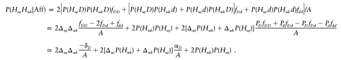Similarly, the frequency of genotype H_ujH_uj in affected can be calculated as

Similarly, we may prove equations (A2) and (A4).

Appendix C

Notice that and . From equations (A1) and (A3), the expectation of numbers of haplotypes H_uj in affected is equal to

Similarly, one may show that the expectation of numbers of haplotypes H_uj in unaffected is equal to

Appendix D

Using the notations of in equations (A1), (A2), (A3), and (A4), we calculate the variance-covariance matrices Σ_A1 and . First, we calculate the variance of the number of haplotypes H_uj in affected by equations (A3) and (A5)

Similarly, the variance of the number of haplotypes H_uj in controls is

By use of equations (A1) and (A5), the covariance between the number of haplotypes H_uj and the number of haplotypes H_uk, j≠k in affected individuals is

Similarly, the covariance between the number of haplotypes H_uj and the number of haplotypes H_uk, j≠k in controls is

Appendix E

To calculate the covariance between z_1ij,z_2is, denote for j≠k,s≠t

For j=1,…,l-1 and s=1,…,r-1, the covariance

Similarly, for j=1,…,l-1 and s=1,…,r-1, the covariance

where and are expected genotype frequencies in controls like those defined in equation (E1) for cases.

Appendix F

To calculate the noncentrality parameter λ_G, we notice first that the expectation

where is equal to , and is equal to .

Let Σ_G be the variance-covariance matrix of genotype coding X_i. Then its elements can be calculated by Var(x_uij|Aff)=a_ujj-a²_ujj, where j=1,…,l-1 if u=1 and j=1,…,r-1 if u=2, Var(x_uijk|Aff)=a_ujk-a²_ujk,j≠k, Cov(x_uij,x_ui(j+k)|Aff)=-a_ujja_u(j+k)(j+k) if k⩾1, Cov(x_uij,x_uimk|Aff)=-a_ujja_umk for m≠k, Cov(x_uijk,x_uist|Aff)=-a_ujka_ust for j≠k and s≠t.

Using the notation in equations (A1), (A3), and (E1), the covariances between x_1ij,x_1ijk and x_2is,x_2ist are given by

Similarly, we may calculate the variance-covariance matrix for the controls. Then the noncentrality parameter λ_G of T_G is given by

Using the variance-covariance matrices Σ_G1 and of the genotype coding vector X_1i in affected and unaffected individuals, one may calculate the noncentrality parameter λ_G1 similarly.

References

- Akey J, Jin L, Xiong MM (2001) Haplotype vs. single marker linkage disequilibrium tests: what do we gain? Eur J Hum Genet 9:291–300 [DOI] [PubMed] [Google Scholar]
- Anderson TW (1984) An introduction to multivariate statistical analysis, 2nd edition. John Wiley and Sons, New York [Google Scholar]
- Ardlie KG, Lunetta KL, Seielstad M (2002) Testing for population subdivision and association in four case-control studies. Am J Hum Genet 71:304–311 [DOI] [PMC free article] [PubMed] [Google Scholar]
- Broman KW, Murray JC, Sheffied VC, White RL, Weber JL (1998) Comprehensive human genetic map: individual and sex-specific variation in recombination. Am J Hum Genet 63:861–869 [DOI] [PMC free article] [PubMed] [Google Scholar]
- Chapman NH, Wijsman EM (1998) Genome screens using linkage disequilibrium tests: optimal marker characteristics and feasibility. Am J Hum Genet 63:1872–1885 [DOI] [PMC free article] [PubMed] [Google Scholar]
- Cordell HJ, Clayton DG (2002) A unified stepwise regression procedure for evaluating the relative effects of polymorphisms within a gene using case/control or family data: application to HLA in type 1 diabetes. Am J Hum Genet 70:124–141 [DOI] [PMC free article] [PubMed] [Google Scholar]
- Daly MJ, Rioux JD, Schaffner SF, Hudson TJ, Lander ES (2001) High-resolution haplotype structure in the human genome. Nat Genet 29:229–232 [DOI] [PubMed] [Google Scholar]
- Falconer DS, Mackay TFC (1996) Introduction to quantitative genetics, 4th edition. Longman, London [Google Scholar]
- Gabriel SB, Schaffner SF, Nguyen H, Moore JM, Roy J, Blumenstiel B, Higgins J, DeFelice M, Lochner A, Faggart M, Liu-Cordero SN, Rotimi C, Adeyemo A, Cooper R, Ward R, Lander ES, Daly MJ, Altshuler D (2002) The structure of haplotype blocks in the human genome. Science 296:2225–2229 [DOI] [PubMed] [Google Scholar]
- Goldstein GB (2001) Islands of LD. Nat Genet 29:109–111 [DOI] [PubMed] [Google Scholar]
- Hotelling H (1931) The generalization of student’s ratio. Ann Math Stat 2:360–378 [Google Scholar]
- Iles MM (2002) Effect of mode of inheritance when calculating the power of a transmission/disequilibrium test study. Hum Hered 53:153–157 [DOI] [PubMed] [Google Scholar]
- The International SNP Map Working Group (2001) A map of human genome sequence variation containing 1.42 million single nucleotide polymorphisms. Nature 409:928–933 [DOI] [PubMed] [Google Scholar]
- Kaplan N, Morris R (2001) Issues concerning association studies for fine mapping a susceptibility gene for a complex disease. Genet Epidemiol 20:432–457 [DOI] [PubMed] [Google Scholar]
- Kong A, Gudbjartsson DF, Sainz J, Jonsdottir GM, Gudjonsson SA, Richardsson B, Sigurdardottir S, Barnard J, Hallbeck B, Masson G, Shlien A, Palsson ST, Frigge ML, Thorgeirsson TE, Gulcher JR, Stefansson K (2002) A high resolution recombination map of the human genome. Nat Genet 31:241–247 [DOI] [PubMed] [Google Scholar]
- Nielsen DM, Ehm MG, Weir BS (1998) Detecting marker-disease association by testing for Hardy-Weinberg disequilibrium at a marker locus. Am J Hum Genet 63:1531–1540 [DOI] [PMC free article] [PubMed] [Google Scholar]
- Olson JM, Wijsman EM (1994) Design and sample size considerations in the detection of linkage disequilibrium with a marker locus. Am J Hum Genet 55:574–580 [PMC free article] [PubMed] [Google Scholar]
- Ott J (1999) Analysis of human genetic linkage, 3rd edition. Johns Hopkins University Press, Baltimore and London [Google Scholar]
- Patil NP, Berno AJ, Hinds DA, Barrett WA, Doshi JM, Hacker CR, Kautzer CR, Lee DH, Marjoribanks C, McDonough DP, Nguyen BTN, Norris MC, Sheehan JB, Shen N, Stern D, Stokowski RP, Thomas DJ, Trulson MO, Vyas KR, Frazer KA, Fodor SPA, Cox DR (2001) Blocks of limited haplotype diversity revealed by high-resolution scanning of human chromosome 21. Science 294:1719–1723 [DOI] [PubMed] [Google Scholar]
- Rannala B, Reeve JP (2001) High-resolution multipoint linkage-disequilibrium mapping in the context of a human genome sequence. Am J Hum Genet 69:159–178 (erratum 69:172) [DOI] [PMC free article] [PubMed] [Google Scholar]
- Reich DE, Cargill M, Bolk S, Ireland J, Sabett RC, Richter DJ, Lavery T, Kouyounmjian R, Farhadian SF, Ward R, Lander ES (2001) Linkage disequilibrium in the human genome. Nature 411:199–204 [DOI] [PubMed] [Google Scholar]
- Rioux JD, Daly MJ, Silverberg MS, Lindblad K, Steinhart H, Cohen Z, Delmonte T, et al (2001) Genetic variation in the 5q31 cytokine gene cluster confers susceptibility to Crohn disease. Nat Genet 29:223–228 [DOI] [PubMed] [Google Scholar]
- Schaid DJ (1996) General score tests for associations of genetic markers with disease using cases and their parents. Genet Epidemiol 13:423–449 [DOI] [PubMed] [Google Scholar]
- Schaid DJ, Rowland C (1998) Use of parents, sibs, and unrelated controls for detection of associations between genetic markers and disease. Am J Hum Genet 63:1492–1506 [DOI] [PMC free article] [PubMed] [Google Scholar]
- Stephens JC, Schneider JA, Tanguay DA, Choi J, Acharya T, Stanley SE, Jiang R, et al (2001) Haplotype variation and linkage disequilibrium in 313 human genes. Science 293:489–493 [DOI] [PubMed] [Google Scholar]
- Xiong MM, Zhao J, Boerwinkle E (2002) Generalized T2 test for genome association studies. Am J Hum Genet 70:1257–1268 [DOI] [PMC free article] [PubMed] [Google Scholar]