Fine-Scale Mapping of Disease Genes with Multiple Mutations via Spatial Clustering Techniques

Abstract

We present a method to perform fine mapping by placing haplotypes into clusters on the basis of risk. Each cluster has a haplotype “center.” Cluster allocation is defined according to haplotype centers, with each haplotype assigned to the cluster with the “closest” center. The closeness of two haplotypes is determined by a similarity metric that measures the length of the shared segment around the location of a putative functional mutation for the particular cluster. Our method allows for missing marker information but still estimates the risks of complete haplotypes without resorting to a one-marker-at-a-time analysis. The dimensionality issues that can occur in haplotype analyses are removed by sampling over the haplotype space, allowing for estimation of haplotype risks without explicitly assigning a parameter to each haplotype to be estimated. In this way, we are able to handle haplotypes of arbitrary size. Furthermore, our clustering approach has the potential to allow us to detect the presence of multiple functional mutations.

Introduction

Many haplotype analysis methods employ the concept of “linkage disequilibrium” (LD), which refers to the tendency for alleles at closely linked loci to be associated with each other across unrelated individuals in a population. Using LD, one can localize a disease-causing variant along a chromosome by detecting patterns of marker values that exist at a putative location at a higher frequency among diseased individuals than among healthy individuals. By examining haplotypes consisting of multiple markers, we are able to exploit the interdependence of alleles at different markers without having to model explicitly all facets of allele interaction.

Haplotypes associated with disease are expected to look similar to one another around the location of the disease-causing mutation; if the functional mutation has occurred only once, they share a common ancestry at that point. Consequently, the disease haplotype may contain patterns of alleles that are inconsistent with the allele frequencies of haplotypes not associated with disease. Throughout the present article, we make use of the concept that haplotypes that are similar to each other around the region surrounding a causal mutation are likely to have similar risks. Thomas et al. (2001) and Molitor et al. (2003) accomplished this by using a Bayesian spatial smoothing approach known as the “conditional autoregressive” (CAR) model. Here, we place haplotypes into clusters on the basis of haplotype similarity. Each cluster will be determined by a “center” corresponding to a prototypical haplotype, which can be seen as analogous to the ancestral haplotype from which the other haplotypes in the cluster are derived. Each cluster will also have an associated risk. The identity of the centers will define the way that haplotypes are allocated to their respective clusters. Given a set of haplotype centers, any observed haplotype will be placed into the cluster corresponding to the “closest” center. We therefore define a similarity metric that allows us to measure the closeness of one haplotype to another, and we employ a model incorporating clusters of varying risk.

The idea of assigning population units to clusters on the basis of proximity to centers is a rather old one, originally attributed to Voronoi (1908). This approach has been used in an enormous number of applications in the scientific literature (see, e.g., Okabe et al. 1992). Particularly relevant to our situation are recent applications to spatial mapping of disease rates for small areas (see Knorr-Held and Rasser 2000 and Denison and Holmes 2001). We develop these concepts in a way that allows us to estimate haplotype risk and thereby to fine map the location of the casual mutation(s) for a disease.

Material and Methods

Diploid data consist of I individuals with phenotypes y_i, i=1,…,I and haplotypes h_ij, j=1,2, where h_ij∈{1,…,H} with H denoting the number of unique haplotypes. If the phenotypes are continuous, we use the model

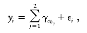where c_hij∈{1,…,C}, with c_hij representing the cluster to which haplotype h_ij belongs and with C representing the total number of clusters. If the phenotype is binary, we use the model

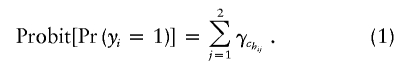Covariates can be added in the usual manner. Equation (1) assumes an additive model for the joint effect of the two haplotypes on a probit scale for a binary disease trait (corresponding approximately to a multiplicative model on an odds ratio scale, since the probit and logit links are very similar [Cox 1970]). This is done to focus the analysis on the effects of haplotype risks, but the model is easily generalized to allow for dominance if the focus is instead on genotype risks. For a dominant model, for example, one might choose instead Probit[Pr(y_i=1)]=max{γ_hchi1,γ_hchi2}.

We model the risk for haplotype cluster c as γ_c∼N(α,σ²_γ). Informative priors can be placed on α and σ²_γ; however, for all analysis performed in the present study, we fix α=0 and σ²_γ=1. This has the effect of placing an uninformative prior on the probit probabilities of p_i=Pr(y_i=1)∼Unif(0,1), which we feel is appropriate for case-control data. For data in which we have just one haplotype per phenotype, as in the data sets used for illustration in the present article, we include only a single term in the summation. Therefore, we rewrite model (1) as

where γ_chi∼N(0,1). Equation (2) should be thought of as a model for the probability that each haplotype carries a disease-susceptibility allele.

Voronoi Tessellation Structure

We cluster haplotype risks by first stochastically assigning a “center” (i.e., a haplotype), t_c∈𝒯, to each cluster c, where 𝒯=(t₁,…,t_C) denotes the current configuration of C centers. The centers may be thought of as the ancestral haplotypes from which the members of each cluster are derived. Cluster center haplotypes are free to take unobserved values. For data in which the number of markers is very large, we suggest restricting centers to the space of observed haplotypes, to improve mixing. We have implemented such an algorithm, and results are very similar to the version of the algorithm we use for all analyses in this paper, in which centers can be unobserved haplotypes (authors' unpublished data).

Having assigned a center haplotype to each cluster, we then deterministically assign each sample haplotype to the cluster with the closest center, where distance is determined by a similarity metric (see below). If a haplotype is equidistant from several centers, it is assigned to the center that appears first in the list of centers, as was done by Knorr-Held and Rasser (2000). To assist efficient mixing, the algorithm also includes a transition that shuffles the order in which the clusters are listed.

A haplotype region, R_c, is defined as

where ∥…∥ indicates “distance” in some metric space, as discussed below. Here ℋ denotes the set of unique haplotypes in the data set. Thus, R_c contains the set of observed haplotypes that are more similar to the haplotype at the center of cluster c than to any other cluster center. This partition structure is known as a “Voronoi tessellation” (Voronoi 1908) and represents the basic mechanism that we use to place haplotypes into clusters. We explore the space of possible centers, using standard Metropolis-Hastings techniques (Metropolis et al. 1953; Hastings 1970).

Similarity Metric and Gene Mapping

The effectiveness of our methodology depends upon the manner in which we determine the closeness of a sample haplotype to a particular center haplotype. We express closeness in terms of similarity (which can be thought of as inversely proportional to distance), so that the region R_c defined in equation (3) is the set of all haplotypes h that are more similar to t_c than to any other center. If we allow our similarity metric to depend upon the location x_c of the putative functional mutation for cluster c, we can use our methodology to perform gene mapping. For convenience, we restrict the x_c to be at observed marker locations. We use the same similarity metric as has been reported elsewhere (Molitor et al. 2003), a metric in which CAR models are used to evaluate haplotype risks. We express the similarity w_htc between a haplotype h and a particular center t_c as the shared length identical by state (IBS) between the two haplotypes at x_c. Specifically, we let m_r be the location of the first marker to the right of x_c at which haplotype h and cluster center haplotype t_c are not identical. Furthermore, let m^′_r denote the location of the marker immediately to the left of m_r (i.e., the last marker at which h and t_c are identical). We define

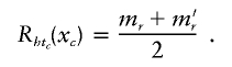We let L_htc(x_c) be the location of a similarly defined point to the left of x_c. Thus, we can write the similarity as

The similarity metric (4) can be extended in many ways. Rather than including only the region corresponding to the first difference on either side of x_c, Molitor et al. (2003) suggest a similarity metric with which one could also include regions beyond that marker. The metric is based upon the assertion that the difference was due to a mutation at the single marker locus and that the two haplotypes in question are indeed identical by descent even beyond the point of dissimilarity. In this case, one could continue to include length after a difference is encountered but assess a penalty to the shared length after such a difference. Another modification would be to define a series of probabilities at each marker location p₁,…,p_L and to use these probabilities to weight the “shared length” between markers. These probabilities might represent variation in recombination rate and would most likely be assessed by independent methods (although they could, in principle, be included in the state space and thus be estimated as part of the analysis). Thus, we might capture nonlinear patterns of linkage disequilibrium as our observations move away from the causal mutation. These probabilities could also be used as a setup for a higher level logistic or probit regression, allowing for covariates to be introduced at this stage.

Bayesian Markov Chain–Monte Carlo (MCMC) Estimation Methods

We use Gibbs sampling to obtain model parameter estimates (see, e.g., Gilks et al. 1996). This requires derivations of the full conditional distributions for each parameter—namely, the conditional distribution of each parameter, given the current estimates of all other parameters in the model. Many of the parameter updates are standard, but a few are not. We give an overview of some of the nonstandard aspects of the sampler in this section, leaving the details for appendix A.

To allow the full conditional distributions to follow standard forms, we use the convention (described by Albert and Chib [1993]) of transforming equation (2) into a normal model by introducing a latent variable y^*_i∼N(γ_chi,1). Equation (2) then becomes

where ε∼N(0,1). In each cycle of the Gibbs sampler, we generate each y^*_i, given all other parameters of the model, by simulating a normal random variable with mean γ_chij. If y_i=1, we further condition that y^*_i>0, whereas, if y_i=0, we condition that y^*_i<0. In our context, y^*_i can be interpreted as a true underlying continuous phenotype, represented by a categorical y_i=0 or 1, which serves as an imprecise indicator. Once the model has been converted to the form of equation (5), standard MCMC moves can be employed for most parameters.

To allow the number of clusters to be random instead of arbitrarily fixed ahead of time, we employ reversible jump methods (Green 1995). Instead of using the conventions common in the literature (see, e.g., Richardson and Green 1997), we employ a simpler method proposed by Denison and Holmes (2001)—a method in which, whenever the number of clusters changes, we integrate out the values of γ_c in equation (5). We define y^*=(y^*_i,…,y^*_I) and γ=(γ₁,…,γ_C), and we again let ℋ denote the space of unique haplotypes in the data set and 𝒯 denote the current set of haplotype centers. We now introduce the formula

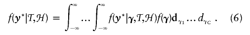When one proposes the addition of a new cluster, one would normally have to propose a new cluster risk γ_c as well. However, following Denison and Holmes (2001), we propose a new cluster based on construction of likelihoods obtained after integrating out the values of γ. At the end of each cycle of the Gibbs sampler, we then generate the current set of values for γ, using the full conditional distribution of each γ_c based on the nonintegrated likelihood, derived from equation (5). This approach is detailed and is used extensively by Denison et al. (2002). Once these parameters are updated, the values of y^*_i are updated as described above. The joint distribution of all parameters corresponding to the model formulation is

We have found that our sampler seems to mix well and to give posterior distributions that are robust to differing choices of prior for the data sets we have analyzed.

Dimensionality Issues Regarding Ambiguous Haplotypes

One appealing feature of this method is that, without changing the dimension of the parameter space, we can impute haplotypes for individuals who do not have complete haplotype information. Missing information can occur when there are missing values at some markers or when only genotype information is available. Our model does not require a risk parameter for every possible imputed haplotype. Instead, at each cycle of the Gibbs sampler, the current risk estimate for haplotype h is considered to be γ_ch. Thus, for example, one can construct a posterior distribution for the risk associated with a particular haplotype of interest. To do this, at each iteration, one simply outputs the risk parameter of the cluster to which that haplotype is assigned.

Missing information at a marker is dealt with by first selecting an incomplete haplotype and then randomly selecting one of the missing markers for imputation. We then alter the currently imputed value at the selected missing marker location to create a new haplotype that serves as our proposal haplotype. Once our proposal has been selected, we reallocate the haplotype to the cluster with the closest center and accept with a probability calculated in accordance to the Metropolis-Hastings ratio (eq. [A1]). Note that, although we must deal with individual markers in constructing our haplotype proposal, we only propose complete haplotypes in our Metropolis-Hasting ratio, thus keeping our analysis haplotype-based and never modeling markers and their associated intermarker interactions individually. Furthermore, since we do not assign a risk parameter for every possible imputed haplotype but instead infer haplotype risk indirectly, we can perform analyses in situations in which the haplotype parameter space is extremely large.

Results

In this section, we give results for analyses of real and simulated data. We used a N(0,1) prior for the values of γ and vague, “flat” priors for all other parameters. For all data sets, the sampler was run for up to 100,000 iterations for burn-in, followed by up to 5,000,000 iterations that were saved for analysis. Here we set the range of possible numbers of clusters to 1⩽C⩽25.

Choice of summary statistics to report from such analyses is not straightforward. A natural choice is to define x^max_c as the location of the functional mutation corresponding to the cluster to which most disease haplotypes are allocated at any given iteration. However, for data in which there are multiple functional mutations we often find that the posterior for x^max_c contains a single mode associated with only the most frequent of the two functional mutations. Consequently, we define a new parameter, η, which weighs the probability of a location according to risk and the number of diseased individuals associated with the location. If we assume model (2), this new parameter, η, takes on marker values, S_l, with l=1,…,L and has probability distribution function (pdf)

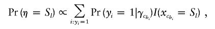where I(·) denotes an indicator function. Since we are using a probit link, we let Φ(·) denote a standard normal cumulative distribution function (cdf) and we have

Furthermore, even in the absence of phenotypes, the pattern of markers present in any given data set will result in a “null” distribution that is likely to be nonuniform for statistics of interest. For example, observed shared lengths are likely to be larger a priori in regions in which markers are less dense. To allow for this, we construct three posterior distributions when analyzing a given data set. First, we compute a null distribution for η by analyzing the data without phenotype information. (In particular, we remove the phenotype information and allow the algorithm to impute phenotypes in a manner analogous to that with which it imputes missing markers.) Second, we construct the posterior distribution for η by analyzing the data complete with phenotype information. Finally, we construct a histogram of “Bayes factors” (Kass and Raftery 1995) for η, computed by taking the ratio of posterior and null distributions at each possible η value.

Simulated Data Sets

We assess the performance of our model by using simulated haploid data. These simulations represent “proof of principle” results rather than realistic simulations of actual data sets. We simulated using a coalescent model. The coalescent was introduced by Kingman (1982) and was generalized to include recombination by Hudson (1983). Griffiths and Marjoram (1997) formalized the latter as the Ancestral Recombination Graph, which provides the formal framework for the genealogy of samples under recombination. Accessible reviews of the coalescent can be found in the work of Hudson (1991), Tavaré (1984), and Nordborg (2001). As is common in the literature, we begin by assuming a single functional mutation. We then extend this to a scenario in which there are two functional mutations. We simulate haplotypes from a single, unstructured population of fixed size, in which there is no selection acting on the region of interest. The ARG is driven by two compound parameters ν=4Nu and ρ=4Nr, where N is the (effective) haploid population size, u is the mutation probability per haplotype per generation, and r is the recombination probability per haplotype per generation (see Hudson [1991]). The computational issues involved with simulating data with high population sizes (as in our case-control simulations) combined with high recombination rates are particularly nontrivial. This is further complicated by the fact that we generate data via a rejection method that itself has low acceptance rates. Thus, because of computational limitations, we restrict ourselves to simulations with ρ=η=50, corresponding to a region on the order of 50 kb (Nordborg and Tavaré 2002) and a population size of 5,000 (in the case-control simulations).

A Single Functional Mutation

We begin by simulating data for which there is a single functional mutation. For the sake of simplicity, we assume a binary disease phenotype and haploid individuals. Let n denote the size of the sample we wish to generate and let d⩽n denote the number of diseased haploids in that sample. Assume that phenotypes are the result of a single mutation that has occurred only once and is located at x. If we assume full penetrance, the presence of d diseased haploids enforces a restriction on the space of possible genealogies underlying the data at x: the d haploids carrying the mutation must share a common ancestor among themselves before sharing a common ancestor with any of the other haplotypes. Griffiths and Tavaré (1998) and Wiuf and Donnelly (1999) provide a formal framework for this intuition in settings in which there is no recombination. However, although this constraint is enforced at x, in the presence of recombination, it will break down as we move along the haplotype away from x. Consequently, we choose to generate data using a rejection algorithm. (See, e.g., Tavaré et al. [1997] and Weiss and von Haeseler [1998] for related applications of rejection methods in a population-genetics context.) To generate samples with disease frequency close to f=d/n, we proceed as follows:

• 1. Generate the ARG for a sample of n haplotypes.
• 2. Assign a type to the most recent common ancestor of the graph and add mutations to the rest of the graph according to a Poisson process of rate ν/2.
• 3. Choose a mutation, m, uniformly at random from those present in the sample. m is our putative disease mutation.
• 4. Calculate the frequency of disease haplotypes in the sample, f^′=d^′/n, using an appropriate penetrance function π (where π is assumed to depend only on the type at m).
• 5. If ∣f^′-f∣<ε for some value of ε, output this sample, along with the generated phenotypes, with m labeled as the disease mutation.
• 6. Return to 1.

This procedure produces a set of samples along with associated phenotypes, conditioned on there being a disease phenotype of frequency close to f, the degree of closeness depending upon choice of ε (which also effects the efficiency of the algorithm). The method generalizes in a natural way to include more-complex penetrance functions and, as we indicate in the next section, more than one functional mutation.

We denote the region by the unit interval [0,1] and indicate, in figures 1–5, the true location of the functional mutation with a dashed, vertical line. In all analyses in this and subsequent sections, we remove the functional mutation(s) from the data before analysis. For all simulated data, we present the histogram of Bayes factors for η. In most of the figures, the Bayes factors are cut off at 25, so that one extremely large value cannot dominate the graph, making it impossible to see other peaks. Figure 1 shows results for 20 such analyses with f=0.25 and n=200.

Figure 1.

Histogram of Bayes factors for η as a function of mutation location in 20 simulated data sets, with one functional mutation of full penetrance and no phenocopies. Dashed vertical lines indicate “true” locations of disease-causing variants. Bayes factors >25 are truncated.

Two Functional Mutations

To produce samples in which there are two functional mutations we use the procedure given above, with n=200, but we replace step 3 with “Sample two mutations, uniformly at random from those on the graph.” We now use a penetrance function that depends upon both of the chosen mutations and accept data sets for which the disease has the target frequency. The overall disease frequency is assumed to be f=0.25. To ensure that it is reasonable to hope to find a signal associated with both mutations, we further condition on the frequencies of the two mutations chosen. To be specific, we reject the data set unless both mutations have frequency >0.1.

In figure 2, we present representative results from the analysis of 20 such data sets. Haplotypes that carry at least one of the functional mutations are labeled as diseased, with probability 0.5. All haplotypes with neither functional mutation are nondiseased.

Figure 2.

Histogram of Bayes factors for η as a function of mutation location in 20 simulated data sets, with two functional mutations and no phenocopies. Haplotypes are diseased with probability 0.5 if and only if they carry either of the functional mutations, 0 otherwise. Dashed, vertical lines indicate “true” locations of disease-causing variants. Bayes factors >25 are truncated.

We stress that these examples are designed to be illustrative of the concepts involved rather than realistic. In an attempt to consider a slightly more realistic scenario we now simulate data that can be thought of as a loose approximation to that which results from a case-control study. In particular, we generate data for a population of size n=5,000 using the preceding algorithm. We then randomly subsample 100 cases and 100 controls. These 200 haplotypes are then analyzed using our approach. We show two scenarios. In figure 3, we present representative results for a scenario in which there is a single functional mutation, located close to 0.5 and with 50% penetrance, leading to a disease with a population frequency of 5%-10%. In figure 4, we show results for a scenario in which there are two functional mutations, in which haplotypes are diseased if they carry either functional mutation and for which the disease frequency is ∼20%. The algorithm performs slightly less well in these scenarios, affected by both the case-control subsampling and the lower frequency of disease. As disease frequency is reduced, disease haplotypes tend to become more similar, and our ability to fine map over the short distances simulated here is lessened.

Figure 3.

Histogram of Bayes factors for η for in 8 simulated case-control data sets, with one functional mutation of 50% penetrance and no phenocopies. Dashed, vertical lines indicate “true” locations of disease-causing variants. Bayes factors >25 are truncated.

Figure 4.

Histogram of Bayes factors for η for in 8 simulated case-control data sets, with two functional mutations and no phenocopies. Haplotypes are diseased with probability 1 if and only if they contain either functional mutation. Dashed, vertical lines indicate “true” locations of disease causing variants. Bayes factors greater than 25 are truncated.

Cystic Fibrosis Data

This well-known data set first appeared in Kerem et al. (1989) and was recently explored in Liu et al. (2001) and Molitor et al. (2003). The data set contains 92 control and 94 disease haplotypes with each haplotype consisting of 23 RFLP markers. If we arbitrarily set the location of the first marker to be 0, the marker locations range from 0.0 to 1.7298 cM. It is known that one founder mutation, ΔF₅₀₈, falls between markers 17 and 18 and is located ∼0.88 cM away from the leftmost marker. This mutation accounts for ∼67% of disease chromosomes. This data set contains missing data, so we must impute the values at the missing markers in the manner previously described.

The posterior distributions related to η are displayed in figure 5. The posterior mode for the Bayes factor distribution was at 0.8698, for which the Bayes factor was 8.25. Histograms depicting the number of clusters that were utilized throughout the course of the MCMC simulation procedure are depicted in figure 6. Since we are clustering haplotypes associated with both healthy and disease haploids, we expect that the number of clusters selected will be more than they would if we were examining only haplotypes associated with disease. The posterior mode for the number of clusters chosen is 12 for the whole data set, whereas the posterior mode for the number of clusters associated with positive risk is only 5. Many authors have analyzed this data set (McPeek and Strahs 1999; Morris et al. 2000; Morris et al. 2002; Liu et al. 2001; Molitor et al. 2003), obtaining point estimates between 0.8 and 0.95.

Figure 5.

Histograms from the analysis of the cystic fibrosis data. a, Null for η as a function of mutation location. b, Posterior for η. c, Bayes factors for η. Dashed, vertical line indicates approximate location of ΔF₅₀₈ mutation.

Figure 6.

Histograms from the analysis of the cystic fibrosis data. Posterior distribution for (a) the total number of clusters and (b) the number of clusters associated with positive values of γ_c.

Figure 7 displays posterior mean risks (in terms of Pr(y_i=1)=Φ(γ_ci)) for each haplotype in the cystic fibrosis sample. As a by-product of our methodology, we can construct a measure of genetic heterogeneity between haplotypes. To do this, we construct an estimate of similarity between a pair of haplotypes by recording the number of times the sampler places the two haplotypes into the same cluster. We then apply agglomerative hierarchical clustering to construct a dendrogram of haplotypes shown in figure 7. Most of the haplotypes known to contain the ΔF₅₀₈ mutation are clustered together in the leftmost clade, along with eight non-ΔF₅₀₈ case haplotypes. A somewhat similar situation was encountered by Morris et al. (2002), who also performed hierarchical clustering and found a small number of non-ΔF₅₀₈ contained in a large cluster of haplotypes containing the ΔF₅₀₈ mutation and suggested that mutations borne by these non-ΔF₅₀₈ haplotypes have occurred on a background marker haplotype similar to that for the ΔF₅₀₈.

Figure 7.

Dendrogram reflecting genetic heterogeneity of cystic fibrosis haplotypes. a, Hierarchical agglomerative clustering of haplotypes, based on a similarity measure defined by the number of times each pair of haplotypes was assigned to the same cluster. b, Posterior mean estimates of Pr(y_i=1)=Φ(γ_ci) (where Φ(·) denotes a standard normal cdf) for haplotype h, arranged in the sequence given in panel a. The darkest bars indicate haplotypes known to contain the ΔF₅₀₈ mutation, the lighter bars indicate case haplotypes, and the lightest bars indicate control haplotypes.

Data for Friedrich Ataxia

Thus far, we have assumed that we have biallelic (e.g., SNP) data. Although SNP data are easy to obtain, more power might be gained by also including loci at which multiple alleles are present (for example, microsatellite loci). Our method generalizes naturally to include such a scenario. We enlarge the state space to explore the space of observed alleles at each (non-SNP) locus. Furthermore, we consider markers to be IBS at a given marker if and only if they have the same allele at that location. In the longer term, one might develop a more sophisticated similarity measure to better exploit the nature of such data, but it is of some interest to see how well our existing methodology embraces data of this more complex sort.

To illustrate this, we consider a Friedrich ataxia data set analyzed by Liu et al. (2001). The data consists of 58 disease haplotypes and 69 control haplotypes; we omitted a pair of unphased disease chromosomes. There are 12 microsatellite markers, covering a region of 15 cM. For details, see Liu et al. (2001). Results are given in figure 8. Our method preferred marker 3—located at 0.095, with a Bayes factor of 2.95—followed by marker 4, located at 0.09625 with a Bayes factor of 2.14; the true location was (0.0975, 0.0988). We note that the Bayes factors are considerably lower than for the cystic fibrosis data.

Figure 8.

Histograms of Bayes factors for values of η as a function of mutation location for Friedrich ataxia data. Dashed vertical lines indicate markers that flank the true value of mutation location.

Discussion

We have introduced a methodology for mapping based on ideas drawn from spatial statistics. We have illustrated this with analyses of both real and simulated data. We believe our methodology appears sufficiently promising to warrant further development. Also, the sampler runs quite quickly, as our C++ implementation takes ∼2.5 seconds per 1,000 iterations when analyzing the cystic fibrosis data on a 2.66 GHz Intel Xeon computer running Red Hat Linux 9.0. The program can be obtained by e-mail from J.M. (jmolitor@usc.edu). We now indicate some of the limitations of our approach and discuss obvious generalizations and other issues.

We have discussed data for which we have a binary phenotype. However, our model is, in essence, a continuous model, which we adapt for binary data by including a probit step. Thus, our methodology will deal with a continuous phenotype (by omitting the probit step). More significantly, we assume haploid individuals. Diploid data with known haplotypes fits within our framework via the inclusion of both haplotypes and, if desired, interaction terms for pairs of clusters. However, if we have genotype data and haplotypes are unknown, a more substantial adaptation is required. Essentially, we propose the addition of a further layer to the model in which genotypes are assigned to haplotypes before these haplotypes are then assigned to their ancestral clusters. This layer will be explored as part of the same MCMC model, thus integrating the analysis of the haplotypes with the assignment of genotypes to haplotypes. We propose to develop these ideas, including more complex situations such as pedigree-based analyses, in a subsequent paper.

We currently assign haplotypes to centers in a conditionally deterministic fashion. In other words, if one knows the centers and the similarity metric parameters, then one can assign haplotypes to clusters with certainty. Over the course of iterations, the centers and the values of x_c change, so a probabilistic distribution of cluster assignments for each haplotype is effectively generated. However, it might be desirable to make probabilistic assignments at each iteration. If the similarity between haplotype h and a certain cluster center c^′ is w_h,c^′, then the haplotype could be assigned to cluster c^′ with probability

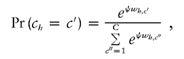where ψ is a smoothing parameter to be estimated. As ψ increases, the chance that we will choose the cluster with the most similar center increases. Note that, if ψ=0, cluster allocation is uniformly random, completely ignoring the similarity, and, as ψ→∞, each haplotype is assigned with certainty to the most similar center, bringing us back to our original Voronoi-based method. This probabilistic approach is close in spirit to the commonly used Potts model (see Green and Richardson 2002).

Like our proposed approach, the method of Molitor et al. (2003) used techniques based in spatial analysis. They used CAR techniques (Cressie 1993) that include just one parameter for the location of a disease-causing mutation and therefore had limited ability to detect multiple disease mutations. Also, the CAR approach requires a risk parameter for each haplotype and therefore does not scale well when there is a large number of haplotypes. This is especially true when there are missing marker values, as one needs a separate risk parameter not only for every observed haplotype but also for every haplotype that can arise as a result of missing value imputation. One of the strengths of our method is the way it places haplotypes into clusters, thereby potentially allowing for detection of multiple disease-causing variants. The clustering approach is close in spirit to the coalescent, allowing our clusters to be interpreted as the set of descendants of common ancestral haplotypes.

Appendix A : MCMC Algorithm

Reversible Jump MCMC

We make the prior assumption that all haplotype center configurations are equally likely and that the number of clusters C is constrained to lie within [C_min,C_max]. By using an uninformative prior structure on the number of centers and by proposing and deleting centers with equal probability, we effectively cancel out our center proposal and prior distributions when Metropolis-Hastings updates are made (see Denison et al. 2002, p. 53). Using equation (6), we can propose a new cluster (Birth Move) by proposing a new center and labeling the set of center values with the new addition as 𝒯^new while the current set is denoted as 𝒯^old. We then use the following Metropolis-Hastings ratio to decide whether to accept the proposal:

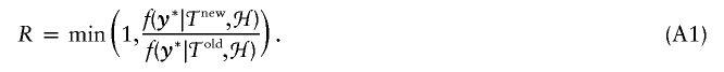We propose a new center by randomly generating a new haplotype. Note that, since we are dealing with a discrete set of centers instead of continuous variables, no Jacobian term is required in equation (A1). Cluster deletions are accomplished by randomly selecting one of the existing clusters and removing it. We also propose new states in which one of the existing clusters is chosen at random and its center haplotype is changed to a new type. Whenever we propose a new center configuration 𝒯^new, a new set of allocations of haplotypes to clusters must be deterministically calculated.

Updates That Do Not Affect Cluster Allocation

The updates of y^*_i and γ_c do not have a direct impact on how haplotypes are allocated to clusters. Each parameter is updated from its full conditional distribution according to equation (5), using standard normal theory (see, e.g., Carlin and Louis 2000).

Updates Affecting Cluster Allocation

The following parameter proposals have a direct impact on how haplotypes are allocated to clusters and therefore require that haplotypes be reallocated to clusters after each successful proposal. First, we define z_i=y^*_i and define an I×C matrix X, which has elements X_ij=1 if c_hi=j and 0 otherwise. We then rewrite equation (5) as

If we assume a prior γ∼N(μ,Σ), then f(γ|z)∼N(μ^*,Σ^*) with

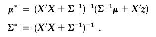Parameter proposals are evaluated by constructing a Metropolis-Hastings ratio made from the following marginal likelihood.

where

Here, our prior for γ is γ∼N(0,I).

We choose uniformly at random from the following five updates. Each update is consists of a proposal that is accepted according to a standard Metropolis-Hastings ratio based on equation (6).

• 1. Update x_c

  We sample the location of the functional mutation x_c using a nonstandard method. With probability 0.75, we propose a new value of x_c based on a random perturbation of the current value, namely x^new_c=x^old_c+Δ, where Δ can be tuned during the burn-in phase of the sampler. We have found that the value of x_c can often mix poorly, so, with probability 0.25, we select x^new_c randomly from all available marker locations. In either case, x^new_c changes the set of similarities of haplotypes to cluster c. The acceptance probability of x^new_c is calculated by reallocating haplotypes to centers by use of the new similarities and then calculating a standard Metropolis-Hastings ratio. When this method is used, x_c generally moves freely during the early burn-in phase of the sampler and then settles down to a relatively narrow region as the sampler progresses.

• 2. Cluster Birth Move

  A new center is proposed by randomly selecting a haplotype that is not already a center and randomly selecting an x_c from all possible marker values.

• 3. Cluster Death Move

  We randomly select a center haplotype and its associated x_c from the current set of center haplotypes and delete it.

• 4. Cluster Center Move

  One of the existing center haplotypes is randomly selected and is changed to a haplotype that is not already a center haplotype. The new center configuration, 𝒯^new, contains the same number of haplotype centers as before, but with one center altered.

  We alter a center haplotype by selecting a percentage of markers and then replacing each allele at each chosen marker with an allele randomly selected from all alleles observed in the data set at that marker. The percentage of markers chosen is a tuning parameter that is modified during the burn-in phase of the sampler. However, to improve mixing, we construct a center proposal 25% of the time, by randomly choosing a center haplotype from the entire space of possible haplotypes that are not currently centers, in a manner similar to how the values of x_c are updated.

• 5. Shuffle Move

  The order of the clusters is randomly permuted.

References

- Albert JH, Chib S (1993) Bayesian analysis of binary and polychotomous response data. J Am Stat Assoc 88:669–679 [Google Scholar]
- Carlin BP, Louis TA (2000) Bayes and empirical Bayes methods for data analysis, second editon. Chapman & Hall/CRC, Boca Raton, FL [Google Scholar]
- Cox DR (1970) Analysis of binary data. Chapman and Hall, London [Google Scholar]
- Cressie NAC (1993) Statistics for spatial data, revised edition. John Wiley & Sons, New York [Google Scholar]
- Denison D, Holmes C (2001) Bayesian partitioning for estimating disease risk. Biometrics 57:143–149 [DOI] [PubMed] [Google Scholar]
- Denison DGT, Holmes CC, Mallick BK, Smith AFM (2002) Bayesian methods for nonlinear classification and regression. John Wiley & Sons, New York [Google Scholar]
- Gilks WR, Richardson S, Spiegelhalter DJ (eds) (1996) Markov Chain Monte Carlo in practice. Chapman and Hall, London [Google Scholar]
- Green P (1995) Reversible jump Markov chain Monte Carlo computation and Bayesian model determination. Biometrika 82:711–732 [Google Scholar]
- Green P, Richardson S (2002) Hidden Markov models and disease mapping. J Am Stat Assoc 97:1055–1070 [Google Scholar]
- Griffiths RC, Marjoram P (1997) An ancestral recombination graph. In: Donnelly P, Tavaré S (eds) Progress in population genetics and human evolution. Springer Verlag, New York, pp 100–117 [Google Scholar]
- Griffiths RC, Tavaré S (1998) The age of a mutation in a general coalescent tree. Stochastic Models 14:273–295 [Google Scholar]
- Hastings WK (1970) Monte Carlo sampling methods using Markov chains and their applications. Biometrika 57:97–109 [Google Scholar]
- Hudson RR (1983) Properties of a neutral allele model with intragenic recombination. Theor Popul Biol 23:183–201 [DOI] [PubMed] [Google Scholar]
- Hudson RR (1991) Gene genealogies and the coalescent process. In: Futuyma D, Antonovics J (eds) Oxford surveys in evolutionary biology, volume 7. Oxford University Press, Oxford, pp 1–44 [Google Scholar]
- Kass R, Raftery A (1995) Bayes factors. J Am Stat Assoc 90:773–795 [Google Scholar]
- Kerem B, Rommens JM, Buchanan JA, Markiewicz D, Cox TK, Chakravarti A, Buchwald M, Tsui LC (1989) Identification of the cystic fibrosis gene: genetic analysis. Science 245:1073–1080 [DOI] [PubMed] [Google Scholar]
- Kingman JFC (1982) On the genealogy of large populations. J Appl Probab 19A:27–43 [Google Scholar]
- Knorr-Held B, Rasser L (2000) Bayesian detection of clusters and discontinuities in disease maps. Biometrics 56:13–21 [DOI] [PubMed] [Google Scholar]
- Liu JS, Sabatti C, Teng J, Keats BJB, Risch N (2001) Bayesian analysis of haplotypes for linkage disequilibrium mapping. Genome Res 11:1716–1724 10.1101/gr.194801 [DOI] [PMC free article] [PubMed] [Google Scholar]
- McPeek MS, Strahs A (1999) Assessment of linkage disequilibrium by the decay of haplotype sharing, with application to fine-scale genetic mapping. Am J Hum Genet 65:858–875 10.1086/302537 [DOI] [PMC free article] [PubMed] [Google Scholar]
- Metropolis N, Rosenbluth AW, Rosenbluth MN, Teller AH, Teller E (1953) Equations of state calculations by fast computing machines. J Chem Phys 21:1087–1091 [Google Scholar]
- Molitor J, Marjoram P, Thomas DC (2003) Application of Bayesian spatial statistical methods to the analysis of haplotypes effects and gene mapping. Genet Epidemiol 25:95–105 10.1002/gepi.10251 [DOI] [PubMed] [Google Scholar]
- Morris AP, Whittaker JC, Balding DJ (2000) Bayesian fine-scale mapping of disease loci, by hidden Markov models. Am J Hum Genet 67:155–169 10.1086/302956 [DOI] [PMC free article] [PubMed] [Google Scholar]
- Morris AP, Whittaker JC, Balding DJ (2002) Fine-scale mapping of disease loci via shattered coalescent modeling of genealogies. Am J Hum Genet 70:686–707 10.1086/339271 [DOI] [PMC free article] [PubMed] [Google Scholar]
- Nordborg M (2001) Coalescent theory. In: Balding DJ, Bishop MJ, Cannings C (eds) Handbook of statistical genetics. John Wiley & Sons, New York, pp 179–208 [Google Scholar]
- Nordborg N, Tavaré S (2002) Linkage disequilibrium: what history has to tell us. Trends Genet 18:83–90 10.1016/S0168-9525(02)02557-X [DOI] [PubMed] [Google Scholar]
- Okabe A, Boots B, Sugihara K (1992) Spatial tesselations: concepts and applications of Voronoi diagrams. John Wiley & Sons, New York [Google Scholar]
- Richardson S, Green P (1997) On Bayesian analysis of mixtures with an unknown number of components. J Roy Stat Soc B 59:731–792 10.1111/1467-9868.00095 [DOI] [Google Scholar]
- Tavaré S (1984) Line-of-descent and genealogical processes, and their applications in population genetics models. Theor Popul Biol 26:119–164 [DOI] [PubMed] [Google Scholar]
- Tavaré S, Balding DJ, Griffiths RC, Donnelly P (1997) Inferring coalescence times for molecular sequence data. Genetics 145:505–518 [DOI] [PMC free article] [PubMed] [Google Scholar]
- Thomas DC, Morrison J, Clayton DG (2001) Bayes estimates of haplotype effects. Genet Epidemiol 21:S712–S717 [DOI] [PubMed] [Google Scholar]
- Voronoi MG (1908) Nouvelles applications des paramètres continus à la théorie des formes quadratiques. J Reine Angew Math 134:198–287 [Google Scholar]
- Weiss G, von Haeseler A (1998) Inference of population history using a likelihood approach. Genetics 149:1539–1546 [DOI] [PMC free article] [PubMed] [Google Scholar]
- Wiuf C, Donnelly P (1999) Conditional genealogies and the age of a neutral mutant. Theor Popul Biol 56:183–201 10.1006/tpbi.1998.1411 [DOI] [PubMed] [Google Scholar]