Genome Scan Meta-Analysis of Schizophrenia and Bipolar Disorder, Part I: Methods and Power Analysis

Abstract

This is the first of three articles on a meta-analysis of genome scans of schizophrenia (SCZ) and bipolar disorder (BPD) that uses the rank-based genome scan meta-analysis (GSMA) method. Here we used simulation to determine the power of GSMA to detect linkage and to identify thresholds of significance. We simulated replicates resembling the SCZ data set (20 scans; 1,208 pedigrees) and two BPD data sets using very narrow (9 scans; 347 pedigrees) and narrow (14 scans; 512 pedigrees) diagnoses. Samples were approximated by sets of affected sibling pairs with incomplete parental data. Genotypes were simulated and nonparametric linkage (NPL) scores computed for 20 180-cM chromosomes, each containing six 30-cM bins, with three markers/bin (or two, for some scans). Genomes contained 0, 1, 5, or 10 linked loci, and we assumed relative risk to siblings (λ_sibs) values of 1.15, 1.2, 1.3, or 1.4. For each replicate, bins were ranked within-study by maximum NPL scores, and the ranks were averaged (R_avg) across scans. Analyses were repeated with weighted ranks ( for each scan). Two P values were determined for each R_avg: P_AvgRnk (the pointwise probability) and P_ord (the probability, given the bin’s place in the order of average ranks). GSMA detected linkage with power comparable to or greater than the underlying NPL scores. Weighting for sample size increased power. When no genomewide significant P values were observed, the presence of linkage could be inferred from the number of bins with nominally significant P_AvgRnk, P_ord, or (most powerfully) both. The results suggest that GSMA can detect linkage across multiple genome scans.

Introduction

Schizophrenia (SCZ; locus SCZD [MIM #181500]) and bipolar disorder (BPD; loci MAFD1 [MIM 125480] and MAFD2 [MIM 309200]) are severe, common, genetically complex psychiatric phenotypes. As discussed in parts II and III of this series, there have been at least 20 SCZ and 22 BPD genome scans to date, with others in progress. Most twin and family studies suggest that there are independent genetic factors underlying these disorders (Levinson and Mowry 2000), but overlapping factors remain a possibility (Berrettini 2000): severe BPD cases have symptoms resembling SCZ, “schizoaffective” cases with mixed symptoms have increased familial risks of both disorders, and there are chromosomal regions in which linkage evidence has been reported for both SCZ and BPD. Most of the available genome scan studies were initiated early in the 1990s and have been relatively small; for SCZ, the average study included ∼60 pedigrees, and for BPD the average study included 28. There have been only one BPD and three SCZ studies reported with >100 pedigrees in the complete scan, although a number of larger studies are currently in progress.

Although statistically significant findings have been reported, and some of these have been supported by other studies, there is no locus, for either disorder, that has consistently produced evidence for linkage in most studies. It is, therefore, likely that susceptibility is conferred by DNA sequence variations at combinations of loci, each with a small effect on risk (common polygenes), that the loci of greatest effect vary considerably across families and samples (locus heterogeneity), or both. It may be necessary to combine the results of multiple studies to have adequate power to detect these loci, until much larger samples are available.

The present series of articles uses a rank-based method, genome scan meta-analysis (GSMA) (Wise et al. 1999), to evaluate the evidence for linkage across available SCZ and BPD genome scans. This first article briefly reviews the theoretical basis for the method and then describes a set of simulation studies that estimate the power of GSMA to detect linked loci in data sets comparable to the SCZ and BPD data sets, across a range of genetic models, providing empirical standards for assessing statistical significance. The second and third articles then describe the GSMAs of SCZ and BPD, respectively (Lewis et al. 2003 [in this issue]; Segurado et al. 2003 [in this issue]).

Several other strategies are available for meta-analysis of linkage data. The most robust approach would be to obtain the original genotypes for each study, construct a combined map of the markers, and perform new linkage analyses. However, the genotypes are not available for all SCZ and BPD studies and in some cases are restricted by industry relationships. Construction of a combined map has also been problematic, although the new deCode map (Kong et al. 2002) should make this easier in the future. An alternative approach, multiple scan probability (MSP) (Badner and Gershon 2002b), has been applied to published SCZ and BPD data (Badner and Gershon 2002a). This approach combines P values after correcting for the size of the linkage area. GSMA and MSP are compared further below.

GSMA has a number of advantages over other available methods. It requires only placing markers within 30-cM bins, rather than determining precise positional relationships (although precision in localizing the linkage signal is thereby reduced). Because raw data are not required, it is straightforward for investigators to provide the necessary results (linkage scores, P values, or ranked data) for each location. When several genetic analyses have been performed in a particular study, results can be maximized to produce a single set of ranks for that study. No assumptions are made about models of inheritance or of genetic heterogeneity. However, GSMA provides no formal test of genetic hetereogeneity, and interpretation of genomewide statistical significance currently relies on empirical grounds.

In contrast to the GSMA, meta-analysis in epidemiological studies provides a combined effect size (e.g., relative risk) with its confidence interval. These methods have directly interpretable parameter values and allow testing of heterogeneity between studies, but they require each included study to use the same statistical analysis and to test the same hypothesis. Such methods are difficult to apply to linkage studies, which commonly report a LOD score (i.e., a measure of significance) and not an effect size. Their extension to assess evidence of linkage across a region is also not straightforward. Novel methods for meta-analysis of linkage studies are therefore needed.

In summary, on the basis of the empirical standards for assessing significance reported in this article, the GSMA of SCZ genome scans produced significant evidence for linkage for 12–19 of 120 bins, depending on the approach to assessing significance. By contrast, the GSMA of BPD scans produced no clear statistically significant evidence for linkage, and the analysis was complicated by the many combinations of diagnoses included in linkage analyses by different studies. The bins with nominally significant P values for BPD showed no clear overlap with the most significant bins for SCZ. Results for each disorder and their implications are discussed in the second and third articles in this series (Lewis et al. 2003 [in this issue]; Segurado et al. 2003 [in this issue]).

Rationale for the Simulation Studies

The simulation studies were intended to clarify the kinds of genetic effects that might be detected by GSMA in the SCZ and BPD data sets. Simplifying assumptions were necessary, given the unlimited range of possible genetic models. GSMA should have the greatest power to detect effects that are present in a substantial number of the individual studies (common polygenes) and less power to detect effects that are present in very few families or samples (extreme locus heterogeneity). We therefore designed a set of simulation studies based on the common polygene model. We recognize that there could be susceptibility loci for SCZ and/or BPD that can be detected only in particular ethnic groups or pedigree structures. As in all studies of complex disorders, GSMA can only produce positive evidence for certain effects; it cannot exclude other hypotheses.

There are advantages to using simulated samples of affected sibling pairs (ASPs) to model common polygenes. For families containing a single ASP, if one ignores diagnoses in parents or other relatives and if transmission is not recessive (i.e., if risks are similar in sibs, parents, and offspring), then there is a straightforward relationship between the locus-specific relative risk to siblings of affected probands (λ_sibs) and the power to detect linkage for either a single major locus or a multiplicative interaction among loci (James 1971; Risch 1987, 1990). Studying samples of ASPs therefore simplifies the simulations, because the exact choice of parameter values becomes unimportant as long as they predict the desired locus-specific λ_sibs (although, in the real case, λ_sibs values can be distorted by imprecise estimates of population prevalence, particularly for rarer disorders). A disadvantage of this approach is that extended pedigrees could have greater power under certain genetic models, but it would have been difficult here to select a limited yet plausible range of models. Much of the linkage information in available SCZ and BPD samples is contained in small nuclear families and, thus, in the sharing of alleles by ASPs. Therefore, we decided to assess the power of GSMA in samples of families with two affected sibs each (independent ASPs). Only dominant transmission models were studied, because recessive inheritance is unlikely, given the absence of differences between risks to sibs versus risks to parents/offspring for either disorder (Risch 1990) and because ASPs have less power to detect linkage under dominant transmission and, thus, results should be conservative. For comparison, recessive inheritance has been studied for one of the models at the lowest value of λ_sibs (1.15), and power was indeed substantially greater than for dominant transmission.

There is a common misconception that ASP analyses cannot detect linkage in the presence of genetic heterogeneity. For a known risk allele, locus-specific λ_sibs could be computed by genotyping a population-based sample to establish the risk allele frequency and penetrances and then determining the relative risk to a carrier probands’ sibs, parents, and offspring versus the population risk. In the absence of recessive effects, risks to siblings, parents, and offspring will be similar, and, in families transmitting the risk allele, ASP identical-by-descent (IBD) allele sharing would be predicted by the locus-specific λ_sibs: the proportion of ASPs sharing 0 alleles IBD, z₀, is 0.25/λ_sibs (Risch 1990). However, in linkage studies, the risk locus is unknown, and sharing is measured at nearby marker loci. If 20% of probands carry an allele that increases risk to sibs by threefold, the observed marker z₀ will be the weighted average of z₀ in the 80% families with no linkage (0.25) and in the 20% families with linkage (0.25/3=0.0833); thus, populationwide z₀=0.21667, and power will be similar to that for a locus-specific λ_sibs=0.25/0.21667=1.1538. Power will be similarly reduced for nonparametric analyses and for parametric heterogeneity LOD score analyses. Thus, in the studies presented here, genetic effects are expressed as populationwide λ_sibs. Results would be similar regardless of whether each locus produced a smaller increase in risk in many families or a larger increase in a small proportion of families.

We therefore estimated, for each actual SCZ or BPD genome scan, the number of ASPs with roughly equivalent linkage information, as described below. Genotypes were simulated for large pools of ASP families (two parents of unknown diagnosis and two affected siblings) on the basis of genetic models predicting specific values of λ_sibs or no linkage, and appropriate types and numbers of ASPs were randomly drawn from the pools of families. Given the λ_sibs values used here (1.15–1.4), individual samples in each replicate varied greatly in IBD sharing proportions, as would be observed with either a common polygene model or a moderate locus heterogeneity model. Linkage analyses were performed using nonparametric linkage (NPL) Z_all scores (GENEHUNTER 2.0), which correlate highly with ASP analyses. NPL scores simplified the simulation procedure because, even when multipoint analyses are used (as was the case here), NPL scores maximize at marker loci rather than between loci, so that only one data point per marker had to be considered.

Material and Methods

GSMA

GSMA was developed to deal with the diverse study designs, analysis methods, and marker densities used in genome scan studies. GSMA divides the autosomes into 120 bins of ∼30 cM in length (X and Y chromosomes are not considered here). The 30-cM bin width is the largest that divides the smallest chromosomes into two bins each, and it ensures that scores within bins are correlated strongly and those between bins more weakly; for the real data sets in the following two articles (Lewis et al. 2003 [in this issue]; Segurado et al. 2003 [in this issue]), we have assessed the effects of bin placement by combining adjacent bins, but we have not comprehensively studied alternative bin widths. For consistency across GSMAs, the boundaries of these bins are defined by Généthon markers, as shown in the following two articles (Lewis et al. 2003 [in this issue]; Segurado et al. 2003 [in this issue]). Thus, markers located between ∼0 cM and 30 cM on chromosome 1 are assigned to bin 1.1, those between 30 cM and 60 cM to bin 1.2, etc. To simplify the simulation studies reported here, a 3,600-cM genome was assumed, comprised of 20 180-cM autosomes, each containing six bins.

The ranking procedure is illustrated in appendix A. In brief, for each of N studies, the bins are ranked (1 = best) on the basis of the maximum linkage score or lowest P value observed within each bin. These are within-study ranks (R_study). All negative linkage scores are considered equivalent to 0, for consistency with methods that produce no negative values—we did not study the influence of this “floor” effect on results (i.e., ignoring the degree of negativity of a score, which could counterbalance a very positive score in another study). For bins with the same maximum scores (such as those with 0 scores), each bin is assigned the mean value of the ranks in their range. For weighted analyses, each rank is multiplied by the weight for that study—here, the standardized (see below). Then, the average rank (R_avg) is computed for each bin, across all N studies. The mean is 60.5 under the null hypothesis, and values closer to 1 indicate a clustering of evidence for linkage in that bin. Theoretical thresholds of significance for unweighted analyses are shown in order to provide the reader with a sense of the relevant ranges of values for different sample sizes. (Note: previous GSMAs reported R_study values ranked in descending order and summed rather than averaged them. The two procedures are statistically identical, but it is more intuitive for 1 to be “best.”)

The assessment of statistical significance is summarized in the third table of appendix A, in table 1, and in figure 1.

Table 1.

P Values Based on Ordered Average Ranks (P_ord)

			Randomly Permuted Replicatesb
Bin	ObservedRavga	PAvgRnk	RavgReplicate1	RavgReplicate2	…	RavgReplicate5,000	Mean Ravg ± SD	Pordc
1st Place	30.3	.00006	35.8	41.1	…	36.6	39.2 ± 3.1	.0104
2nd Place	31.5	.00015	38.5	43.0	…	42.4	42.0 ± 2.3	.0002
3rd Place	34.2	.00044	40.8	43.4	…	45.0	43.6 ± 1.9	.0002
4th Place	34.3	.00045	40.9	44.0	…	45.5	44.7 ± 1.7	.0002
…	…	…	…	…	…	…	…	…
120th Place	82.2	.99	83.1	77.2		79.1	81.5 ± 3.0	1.0

^aWeighted R_avg values for one GSMA replicate (20 studies, 10 disease loci, λ_sibs=1.15; ed2md8 in table 5), sorted with the first-place (“best”) bin at the bottom of the column.

^bR_study values were randomly reassigned into columns, and R_avg was computed for each bin of each replicate and then sorted. Means and SDs describe the R_avg distributions for 1st-place, 2nd-place, etc., bins with no linkage.

^c“By chance, how frequently would the average rank for a bin in the same place be as low as or lower than the observed average rank?” P_ord=(r+1)/(n+1), where r is the number of randomly permuted replicates for which the R_avg of the jth-place bin is less than or equal to the observed jth-place R_avg, and n is the number of replicates (North et al. 2002). See figure 1 for illustration.

Figure 1.

Determining P_ord: observed and expected ordered R_avg values. The black line shows the 120 observed R_avg values, sorted with the first-place bin on the right. The light gray line and vertical error bars show the mean ± 2 SD of the jth-place bin from 5,000 random permutations. In the absence of linkage, R_avg values lower than the expected distribution are observed infrequently throughout the genome. With linkage, they are clustered among the highest values of R_avg, as shown here. As shown in table 1, P_ord is the probability of observing a given value of R_avg (black line) by chance, given its place in the order of observed R_avg values, which is determined from the distribution of ordered R_avg values (light gray line and error bars).

P_AvgRnk is the pointwise probability of observing a given R_avg for a bin by chance, in a GSMA of N studies (third table in appendix A). This can be determined theoretically (see appendix B) or by permutation: for a GSMA of N studies, for each permuted replicate, the observed 120 R_study values for each study are randomly reassigned to bins and then averaged across studies for each bin. At least 5,000 replicates are produced, or a larger number to produce stable estimates of small or marginal P values. If the observed R_avg is ⩽38.9, then P_AvgRnk is the proportion of bins in the random replicates with R_avg=38.9 (e.g., among 120 bins × 5,000 replicates).

P_ord (short for “P_AvgRnk|order”) is the probability of observing a given R_avg for a bin by chance in bins with the same “place” in the ascending order of R_avg values in randomly permuted replicates (table 1; fig. 1). Thus, in the permutation test described above, the R_avg values for each replicate are now sorted by size. If the observed fourth-best R_avg=31.0, P_ord is the probability of observing a value ⩽31.0 in the 5,000 fourth-place bins in the replicates. Consider the analogy of a race: P_AvgRnk determines which bins are the “fastest runners,” whereas P_ord determines whether it is a “fast race” (i.e., whether the top finishers all ran faster than the top finishers in most races). As shown by the simulation studies reported below, it is this aggregate information about the set of most significant bins that provides additional information about linkage when genomewide significance is not observed for P_AvgRnk.

P_AvgRnk and P_ord have been computed as (r+1)/(n+1), where r is the number of replicates exceeding a particular score and n is the total number of replicates. As explained by North et al. (2002, p. 439), “if the null hypothesis is true, then the test statistics of the n replicates and the test statistic of the actual data are all realizations of the same random variable,” and thus the P value is more accurate when the data set being tested is included in the ranking of all known outcomes. Like P_AvgRnk, P_ord is a pointwise value—∼5% of bins will have P_ord⩽.05 in unlinked replicates, although these values will be scattered throughout both large and small ranks. The 5% threshold for genomewide significance of each type of P value must therefore be corrected for 120 bins: .05/120=.000417. This is larger than the threshold of pointwise P=.00002 for linkage results (Lander and Kruglyak 1995), because, for GSMA, inference is restricted to discrete bins of 30 cM. Statistical properties of P_ord, including nonindependence of the values, are discussed further below.

The terminology described above is summarized in appendix C.

Description of the Samples

The simulated GSMA data sets were based on three of the SCZ and BPD data sets described in the second and third papers in this series, respectively.

• 1. The simulated SCZ data sets (table 2) approximated the linkage information of the 20 genome scan analyses from 17 independent projects included in the SCZ GSMA, using narrow diagnoses (usually SCZ plus schizoaffective disorders). Simulated sample sizes were the reported number of ASPs in a corresponding study or an estimate based on a multicenter SCZ sample (Levinson et al. 2000), where (N[genotypedcases]-N[informativepedigrees])≈1.39×(N[independentASPs]). The proportion of genotyped parents was as reported or was estimated from study descriptions and was increased when many unaffected relatives were genotyped. Average marker spacing was 10 or 15 cM, similar to the corresponding study.
• 2. The simulated BPD data sets resembled sets of genome scans in the BPD GSMA. These studies considered various diagnostic combinations of bipolar-I, bipolar-II, schizoaffective disorder–bipolar type, recurrent major depression, and sometimes other diagnoses. Thus, the number of affected cases and informative families varied according to the model. The simulated data sets resembled those for the two narrowest models considered in the BPD GSMA: the BP-VN (very narrow) data set (table 3) includes nine simulated samples whose sizes resemble those of the nine BPD scans analyzed under a very narrow diagnostic model, considering only BPI and SAB as affected; the BP-N (narrow) data set (table 4) includes 14 simulated samples whose sizes resemble those of the 14 BPD scans analyzed under a narrow model, considering BPI, SAB, and BPII cases as affected. Numbers of ASPs were determined as for SCZ, with zero, one, or two genotyped parents each in ∼33% of families, on the basis of the SCZ data (because pedigree structure details were sometimes unavailable). Average marker spacing was 10 cM.

Table 2.

SCZ Simulated Data Set

	Actual Study		Simulation Studya			No. of ASP Families with N Genotyped Parents
Sample	No. ofPedigrees	No. ofCases	Weight	MapDensity(cM)	No. ofASPs	N=2	N=1	N=0
1	294	669	2.3165	10	330	135	115	80
2	185	390	1.7687	10	240	85	80	75
3	71	171	1.1711	10	90	85	5	0
4	81	170	1.1677	15	90	0	0	90
5	77	179	1.1982	15	75	12	19	44
6	67	164	1.1469	15	75	12	19	44
7	74	169	1.1643	15	75	12	19	44
8	54	146	1.0822	10	55	32	19	4
9	60	132	1.0290	10	72	15	25	30
10	43	126	1.0053	10	57	30	19	8
11	53	113	.9520	10	60	10	25	25
12	43	96	.8775	10	56	15	23	18
13	30	79	.7960	10	45	4	27	14
14	22	79	.7960	10	65	20	30	15
15	21	58	.6821	10	40	32	4	4
16	13	56	.6702	10	50	20	20	10
17	1	43	.5873	10	50	5	25	20
18	5	37	.5448	10	40	15	15	10
19	9	35	.5298	10	30	15	9	6
20	5	33	.5145	10	30	16	8	6
Total	1,208	2,945	20.0000		1,625	570	506	547

^aNumbers of pedigrees and genotyped affected cases are those in the actual study (see the second article in this series [Lewis et al. 2003 {in this issue}]). Number of ASPs (simulation study) was assigned as described in the text. Weight = , where “cases” = number of genotyped affected cases in the actual study (see text).

Table 3.

BP-VN Simulated Data Set

	Actual Study		Simulation Studya		No. of ASP Families with N Genotyped Parents
Sample	No. ofPedigrees	No. ofCases	Weight	No. ofASPs	N=2	N=1	N=0
1	2	24	.527	18	6	6	6
2	7	27	.559	17	6	6	5
3	15	41	.689	22	7	7	8
4	13	40	.681	23	8	8	7
5	5	42	.698	31	10	10	11
6	41	107	1.114	55	18	18	19
7	39	115	1.155	63	21	21	21
8	97	264	1.749	139	46	46	47
9	128	288	1.827	133	44	44	45
Total	347	948	9.000	501	166	166	169

^aNumbers of pedigrees and genotyped affected cases are those in the actual study (see the third article in this series [Segurado et al. 2003 {in this issue}]). See the table 2 footnote and the text for details.

Table 4.

BP-N Simulated Data Set

	Actual Study		Simulation Studya		No. of ASP Families with N Genotyped Parents
Sample	No. ofPedigrees	No. ofCases	Weight	No. ofASPs	N=2	N=1	N=0
1	2	24	.481	18	6	6	6
2	7	39	.614	27	9	9	9
3	7	36	.589	24	8	8	8
4	15	46	.666	26	9	9	8
5	13	44	.652	26	9	9	8
6	20	48	.681	23	8	8	7
7	5	42	.637	31	10	10	11
8	22	118	1.067	80	27	27	26
9	41	107	1.016	55	18	18	19
10	39	208	1.417	141	47	47	47
11	51	128	1.112	64	21	21	22
12	65	232	1.496	139	46	46	47
13	97	336	1.801	199	66	66	67
14	128	325	1.771	164	55	55	54
Total	512	1,733	14.000	1,017	339	339	339

^aSee the table 2 footnote and the text for details.

Simulation Procedure

Genotypes were created by simulation for chromosomes with either no linked locus, or with one linked disease locus under one of four dominant genetic models:

• 1. λ_sibs=1.15 [q(D)=0.434, f(dd)=0.01, f(Dd,DD)=0.1];
• 2. λ_sibs=1.2 [q(D)=0.0169, f(dd)=0.006, f(Dd,DD)=0.03];
• 3. λ_sibs=1.3 [q(D)=0.0173, f(dd)=0.005, f(Dd,DD)=0.03];
• 4. λ_sibs=1.4 [q(D)=0.0244, f(dd)=0.004, f(Dd,DD)=0.025];

where D indicates the disease allele, d the wild-type allele, q the allele frequency, and f the penetrance. This range of values was selected because samples of 500–1,000 ASPs have been shown to have reasonable power to detect linkage at values ∼1.3–1.4, with power increasing rapidly above this range and decreasing rapidly below it (Hauser et al. 1996).

To confirm that power would be greater for recessive transmission, a single set of replicates was created for the SCZ data set as discussed below, using parameter values predicting λ_sibs=1.15 [q(D)=0.276, f(dd,Dd)=0.01, f(DD)=0.04].

LINKAGE-format files were created with sets of families with two parents of unknown diagnosis and two affected offspring. Simulated genotypes were created using GENSIM (Kruglyak et al. 1996; Kruglyak and Daly 1998). The structure of the simulated chromosomes is shown in figure 2. Each chromosome was 180 cM long (six 30-cM bins). Bins contained three markers (10-cM spacing), except for four SCZ scans with 15-cM spacing. Disease loci were conservatively placed halfway between adjacent markers, given that many other aspects of the procedure were idealized (e.g., identical marker maps in all studies, no genotyping errors).

Figure 2.

Marker maps for simulation studies. Genotypes were simulated for 180-cM chromosomes, on each of which six 30-cM bins (segments) were structured as shown. Marker locations are M1, M2, M3. For the SCZ data sets, some studies had 10-cM marker spacing (A) and others had 15-cM spacing (B); all BP data sets were simulated with 10 cM spacing. Linked (disease) and unlinked (nondisease) chromosomes were created (C). Disease loci (indicated by “D”) were located midway between two markers, either in the first (edge) or third (middle) bin. Genomes consisted of 20 chromosomes (120 bins); see table 5 for structures of genomes.

Four types of genomes were created (table 5), with 1, 5, or 10 linked loci in “edge” or “mid” bins. Lower multipoint NPL scores were anticipated near the edges of chromosomes because of reduced information content. The value of λ_sibs was constant for all disease loci in a simulated genome. Sets of “linked” chromosomes for 10,000 families were created for each of 24 combinations of four values of λ_sibs, two marker densities, and zero, one, or two parents genotyped. “Unlinked” sets of chromosomes for 100,000 families were created for each of six combinations of two marker densities and zero, one, or two parents genotyped. NPL analysis was performed for each family, and tables of NPL scores at each marker locus were stored for each family to create pools from which samples were then drawn.

Table 5.

Types of Genomes Created in the Simulation Studies

	No. of Chromosomes with
Modela	Disease Locusin Bin 1(“Edge”)	Disease Locusin Bin 3(“Mid”)	No DiseaseLocus(“Unlinked”)	No. of GSMA Replicates
For each λsibs value:
ed1	1	0	19	100
md1	0	1	19	100
ed1md4	1	4	15	100
ed2md8	2	8	10	100
Unlinked	0	0	20	1,000

^aed1 = 1 linked/edge chromosome; md1 = 1 linked/mid chromosome; ed1md4 = 1 linked/edge and 4 linked/chromosomes; ed2md8 = 1 linked/edge and 8 linked/mid chromosomes. For each data set (SCZ, BP-VN, BP-N), 100 complete GSMA replicates were created from the appropriate pools of simulated linked and unlinked chromosomes (20 chromosomes per individual study for each replicate) for each value of λ_sibs (1.15, 1.2, 1.3, and 1.4) for each model; and 1,000 replicates for each data set with no linkage. Weighted analyses were carried out for each data set for λ_sibs=1.15 and 1.3 and for the unlinked replicates.

For each GSMA replicate, a row of NPL scores for a single chromosome was selected randomly from the table with the appropriate λ_sibs, marker density, number of parents typed, and chromosome type (linked-edge, linked-mid, or unlinked), for each chromosome for each family in each individual scan in each data set, for each full model (λ_sibs, and numbers of linked/edge, linked/mid, and unlinked chromosomes) (table 5). For example, for one of the 100 “ed1” model (see footnote “a” of table 5 for an explanation of model abbreviations) SCZ GSMA replicates with λ_sibs=1.15, for sample 1, NPL scores for one linked/edge chromosome and 19 unlinked chromosomes were drawn from the appropriate pools for each of 135 ASP families with two typed parents, 115 with one typed parent, and 80 with no typed parents, and so on for the other 19 SCZ samples, totalling 1,625 pedigrees with 570, 506, and 547 families with two, one, and zero parents typed, respectively (table 2). Within each data set, the NPL scores within each scan were combined across families (), and the maximum NPL scores within the 120 bins for each sample were saved in a table, substituting 0 for negative scores. These scores were ranked across the 120 bins, averaging the ranks of sets of tied bins. The original analyses considered R_study values in descending order and sums of ranks. Here we present equivalent values in ascending order and average ranks as noted above. Simulations were performed with 100 replicates for each linked model and 1,000 replicates of unlinked data sets (no linkage present).

Weighting Procedure

R_study values were weighted for some analyses. Alternative weights were tested on 100 SCZ replicates (ed1md4/1.15). The total NPL score was computed for each marker, extrapolating the values for bins containing two markers (M3=M2, and M2=[M1+M2]/2), and the best score was selected for each bin. Pearson’s correlation coefficient (r and R²) was computed between each bin’s NPL score and either the unweighted or weighted R_avg, comparing three weights: (a) N(pedigrees), (b) , or (c) . The average R² values were 0.79 (unweighted), 0.778 (a), 0.856 (b), and 0.856 (c). Because (b) would excessively downweight studies with large pedigrees, was adopted here. We used N from the actual corresponding study, because a GSMA will generally include samples with varying pedigree structures, so that the weight is a rough approximation of relative linkage information.

Statistical Analyses

Values of P_AvgRnk were computed as described above (and see appendix A, table 1 and fig. 1). For weighted analyses, P values computed by permutation were compared with the actual probability of observing a given value or one more extreme in the 1,000 unlinked replicates, and results agreed quite closely. For example, for SCZ, the 5% threshold was 46.815 by the permutation procedure and 46.715 based on unlinked replicates.

For P_ord, a new procedure was developed. P_ord values are pointwise measures—that is, when numbers from 1 to 120 were placed randomly in each of 20 rows (similar to the grids of values for 120 bins for the 20 SCZ samples) and averaged, 4.69% of bins had P_ord<.05. However, 5.74% of bins met this criterion in 250 unlinked SCZ data sets. We noted that edge bins 1 and 6 had larger (worse) average ranks (61.68 vs. 59.91 for bins 1–4; t=8.47 for bin 1 vs. bin 4, 999 df, P<.00001) (shown in fig. 3) and slightly higher mean P_ord values (.51065 vs. .50245; t=2.53; P=.011 for bin 1 vs. bin 4, chromosome 1), as predicted from the lower linkage information content at the ends of maps. Thus, the smaller (better) R_avg of a middle bin would be evaluated against the distribution of middle + edge bins, lowering its P_AvgRnk. When rows were permuted by chromosome rather than by bin, mean P_ord values for edge versus middle bins were .506972 and .503461 (t=0.032 [not significant] for bin 1 vs. bin 4). Therefore, the analyses reported below used permutation by chromosome to compute P_ord. However, this method (adapted for chromosomes of nonuniform lengths) was not more conservative in the SCZ and BPD GSMAs in the articles that follow and was not used. Presumably, this phenomenon is more apparent in idealized simulated data.

Figure 3.

Mean average rank by bin for unlinked replicates. Shown are the means ± SD of the average ranks of each bin (over all chromosomes) in the 1,000 unlinked replicates of the SCZ data set. “Edge” bins (1 and 6) have lower summed ranks than “mid” bins (2–5). This contributed to an inflated type I error rate when P_ord values were computed by permuting the order of ranks in each study by bin, and was corrected by permuting by chromosome so that summed ranks of edge and middle bins were compared with their own distributions.

Distributions of P_AvgRnk and P_ord were compared in replicates containing linked loci versus the unlinked replicates, to determine how false and true positive results could best be differentiated.

Results

Detection of Significant Linkage with NPL Scores versus GSMA

Table 6 shows the proportion of linked bins achieving genomewide suggestive or nominal significance levels for weighted P_AvgRnk or NPL scores, for SCZ data sets (λ_sibs=1.15 or 1.3). GSMA was as powerful as NPL and more powerful for weaker linkage, owing in part to the fact that GSMA considers 30-cM bins so that there is a more modest correction for multiple testing. Figure 4 shows mean numbers of bins achieving genomewide significance (P=.05/120=.0004167), using empirical thresholds from 1,000 unlinked replicates (120,000 bins) per data set, for weighted ranks. In contrast to table 6, where only the disease locus bins are considered and mid and edge bins are considered separately, in figure 4 the total number of genomewide significant values is shown, ∼20% of which are in bins adjacent to disease bins. Power was excellent to detect at least one such value for SCZ and BP-N data sets if the populationwide locus-specific λ_sibs was at least 1.3. When λ_sibs=1.15, SCZ data sets had good power when ⩾5 loci were linked, as did BP-N when 10 loci were linked. Power was poor for BP-VN.

Table 6.

Power of NPL Analysis versus GSMA (SCZ Data Set)^[Note]

	Power
	Genomewide Significance				Suggestive Linkage (once/scan)				Nominal (Pointwise Significance)
	PAvgRnk<.000417				PAvgRnk<.0083				PAvgRnk<.05
Bin andλ Value	1 LinkedBin	5 LinkedBins	10 LinkedBins	NPL⩾ 4.2	1 LinkedBin	5 LinkedBins	10 LinkedBins	NPL⩾ 3.09	1 LinkedBin	5 LinkedBins	10 LinkedBins
Mid bins:
λsibs = 1.15	.22	.22	.16	.03	.62	.58	.50	.34	.82	.85	.79
λsibs = 1.3	.84	.73	.58	.47	.98	.96	.90	.92	1.00	.99	.98
Edge bins:
λsibs = 1.15	.16	.17	.14	.02	.64	.55	.39	.23	.84	.81	.69
λsibs = 1.3	.63	.55	.34	.24	.89	.97	.72	.76	1.00	.89	.93

Note.— Shown for the SCZ data set are the proportion of linked bins whose weighted P_AvgRnk values or maximum NPL scores met criteria for genomewide significance (P_AvgRnk<.000417 [.05/120]; NPL 4.2), suggestive linkage (P_AvgRnk<.00833 [1/120]; NPL 3.09), or pointwise significance (P_AvgRnk<.05). For NPL, power is the average across all linked/edge or linked/mid bins for all models with that λ_sibs.

Figure 4.

Mean number of bins per replicate achieving genomewide significance. Shown is the mean number of bins (in 100 replicates per model) with P⩽.0004167 (the threshold for genomewide significance = .05/120), for weighted analyses. Diamonds represent SCZ data sets, squares represent BP-N data sets, and circles represent BP-VN data sets. Blackened symbols represent data for λ_sibs=1.3, unblackened symbols represent data for λ_sibs=1.15.

Power to Detect Nominally Significant P_AvgRnk

Power to detect P_AvgRnk at the 95% and 99% thresholds is shown in figure 5A–C. Unweighted results are shown to demonstrate power in the absence of other assumptions, such as weighting schemes. For comparison, table 7 summarizes power for weighted analyses for selected models, typically ∼3%–7% greater. The data are illustrated in figure 6. Power at the 95% threshold was high for SCZ data sets (20 samples; 1,625 ASPs); low for BP-VN data sets (nine studies; 501 ASPs), except at the high λ_sibs; and intermediate for BP-N (14 studies, 1,017 ASPs). A limitation of GSMA is also illustrated: for weaker genetic effects, as the number of linked loci increases, the power to detect each individual locus declines, but there can be considerable power to detect at least some of the linked loci. Note that analyses presented below consider only λ_sibs values of 1.15 and 1.3, which are sufficiently representative.

Figure 5.

Power to detect linked bins (unweighted analyses). Shown are the proportions of bins containing linked loci that achieved P_AvgRnk⩽.05 (blackened symbols) or ⩽.01 (unblackened symbols), for each model (see table 5), for simulated replicates of SCZ (A), BP-VN (B) and BP-N (C) data sets. Squares represent md1 replicates, diamonds represent ed1 replicates, circles represent ed1md4 replicates, and triangles represent ed2md8 replicates. See tables 2, 3, and 4 for characteristics of each data set. N=100 per model.

Table 7.

Relationship between P_AvgRnk and P_ord: Mean Numbers of Disease, Adjacent and Unlinked Bins with P_AvgRnk< .05, P_ord < .05, or Both^[Note]

			Mean No. of Binswith PAvgRnk and Pord<.05			Mean No. of Binswith Only PAvgRnk<.05			Mean No. of Binswith Only Pord<.05
Data Setand No.of LinkedLoci	Mean Power (PAvgRnk<.05)	Mean No. of Bins with PAvgRnk<.05	Disease	Adjacent	Unlinked	Disease	Adjacent	Unlinked	Disease	Adjacent	Unlinked
λsibs= 1.15:
BP-VN:
1	.59	6.84	.10	.12	1.01	.49	.53	4.59	.03	.10	4.51
5	.47	8.01	.62	.52	1.13	1.71	1.22	2.81	.31	.63	4.49
10	.40	8.99	1.53	1.13	.72	2.50	1.76	1.35	.78	1.35	3.07
BP-N:
1	.85	7.00	.28	.24	1.23	.57	.53	4.15	.01	.09	5.38
5	.71	9.29	2.08	1.79	1.80	1.48	1.05	1.08	.28	.63	3.69
10	.62	12.51	4.68	3.53	1.41	1.56	.91	.42	1.10	2.41	3.86
SCZ:
1	.82	6.67	.31	.37	1.25	.51	.46	3.77	.01	.05	4.78
5	.84	10.50	3.21	2.70	1.98	1.00	.70	.91	.18	.90	3.91
10	.76	13.91	6.50	4.21	1.29	1.14	.59	.18	.81	2.91	3.85
λsibs = 1.3:
BP-VN:
1	.80	6.44	.29	.26	.68	.51	.49	4.21	.02	.08	4.16
5	.70	9.53	2.04	1.76	1.82	1.48	1.01	1.42	.25	.49	3.40
10	.63	12.54	4.54	3.38	1.66	1.71	.78	.47	1.21	3.05	5.18
BP-N:
1	.96	7.20	.55	.54	1.47	.41	.65	3.58	.00	.02	4.26
5	.92	11.53	4.25	3.84	2.23	.36	.48	.37	.09	.82	3.80
10	.86	16.36	8.43	6.19	1.49	.20	.02	.03	.85	4.35	5.29
SCZ:
1	1.00	7.02	.87	.97	1.77	.13	.49	2.79	.00	.03	3.22
5	.99	13.25	4.91	5.52	2.60	.03	.11	.08	.02	.93	4.27
10	.97	18.65	9.65	7.99	.98	.01	.01	.01	.25	4.21	3.88
Unlinked:
BP-VN:
0		6.00			.58			5.42			5.49
SCZ:
0		6.00			.51			5.48			5.46

Note.— Power is the mean probability of observing weighted P_AvgRnk<.05 for each linked bin. Disease bins are those containing a linked locus, adjacent bins are those adjacent to a linked bin, and all other bins are considered unlinked.

Figure 6.

Number of loci with nominally significant P_AvgRnk, P_ord, or both. Data from table 7 are shown for the BP-VN (9 studies) and SCZ (20 studies) data sets weighted analysis, with P_ord computed by permuting by chromosome, for λ_sibs=1.15. Blackened bars represent mean number of bins with both values <.05, diagonally striped bars represent bins with only P_AvgRnk<.05, and white bars represent bins with only P_ord<.05. Sets of bars are labeled by data set (BP or SCZ) and the number of linked loci in the data set (1 = md1, 5 = ed1md4, and 10 = ed2md8). Shown are the number of bins with these values for disease + adjacent bins (left-most six sets of bars), bins on chromosomes containing no disease locus (next six sets), and bins in completely unlinked data sets (the average of BP-VN-unlinked and SCZ-unlinked, which were virtually identical). See text for details.

Aggregate Significance Thresholds

One can also consider aggregate thresholds of significance: does the number or pattern of bins achieving a criterion exceed chance expectation? For P_AvgRnk, in the three sets of 1,000 unlinked GSMA replicates, only 5% of data sets had ⩾11 bins with P_AvgRnk<.05. This can be considered as a criterion for concluding that linkage is present somewhere in the genome, although this does not determine which bins are the true positives.

P_ord is a type of order statistic analysis. The P values of sequential order statistics are not independent. Let X[r] be the rth order statistic for the set of average ranks (R_avg)—that is, X[r] has the value of the rth-lowest average rank, and, specifically, the value X[1] is the lowest average rank. If X[r] has a very low P_ord, there is an increased probability that the next-most-extreme order statistic, X[r-1], will also be significant, since X[r-1]<X[r], by definition, and X[r-1] therefore has a truncated distribution. The dependency can be determined theoretically by using the distribution function for summed ranks (Wise et al. 1999; appendix B), but it is difficult to compute theoretically the more general probability of observing a cluster of N significant P_ord values. Empirically, we found that only 5% of unlinked replicates had four or more P_ord values <.05 out of the 10 lowest R_avg values. This is a second empirical threshold for determining, in aggregate, whether there is evidence of linkage in a GSMA.

The Relationship between P_ord and P_AvgRnk Values

The most striking difference between replicates with and without linked chromosomes was the pattern of P_ord and P_AvgRnk values. Table 7 shows the number of bins with P_AvgRnk<.05, P_ord<.05, or both, for selected data sets. These data are shown graphically in figure 6, for λ_sibs=1.15 data sets, to illustrate the following findings:

• 1. As the number of linked bins and the genetic effect and power increase, more bins have both P_AvgRnk and P_ord values <.05, versus a mean of ∼0.55 bins with these values in unlinked data sets. This is true even when λ_sibs=1.15, where linkage is difficult to detect (Hauser et al. 1996); for example, for SCZ data sets, with 5–10 disease loci, P_AvgRnk and P_ord are <.05 for many disease and adjacent bins.
• 2. As power and number of linked loci increase, fewer bins have only P_AvgRnk<.05 but not P_ord<.05. The number of bins with only P_ord<.05 is relatively constant, except that the number increases for adjacent bins when there are more linked chromosomes—an observation that may be relevant to interpreting the data for the SCZ GSMA in the next article in this series (Lewis et al. 2003 [in this issue]).
• 3. When multiple bins have both P_AvgRnk and P_ord<.05, many or most of them contain linked loci, even when genetic effects are too weak to produce a significant P_AvgRnk for each bin. For example, for the SCZ replicates with 10 linked loci (λ_sibs=1.15; ed2md8), an average of almost 11 linked and adjacent bins had P_AvgRnk and P_ord<.05, compared with slightly more than 1 unlinked bin (table 7)—that is, >90% were linked or adjacent. For unlinked data sets, <5% of GSMA replicates contain four or more such bins for SCZ or BP-N, or five or more bins for the smaller BP-VN data sets. Therefore, conservatively, observing five or more bins with P_AvgRnk and P_ord<.05 is a genomewide criterion that suggests linkage in some or all of these bins.
• 4. By contrast, when there is only a single linked locus in the genome, only the magnitude and not the pattern of P_AvgRnk and P_ord values can identify linkage.

Combined P Values

Finally, we considered the possibility of a test for the significance of a pair of P_AvgRnk and P_ord values (P_comb). These values are not independent and cannot be combined theoretically. One can determine, from unlinked replicates, the frequency of values more extreme than a given pair; however, if this is done for several pairs, the type I error rate becomes inflated rapidly. For example, if one restricts values to [P_AvgRnk<.05 and P_ord<.05], then, for each P_AvgRnk, there is a maximum P_ord such that P_comb<.000417. If one plots all such pairs on a log scale, however, one defines a triangle within which lies 0.001 of all observed pairs of values in unlinked SCZ data sets. There is an infinite number of ways to further restrict this space to reduce type I error, so any one choice would be arbitrary. In practice, a criterion of [P_AvgRnk<.05 and P_ord<.05] selects 0.005 of bins in unlinked replicates, and this criterion performs adequately in detecting linkage. For example, in 100 replicates of SCZ ed2md8 data sets (λ_sibs=1.15), 65% of disease bins, 23.4% of adjacent bins, 2.2% of other bins on linked chromosomes, and 1% of bins on unlinked chromosomes had P_AvgRnk and P_ord<.05; the proportions of each of these types of bins within the P_comb triangle described above were 58.9%, 38.3%, 2%, and 0.9%. Thus, pending further study, P_comb does not define significance for individual bins. When multiple bins are associated with P_AvgRnk and P_ord<.05, these bins are the most likely to contain linked loci.

Recessive Transmission

To confirm that, for simple ASP families, power would be greater than reported here for recessive transmission models, 100 SCZ replicates were simulated under the recessive model described above, predicting λ_sibs=1.15. Each genome contained 5 linked chromosomes (to simplify the simulation, all were linked/edge) and 15 unlinked chromosomes. The power to detect a given linked bin was 0.94 for P<.05, 0.79 for P<.0083, and 0.39 for P<.000417, considerably greater than that observed for dominant transmission and λ_sibs=1.15 (table 6). The mean number of bins with P_AvgRnk and P_ord<.05 was 9.48, compared with <6 for dominant transmission (fig. 6).

Discussion

A rank-based method, GSMA, can have considerable power to detect genetic linkage for the models studied here. Power has been studied for P_AvgRnk, the probability of observing a bin’s average rank by chance; P_ord, the probability of observing the jth-place bin’s average rank in jth-place bins in randomly permuted data; and the co-occurrence of nominally significant values for both measures. For λ_sibs⩾1.3, even the smallest data set (BP-N) had good/excellent power to detect at least nominally significant P_AvgRnk. Genomewide significance can be identified in larger data sets by a P_AvgRnk corrected for multiple testing (P<.000417). GSMA had power comparable to or greater than that of the NPL scores from which the ranked data were derived, although with greatly reduced localization of the linkage signal. Where populationwide genetic effects are weak, the aggregate criteria presented above and summarized in appendix D can still provide significant evidence that one or more bins are likely to contain linked loci. The individual bins most likely to be linked are those with nominally significant values of both P_AvgRnk and P_ord. These criteria make it possible to identify a set of likely linkages even when none of them achieve genomewide significance individually. In the second article in this series (Lewis et al. 2003 [in this issue]), these criteria define a set of bins likely to contain loci linked to schizophrenia.

The present analyses have many limitations, including the following:

• 1. The simulations are idealized, with uniform markers and marker spacing across studies and no genotyping errors. Disease loci were therefore placed halfway between flanking markers, which reduces power, but actual power could be less than was observed here.
• 2. We did not study the effects of variable marker density within scans. In the actual SCZ and BPD GSMAs, we sought genome scan data for markers at reasonably uniform density, prior to fine mapping of candidate regions; however, for some studies, the only available analyses included additional markers either in the most positive regions or in candidate regions suggested by earlier studies. Bins with more typed markers will achieve larger average maximum linkage scores, and this bias could be compounded if investigators chose to type more markers when they observed slightly positive scores in previously reported candidate regions; this issue is discussed further in the second article in this series (Lewis et al. 2003 [in this issue]). On the other hand, small improvements in a bin’s within-study rank in a few samples would have little effect on the overall average rank across studies.
• 3. We did not study the effect of our decision in the SCZ and BPD GSMAs to select a maximum linkage score for a bin across all analyses, if multiple linkage analyses had been carried out. GSMA results might vary with different approaches.
• 4. We did not simulate data sets in which λ_sibsvaried across individual studies. Simulated NPL scores varied considerably across samples within each data set, especially for smaller samples, but heterogeneity across samples was not formally studied. GSMA would seem inappropriate for detecting linkage that exists in only a small proportion of studies. If differences were hypothesized between identifiable subsets of studies (clinical subtype, pedigree structure, ethnic background, etc.), it would be preferable to analyze the subsets separately. Most of the SCZ and BPD samples were from large, outbred, predominantly European populations. It seems likely that GSMA of these samples would have the greatest power to detect genetic effects that are present in many of the samples. But we have not studied power in the case of substantial between-study heterogeneity.
• 5. Other issues not considered here include the power to detect linkage when λ_sibs varies across loci in the same genome, the effect of two or more disease loci in the same bin or on the same chromosome, recessive transmission models, and X- or Y-chromosome linkage.

There may be advantages to other approaches to meta-analysis. The best approach would presumably be to perform new analyses using genotypes from each study. For example, several schizophrenia candidate regions have been studied by large multicenter collaborations that genotyped a common set of markers and combined the samples for analysis (Gill et al. 1996; SLCG 1996; Levinson et al. 2000). However, these studies included only a subset of collaborating SCZ linkage samples and did not scan the genome. Dorr et al. (1997) has suggested a logistic regression approach for analyzing allele sharing in multiple samples while taking possible heterogeneity across samples into account. This method was applied by Levinson et al. (2000), but applying it to all samples would require access to raw genotypes from all studies, which was not possible here.

Badner and Gershon (2002b) developed the MSP method for meta-analysis of candidate regions and applied it to SCZ and BPD (Badner and Gershon 2002a). MSP identifies clusters of positive values from the actual data and assesses significance using P values corrected for the size of the region. Similarities and differences in the GSMA and MSP analyses of SCZ and BPD are discussed in the following two articles (Lewis et al. 2003 [in this issue]; Segurado et al. 2003 [in this issue]). We would note here that it could be problematic to combine the lowest P values from genome scans, which, particularly for smaller scans, can be severely upwardly biased (Göring et al. 2001). However, the relative power of these methods is not yet clear. For example, perhaps by giving full weight to very low P values, MSP could better detect linkage in the presence of substantial heterogeneity across samples. GSMA might be more powerful when small genetic effects were present in all samples.

In conclusion, simulation studies suggest that GSMA can identify regions of the genome that are likely to contain linked loci, if the size of the data set is appropriate to the magnitude of the genetic effect. While the method has excellent power under some circumstances to detect genomewide significant linkage, GSMA could prove most useful when there are many weakly linked loci. In these cases, there may be more nominally significant bins than expected by chance, including an excess of bins with nominally significant P values both for the average rank and for the average rank given the order of ranks. No method can exclude linkage in any chromosomal region for a complex disorder, and GSMA data should not be interpreted in this way; however, where direct computation of linkage scores from raw genotypes is not feasible, GSMA provides a useful first step toward evaluating whether data from multiple genome scans provide evidence for linkage in specific chromosomal regions.

Appendix A: Summary of GSMA Ranking Procedure: R_study, R_avg, and P_AvgRnk

First, select the most significant linkage score in each bin for each study (0 if negative):

	Maximum Linkage Score in Bin
Study	1.1	1.2	1.3	1.4	…	22.2
1	.83	.41	1.90	3.19	…	.32
2	0	0	0	.22	…	.89
…	…	…	…	…	…	…
9	.37	.44	.78	1.44	…	.66

Within each study, rank each score (R_study) from 1 (“best”) to 120 (“worst”), with ties (e.g., for study 2, 38 bins including bins 1, 2, and 3 had 0 scores, leading to a rank of 101.5 for each).

	Within-Study Rank (Rstudy) for Bin
Study	1.1	1.2	1.3	1.4	…	22.2
1	45	69	9	1	…	92
2	101.5	101.5	101.5	87	…	33
…	…	…	…	…	…	…
9	93	87.5	59	9	…	58

Then compute the average rank (R_avg) for each bin across studies. Each R_study can be multiplied by a weighting factor before averaging (e.g., the standardized ). Compute pointwise P_AvgRnk (probability of the average rank) for each bin (theoretically, or empirically if weighted) to answer the question “By chance, how frequently would any bin have R_avg this low or lower?”

		Weighted Within-Study Rank for Bin
Study	Weight	1.1	1.2	1.3	1.4	…	22.2
1	2.1	94.5	144.9	18.9	2.1	…	193.2
3	.9	91.35	91.35	91.35	78.3	…	29.7
…	…	…	…	…	…	…
9	.5	46.5	43.75	29.5	4.5	…	29
Ravg		82.6	88.9	46.3	26.1	…	50.1
Empirical PAvgRnk		.9630	.9916	.1350	.0025		.2102

Thresholds of significance for R_avg are shown below for GSMAs with different numbers of studies (computed theoretically for unweighted analyses; empirical weighted thresholds will vary slightly).

	Ravg Threshold for PAvgRnk =
No. ofStudies	.05	.01	.001
9	41.44	34.0	26.22
14	45.29	39.14	32.57
20	47.75	42.6	36.95

Appendix B: Summed Rank Distribution Function

The GSMA procedure is based on an understanding of the distribution of summed ranks across multiple sets of ranked data, with within-study bins ranked in descending order (Wise et al. 1999). Under the null hypothesis of no linkage in a bin, the ranks will be randomly assigned from each study. The distribution function is

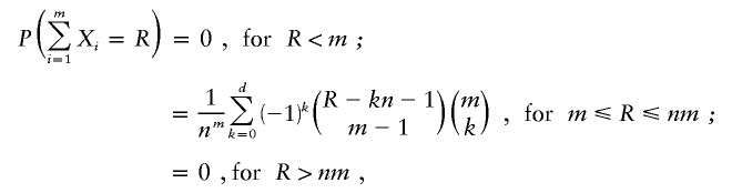where R is summed rank, X_i is the rank of study i, m is the number of studies, n is the number of bins (120), and d is the integer part of (R-m)/n. For unweighted analyses, pointwise P values for R can be determined directly from this distribution, although, for weighted analyses, a permutation procedure is required, as described above.

It is mathematically equivalent to rank bins in descending order and to average rather than sum the ranks across bins. For any R, the equivalent average ascending rank R_avg is: (n+1)-(R/m). Results have been expressed this way in the current article to provide a more intuitive terminology.

Appendix C: Summary of Terminology

Bin:

One of 120 30-cM autosomal segments used as units of analysis in GSMA; bin 2.1 is the first 30 cM of chromosome 2.

R_study (within-study rank):

The rank of each bin within a single study, based on the maximum linkage score (or lowest P value) within it. The bin containing the best score has a rank of 1. All negative and 0 scores are considered to be tied. For weighted analyses, each raw rank is multiplied by the study’s weighting factor.

R_avg (average rank):

The average of a bin’s within-study ranks or weighted ranks across all studies.

P_AvgRnk (probability of R_avg):

The pointwise probability of observing a given R_avg for a bin in a GSMA of N studies, determined by theoretical distribution (unweighted analysis only) or by permutation test (fig. 2).

P_ord (probability of R_avg given the order):

The pointwise probability that, for example, a 1st-place, 2nd-place, 3rd-place, etc., bin would achieve R_avg at least this extreme in a GSMA of N studies.

Genomewide significance:

For α=0.05, correction for 120 bins yields a threshold for genome-wide significance of .000417 for P_AvgRnk or P_ord. For suggestive linkage (a result observed once per scan by chance), α=1/120=0.0083.

Appendix D: Criteria for Genomewide Significance

For individual bins, the criterion for genomewide significance is P_AvgRnk<.000417. When linkage is likely to be present in one or more bins, the aggregate criteria are as follows: ⩾11 bins with P_AvgRnk<.000417, ⩾4 bins with P_ord<.05 among the 10 best values of R_avg, or ⩾5 bins with P_AvgRnk<.05 and P_ord<.05. Bins with P_AvgRnk<.05 and P_ord<.05 are most likely to contain linked loci. No valid combined significance criterion was identified.

References

- ——— (2002a) Meta-analysis of whole-genome linkage scans of bipolar disorder and schizophrenia. Mol Psychiatry 7:405–411 [DOI] [PubMed] [Google Scholar]
- Badner JA, Gershon ES (2002b) Regional meta-analysis of published data supports linkage of autism with markers on chromosome 7. Mol Psychiatry 7:56–66 [DOI] [PubMed] [Google Scholar]
- Berrettini WH (2000) Are schizophrenic and bipolar disorders related? A review of family and molecular studies. Biol Psychiatry 48:531–538 [DOI] [PubMed] [Google Scholar]
- Dorr D, Rice J, Armstrong C, Reich T, Blehar M (1997) A meta-analysis of chromosome 18 linkage data for bipolar illness. Genet Epidemiol 14:617–622 [DOI] [PubMed] [Google Scholar]
- Gill M, Vallada H, Collier D, Sham P, Holmans P, Murray R, McGuffin P, et al (1996) A combined analysis of D22S278 marker alleles in affected sib-pairs: support for a susceptibility locus for schizophrenia at chromosome 22q12. Schizophrenia Collaborative Linkage Group (Chromosome 22). Am J Med Genet 67:40–45 [DOI] [PubMed] [Google Scholar]
- Göring HHH, Terwilliger JD, Blangero J (2001) Large upward bias in estimation of locus-specific effects from genome-wide scans. Am J Hum Genet 69:1357–1369 [DOI] [PMC free article] [PubMed] [Google Scholar]
- Hauser ER, Boehnke M, Guo SW, Risch N (1996) Affected sib-pair interval mapping and exclusion for complex genetic traits: sampling considerations. Genet Epidemiol 13:117–138 [DOI] [PubMed] [Google Scholar]
- James JW (1971) Frequency in relatives for an all-or-none trait. Ann Hum Genet 35:47–49 [DOI] [PubMed] [Google Scholar]
- Kong A, Gudbjartsson DF, Sainz J, Jonsdottir GM, Gudjonsson SA, Richardsson B, Sigurdardottir S, Barnard J, Hallbeck B, Masson G, Shlien A, Palsson ST, Frigge ML, Thorgeirsson TE, Gulcher JR, Stefansson K (2002) A high-resolution recombination map of the human genome. Nat Genet 31:241–247 [DOI] [PubMed] [Google Scholar]
- Kruglyak L, Daly M (1998) Linkage thresholds for two-stage genome scans. Am J Hum Genet 62:994–996 [DOI] [PMC free article] [PubMed] [Google Scholar]
- Kruglyak L, Daly MJ, Reeve-Daly MP, Lander ES (1996) Parametric and nonparametric linkage analysis: a unified multipoint approach. Am J Hum Genet 58:1347–1363 [PMC free article] [PubMed] [Google Scholar]
- Lander E, Kruglyak L (1995) Genetic dissection of complex traits: guidelines for interpreting and reporting linkage results. Nat Genet 11:241–247 [DOI] [PubMed] [Google Scholar]
- Levinson DF, Holmans P, Straub RE, Owen MJ, Wildenauer DB, Gejman PV, Pulver AE, Laurent C, Kendler KS, Walsh D, Norton N, Williams NM, Schwab SG, Lerer B, Mowry BJ, Sanders AR, Antonarakis SE, Blouin JL, DeLeuze JF, Mallet J (2000) Multicenter linkage study of schizophrenia candidate regions on chromosomes 5q, 6q, 10p, and 13q: schizophrenia linkage collaborative group III. Am J Hum Genet 67:652–663 [DOI] [PMC free article] [PubMed] [Google Scholar]
- Levinson DF, Mowry BJ (2000) Genetics of schizophrenia. In: Pfaff DW, Berrettini WH, Maxson SC, Joh TH (eds) Genetic influences on neural and behavioral functions. CRC Press, New York, pp 47–82 [Google Scholar]
- Lewis CM, Levinson DF, Wise LH, DeLisi LE, Straub RE, Hovatta I, Williams NM, et al (2003) Genome scan meta-analysis of schizophrenia and bipolor disorder, part II: schizophrenia. Am J Hum Genet 73:34–48 (in this issue) [DOI] [PMC free article] [PubMed] [Google Scholar]
- North BV, Curtis D, Sham PC (2002) A note on the calculation of empirical P values from Monte Carlo procedures. Am J Hum Genet 71:439–441 [DOI] [PMC free article] [PubMed] [Google Scholar]
- Risch N (1987) Assessing the role of HLA-linked and unlinked determinants of disease. Am J Hum Genet 40:1–14 [PMC free article] [PubMed] [Google Scholar]
- ——— (1990) Linkage strategies for genetically complex traits. I. Multilocus models. Am J Hum Genet 46:222–228 [PMC free article] [PubMed] [Google Scholar]
- Schizophrenia Linkage Collaborative Group for Chromosomes 3, 6 and 8 (1996) Additional support for schizophrenia linkage on chromosomes 6 and 8: a multicenter study. Am J Med Genet 67:580–594 [DOI] [PubMed] [Google Scholar]
- Segurado R, Detera-Wadleigh SD, Levinson DF, Lewis CM, Gill M, Nurnberger JI Jr, Craddock N (2003) Genome scan meta-analysis of schizophrenia and bipolar disorder, part III: bipolar disorder. Am J Hum Genet 73:49–62 (in this issue) [DOI] [PMC free article] [PubMed] [Google Scholar]
- Wise LH, Lanchbury JS, Lewis CM (1999) Meta-analysis of genome searches. Ann Hum Genet 63:263–272 [DOI] [PubMed] [Google Scholar]