Recurrent Fourier-Kolmogorov Arnold Networks for photovoltaic power forecasting

Abstract

Accurate day-ahead forecasting of photovoltaic (PV) power generation is crucial for power system scheduling. To overcome the inaccuracies and inefficiencies of current PV power generation forecasting models, this paper introduces the Recurrent Fourier-Kolmogorov Arnold Network (RFKAN). Initially, recurrent kernel nodes are employed to investigate the interdependencies within sequences. Subsequently, Fourier series are applied to extract periodic features, enhancing forecasting accuracy and training speed. Ablation studies conducted using data from a PV power plant in Tieling City, Liaoning Province, validate the effectiveness of these two structural enhancements. Comparative experiments with baseline and state-of-the-art models further underscore the efficiency of RFKAN. The results indicate that RFKAN achieves the best forecasting performance with a grid depth of 100 and an input sequence length of 2, reducing RMSE and MAE by at least 5%, increasing CORR by 2%, and decreasing training time by 24% compared to advanced models.

Introduction

As the exploitation of fossil fuels intensifies and global environmental issues worsen, many countries are adopting strategies to harness solar energy^1–3. Photovoltaic (PV) power generation stands out as a clean, low-carbon, and sustainable form of renewable energy^4–6. As a decentralized energy source, solar power contributes to meeting local electricity demands, especially during grid operations. Unlike other renewable sources, PV generation typically coincides with daylight hours, matching peak electricity usage⁷. With careful power dispatching, the distribution network can effectively utilize solar energy resources to meet daytime load demands. In this context, obtaining accurate PV generation forecasts in advance is crucial^8–10, as the precision of these forecasts significantly impacts power dispatching strategies¹¹.

The output of PV generation is heavily influenced by variables such as light intensity, temperature, humidity, and weather patterns, leading to considerable volatility and unpredictability^12–15. As a result, precise forecasting of PV power for the following day is imperative^16,17. The importance of day-ahead PV forecasting in power dispatch cannot be overstated, as its benefits significantly surpass those of ultra-short-term forecasting. Day-ahead forecasts provide a longer preparation window, which is essential for ensuring the stable functioning of the power grid¹⁸. Consequently, there is an urgent requirement for the development of a novel model that offers both high prediction accuracy and computational efficiency.

Related works and contributions

Related works

PV forecasting is crucial for effective power dispatch, yet the volatility and non-stationarity of PV power series present significant forecasting challenges. In response to these challenges, numerous scholars have conducted extensive research and proposed a variety of time series forecasting models. The primary forecasting models proposed thus far include (1) physical models¹⁹, (2) statistical models²⁰, and (3) artificial intelligence models²¹. Physical models are estimated with parameters such as wind speed, pressure, topography, and temperature²². However, their heavy dependence on weather and the need for numerous costly parameters limit their universal applicability²³. Advancements in science and technology have led to the widespread exploration of statistical methods like linear regression²⁴, ARIMA²⁵, and probabilistic statistics²⁶, but they can be less robust with missing data and nonlinearities²⁷.

Artificial intelligence has emerged as the cornerstone of PV forecasting, with deep learning outpacing traditional neural networks and machine learning models in the age of big data. This shift is particularly pronounced in the domain of ultra-short-term PV forecasting, where recent academic research has propelled significant advancements²⁸. At the forefront of these developments, the introduction of an Adaptive Masked Network has elevated the precision of PV forecasts to new heights, achieving cutting-edge performance on three renowned public PV power datasets²⁹. In parallel, the synergy of deep learning with cloud computing technologies has been harnessed to not only enhance the accuracy but also to improve the computational efficiency of existing PV forecasting methodologies³⁰. Furthermore, a self-coupled transformer model, which incorporates quadratic decomposition, Bayesian optimization, and error correction, has been validated using four months of data from a solar plant in Hangzhou, China, showcasing its predictive capabilities³¹. The PLSTNet model, grounded in deep learning, has also emerged as a high-accuracy forecaster for ultra-short-term PV power across diverse scenarios³². Transformer model has been adapted for PV power prediction, underscoring its versatility³³. In a novel approach, the QK-CNN leverages a CNN architecture with four distinct kernel sizes to extract local cross-features within sequences, which are then refined by a single-kernel CNN to effectively capture temporal dynamics and achieve remarkable forecasting results³⁴. The DS-CNN has demonstrated exceptional performance in predicting PV power across various time scales and seasonal conditions³⁵. Transfer learning and the K-nearest neighbor algorithm have been integrated into the C-LSTM model to forecast PV power for newly installed plants, while the GRU neural network has also been applied to PV power prediction with high accuracy^36,37. Finally, a modified Transformer architecture has been proposed to simultaneously forecast PV and wind power generation, with a comparative analysis underscoring the model’s superiority against the latest technologies³⁸.

These models are surpassing benchmarks in complex forecasting, driving the need for more advanced network architectures. However, inspired by Multilayer Perceptron (MLP), they often face scalability issues since the number of parameters does not increase linearly with additional layers. To address these challenges, Reference³⁹ introduces Kolmogorov-Arnold Networks (KAN), a neural architecture based on the Kolmogorov-Arnold theorem. KAN’s key innovation is the use of spline-based univariate functions as learnable activation functions at the network edges, replacing the traditional linear weights. While KAN successfully reduces the parameter count, it encounters difficulties in effectively extracting sequence interdependencies and struggles with fitting periodic sequences, leading to suboptimal forecasting performance. This study builds upon the KAN framework to develop the Recurrent Fourier-Kolmogorov Arnold Network (RFKAN), inspired by Recurrent Neural Network (RNN). RFKAN replaces the challenging-to-train splines with manageable Fourier series, adeptly identifying and extracting time series dependencies to enhance prediction accuracy while maintaining computational efficiency.

Contributions

In order to improve accuracy and efficiency of PV forecasting, RFKAN is proposed in this study and the main contributions and novelties are summarized as follows.

1. RFKAN is ingeniously crafted to correlate input nodes with the output from the preceding time step, effectively harnessing the short-term dependencies within the time series.

2. To accelerate the training of PV sequences, Fourier series are used instead of Spline sample while keeping the grid features unchanged.

3. The validity of the model is verified by ablation experiments and comparison tests of multiple models under different seasons.

Model principles and architecture

Overall architecture of RFKAN

This paper introduces RFKAN, designed to enhance the precision of PV forecasting and guarantee efficient model training. Drawing on KAN, the research substitutes spline function with Fourier series to better fit the highly periodic nature of PV data and incorporates RNN architecture to encapsulate short-term dependencies in time-series information. PV dataset x has structure , where represents the length of time series and represents the number of feature at each temporal node. Thus the number of input normal nodes n is . In this study, two layer RFKAN is used and its structure is shown in Fig. 1.

Fig. 1.

Structure of RFKAN.

As shown in Fig. 1, parameter of recurrent kernel nodes are first obtained through RNN architecture. In this step, input sequence dimension n is equal to the number of normal and recurrent nodes. Two types of nodes are fed in parallel to Layer 1. Second, in Layer 1, a Fourier sequence of crude grid is used for learning by the network to generate 2n + 1 normal nodes. Then, RNN architecture is again utilized to obtain recurrent kernel nodes with same number of nodes as normal nodes and feed these nodes into Layer 2 having same grid size as Layer 1. Finally, prediction results for crude grid are given. Further, after crude grid training is completed, RFKAN inherits its learnable activation function curve. Subsequently, RFKAN is trained more precisely through a finely grained grid to improve the accuracy of the forecasting results.

KAN

KAN is based on Kolmogorov-Arnold representation theorem, which shows that any multivariate continuous function can be represented as a composite form of univariate functions with additive operations. The structure of KAN is shown in Fig. 2.

Fig. 2.

Structures of KAN.

According to Fig. 2, KAN can be expressed as:

1

where is a function that maps each input univariate , such as and .

The function of KAN layer is shown in Eq. (2):

2

where is a learnable parametric function.

In Kolmogov-Arnold theorem, internal functions form a KAN layer with and and external functions form a KAN layer with and . In Eq. (1) is expressed a simple combination of two KAN layers. The extension of KAN and the implementation of spline function can be found in reference³⁹

Design of RNN structure

RNN is adept at processing time-series data and capturing long-range dependencies. Drawing inspiration from RNN architecture, KAN incorporates a recurrent kernel structure that endows the network with dynamic temporal processing capabilities. This is achieved by integrating past hidden states into the current state, thereby preserving a memory of historical input information. RNN structure is shown in Fig. 1. and proof of the role of this node is given in section "Impact of model architecture". In KAN, each transform function is modified to be related to time. Define as historical memory function that captures the moment of node in layer , which is given in Eq. (3)

3

Output of layer is shown in Eq. (4):

4

In matrix, this can be expressed as:

5

6

The final output of KAN is shown in Eq. (7):

7

Design of Fourier series

The core principle of KAN is the superposition of multiple nonlinear functions to construct an arbitrary function. However, training a KAN is more challenging than training a MLP because the number of parameters needed for spline functions depends on the number of data points and the spline’s degree of freedom, which complicates the training process. Nonetheless, the objective can be attained by decomposing a complex function into several simpler nonlinear functions. Fourier series, with their capacity to encapsulate the data’s characteristics across the entire period using a limited number of parameters, offer a global representation of the periodic data once the parameters are established. The structure of Fourier series is shown in Fig. 1. and proof of the role of this node is given in "Impact of model architecture" section. Fourier series offer a significant computational efficiency advantage, which helps to overcome the training difficulties presented by spline functions. Equation (8) is an alternative to spline function:

8

where is feature dimension. and are trainable parameters. is grid size.

Results and discussion

Data description and evaluation metrics

Data description

In this study, the dataset from Tieling City, Liaoning Province, was selected and analyzed using actual PV power generation and weather data for the entire year of 2023 (365 days). The weather data primarily included temperature, relative humidity, cloud cover, solar irradiance, wind speed, and wind direction, with a data sampling interval of 5 min. This resulted in a total of 105,120 sample points. The maximum capacity of the power plant in this area is 45 kW. Table 1 provides sample data on environmental factors and PV power.

Table 1.

Partial sample of data obtained on environmental factors.

Environmental factors	2023/1/3/ 12:00	2023/1/3/ 12:05	2023/1/3/ 12:10	2023/1/3/ 12:15	… …
Temperature	− 8.5632°	− 8.5535°	− 8.4629°	− 8.4396°	… …
Humidity	54.2365%	54.2562%	54.2598%	54.2613%
Cloud cover	13.5%	13.5%	13.5%	13.5%
Solar irradiance	364.31W/m2	365.65W/m2	368.93W/m2	369.67W/m2
Wind speed	3.3m/s	3.3m/s	3.3m/s	3.3m/s
Wind direction	North	North	North	North
PV power	36.8008	36.6141	36.5602	36.5685

Before PV data is input to RFKAN, it needs to be preprocessed to eliminate the effect of defects in the data itself on prediction results. For categorical variables, binary coding preprocessing method is used and the coding is shown in Table 2. For continuous variables, the processing steps are as follows:

1. Default value filling: Utilizing linear interpolation to fill in missing values of PV data based on data from adjacent time points to ensure data continuity.

2. Outlier detection: Irradiation 0–1000 W/m², power generation greater than 0, maximum power less than installed capacity. The outlier data is judged abnormal and processed by linear interpolation.

3. Data normalization: in order to reduce negative effects on network training due to differences in data sizes, the data are uniformly mapped to the [0,1] range.

Table 2.

Binary coding of wind direction.

Wind direction	Binary code
North	000
North-East	001
East	010
South-East	011
South	100
South-West	101
West	110
North-West	111

To prevent data leakage, the training and test datasets are split in chronological order, ensuring that the training set comprises only data points that precede those in the test set. In ablation studies, data from May 10th is randomly designated as the test sample, with the remainder used for training. To evaluate the model’s predictive performance across various seasonal conditions more precisely, the data is segmented by season. Test samples are randomly selected for spring (March 10th), summer (June 11th), autumn (September 2nd), and winter (December 20th). This approach accounts for the potential influence of seasonal changes on PV power generation, thereby enhancing the accuracy of the model’s evaluation.

Evaluation metrics

To objectively assess RFKAN, this paper employs three widely recognized metrics: Mean Absolute Error (MAE)⁴⁰, Root Mean Square Error (RMSE)⁴¹, and R Squared index (CORR)⁴². While the overnight PV power is not the focus of detailed analysis, it is still included in the plots to ensure data continuity. The formulas for these metrics are presented in Eq. (9).

9

where: is the length of forecast sequence, is the actual value of PV power at points, is forecast value of PV power at n points, and is the average power of PV power.

In evaluating model performance, smaller values of MAE and RMSE indicate higher forecasting accuracy. As CORR value nears 1, model fit improves, indicating better performance.

Ablation experiments

Impact of model architecture

This section conducts ablation studies to quantitatively evaluate the unique influence of each enhancement component on the efficacy of RFKAN. A sequence of four experiments is designed to examine the individual contributions of different architectural changes to RFKAN.

1. First, KAN baseline model experiments are conducted, and this step provides an important reference benchmark for subsequent comparative analysis of other models.

2. FKAN model is constructed, which is based on RFKAN by removing the RNN structure at the nodes.

3. RKAN model is constructed, which is based on RFKAN by removing the Fourier series part but retaining RNN architecture.

4. RFKAN model integrates RNN architecture with the Fourier series to validate the effectiveness of this innovative combination.

The forecasting results of KAN, FKAN, RKAN, and RFKAN are depicted in Fig. 3. A notable discrepancy in predictive performance among the models is observed around noon. KAN is inadequate in fitting periodic time series data, particularly at noon, where the prediction accuracy significantly decreases. Concurrently, KAN fails to effectively harness the influence of historical data on current data, leading to substantial prediction errors at points of volatility. In contrast to KAN, RKAN excels in capturing sequence dependencies due to the incorporation of RNN architecture, yet it struggles to capture the periodic relationships within the sequences. Conversely, FKAN effectively captures the periodic dependencies of the sequences but lacks the ability to extract inter-sequence dependencies, resulting in insufficient accuracy when forecasting fluctuation points. RFKAN is achieved by combining the Fourier series with RNN architecture in KAN. It effectively captures the dependencies between sequences. It also identifies the periodic features of the sequences. This combination results in the most accurate predictive outcomes.

Fig. 3.

Ablation experiment forecasting results.

To evaluate model performance more comprehensively, Table 3 demonstrates the evaluation metrics of each model in ablation experiments.

Table 3.

Forecasting indicators for each model.

Model	RMSE	MAE	CORR	Running time/s
KAN	5.4265	3.0141	0.8679	4125.84
RKAN	4.3688	2.6427	0.9246	4793.62
FKAN	4.1829	2.7677	0.9192	3125.84
RFKAN	3.4168	1.6146	0.9461	3519.38

According to Table 3, KAN exhibits the least favorable forecasting performance. The integration of RNN architecture into KAN results in a noticeable improvement in forecasting indices, highlighting the RNN’s effectiveness in capturing temporal dependencies and thereby enhancing the precision of PV power forecasts. It is important to acknowledge, however, that the inclusion of RNN adds to the model’s computational complexity. Furthermore, the incorporation of Fourier series into KAN not only boosts forecasting performance but also reduces training time by 24.24%, demonstrating the Fourier series’ rapid adaptability to periodic data. Nonetheless, the forecasting metrics for this enhanced model still fall slightly short of those achieved by RKAN. The simultaneous application of both RNN architecture and Fourier series to KAN results in a comprehensive enhancement of its forecasting indices. The RMSE and MAE are reduced by 37.03% and 46.43%, respectively, and CORR increases by 8.27%. Additionally, the training time is decreased by 14.69%.

Effect of RFKAN grid parameters

In RFKAN, grid size significantly impacts performance. Smaller grids enhance detail capture and accuracy but boost computational complexity. Larger grids speed up processing but may sacrifice detail and accuracy. Striking a balance between precision and efficiency is crucial. RFKAN starts with a larger grid, then refines it every 50 steps. Figure 4 shows RFKAN’s performance and runtime across different grid sizes.

Fig. 4.

RFKAN model index (left) and model runtime (right) for different grid depths.

The left side of Fig. 4 clearly indicates that after every 50 steps, RMSE loss value drops significantly with each grid refinement, highlighting the close relationship between RFKAN accuracy and grid refinement level. However, the right side of Fig. 4 reveals a sharp increase in runtime when the grid depth surpasses 100 levels. Moreover, analyzing the data on the left side, we observe that over-refinement of the grid can actually degrade RFKAN forecasting performance. Consequently, this study opts to cap the grid depth at 100 levels to achieve a balance between forecasting performance and computational efficiency.

Effect of number of input nodes

A fundamental principle of RFKAN is to approximate complex relationships with a learnable activation function. Consequently, varying the number of input nodes, which corresponds to different lengths of temporal feature sequences, necessitates different learnable activation functions. With a grid cutoff depth set at 100 and an output sequence length of 288 (spanning two days of PV data), the influence of varying input sequence lengths (from 1 to 288) on RFKAN forecasting efficacy was investigated. Figure 5 shows that the training time for models other than RFKAN escalates exponentially with the length of the input sequence, without a proportional enhancement in forecasting accuracy. The study’s findings suggest that when the input data length is 2, RFKAN introduced in this research demonstrates superior performance across all forecasting metrics and training duration, surpassing the capabilities of other models.

Fig. 5.

Evaluation metrics change for four models with different input sequence lengths.

The three sets of ablation experiments conducted above have yielded the optimal parameters for RFKAN, as detailed in Table 4. Subsequent experiments were carried out using these established parameters.

Table 4.

RFKAN model parameters.

Parameter	Value	Parameter	Value
Step	50	Grid	[3,5,10,20,50,100]
K	3	Input nodes	12
Input seq_len	12	Recurrent kernel nodes	12

Evaluation of predictive models

Comparison with base model

To evaluate the effectiveness of RFKAN, five baseline models have been chosen for comparative analysis within this study. These baseline models cover different technical areas, including traditional regression models (ARIMA), machine learning models (SVM and ELM), and deep learning models (LSTM and TCN). The parameters of each comparison model are shown in Table 5. As Table 4 shows, RFKAN performs 50 iterations on each grid and is carried out 6 times, so the number of iterations for each comparison model is 300.

Table 5.

Comparison model parameters.

Model	Parameter	Value
ARIMA	AR order	2
	Differencing order	1
	MA order	1
SVM	Kernel	RBF
	C	0.0043
ELM	Number of hidden layer	3
	Activation function	ReLU
	Regularization coefficient	0.001,
LSTM	Number of hidden layer	3
	Learning rate	0.001
	Batch size	32
	Activation function	ReLU
	Optimizer	Adam
TCN	Number of convolutional layers	3
	Stride	2
	Padding	Same
	Activation function	ReLU

To comprehensively evaluate the forecasting capabilities of these models across various seasonal patterns, separate experiments were conducted for each season. Figure 6 illustrates the forecasting performance of each model throughout different seasons, and overall performance metrics are consolidated in Table 6.

Fig. 6.

Forecasting performance of each base model in different seasons.

Table 6.

Overall performance metrics of different seasonal base models.

Season	Model	RMSE	MAE	CORR	Running time/s
Spring	ARIMA	10.3218	8.2115	0.5626	302.53
	ELM	8.2618	6.7361	0.7048	352.19
	SVM	8.4750	6.6850	0.7343	364.27
	GRU	7.4038	6.0887	0.7740	946.71
	TCN	7.4442	6.1409	0.7807	1041.38
	RFKAN	3.0740	1.8341	0.9534	1145.52
Summer	ARIMA	8.3971	6.3171	0.7388	298.62
	ELM	7.4807	6.0629	0.7891	348.91
	SVM	7.4476	6.0240	0.7931	360.68
	GRU	6.9229	5.6609	0.8148	937.61
	TCN	6.2250	5.1759	0.8609	1031.37
	RFKAN	2.5744	1.5144	0.9655	1134.51
Autumn	ARIMA	8.3530	6.2945	0.7414	296.08
	ELM	7.4523	6.0292	0.7926	346.08
	SVM	7.4673	6.0443	0.7912	358.08
	GRU	6.7236	5.5552	0.8239	931.08
	TCN	6.2246	5.1747	0.8610	1024.19
	RFKAN	2.6706	1.5782	0.9620	1126.52
Winter	ARIMA	8.8900	7.0724	0.6563	301.46
	ELM	8.3943	6.4075	0.7329	351.53
	SVM	8.4250	6.4658	0.7259	363.61
	GRU	7.3176	6.0329	0.7934	945.36
	TCN	7.4209	6.1075	0.7842	1039.89
	RFKAN	3.4168	1.6146	0.9511	1143.88

Figure 6 analysis reveals that forecasting metrics for models (excluding RFKAN) worsen in spring and winter versus summer and autumn, likely due to regional weather variability. Table 6 indicates that statistical and machine learning models underperform in forecasting, exposing their limitations in handling irregular data. While GRU and TCN excelled in feature extraction and demonstrated high forecasting accuracy, RFKAN outperformed all models with the best predictive results. Compared to the other five base models, RFKAN reduced RMSE by at least 58.64%, MSE by at least 70.74%, and improved CORR by at least 10.31%. Training duration across models remained largely consistent seasonally. Despite the model proposed here requiring the most training time, its superior predictive capabilities confirm it as the optimal selection.

Comparison with advanced models

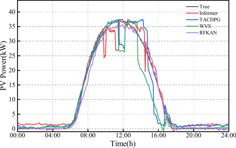
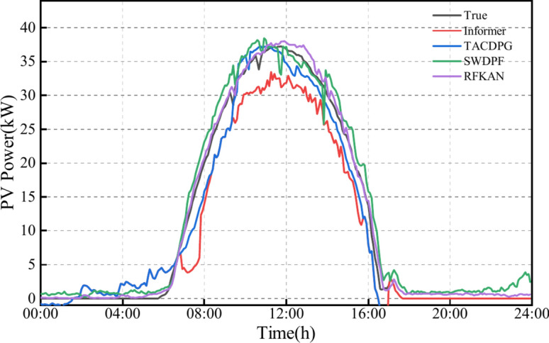
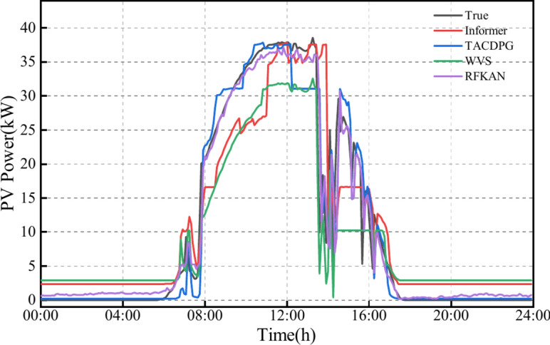
This study further benchmarks the proposed RFKAN against three sophisticated models: Informer⁴³, WVS⁴⁴, and TACDPG⁴⁵. The parameters for each model are consistent with those reported in the respective literature. This approach facilitates a precise evaluation of RFKAN relative forecasting capabilities. To guarantee a thorough and equitable comparison, all models are tested and assessed using the same dataset and experimental conditions. The detailed outcomes of the forecasting performance comparison are presented in Fig. 7, with the specific forecasting metrics detailed in Table 7.

Fig. 7.

Forecasting performance of advanced models in different seasons.

Table 7.

Overall performance indicators of advanced models in different seasons.

Season	Model	RMSE	MAE	CORR	Running time/s
Spring	Informer	4.02853	2.2023	0.9058	1653.62
	WVS	4.1661	2.3039	0.904	1719.19
	TACDPG	4.1971	2.3053	0.9039	1496.32
	RFKAN	3.074	1.8341	0.9534	1145.52
Summer	Informer	3.8513	2.0935	0.9166	1633.76
	WVS	3.3525	1.9018	0.9401	1732.69
	TACDPG	3.6419	2.0186	0.9279	1600.49
	RFKAN	2.5744	1.5144	0.9655	1134.51
Autumn	Informer	3.8244	2.0533	0.9182	1700.45
	WVS	3.4317	2.0084	0.9371	1856.32
	TACDPG	3.5897	2.0363	0.9341	1532.61
	RFKAN	2.6706	1.5782	0.9621	1126.52
Winter	Informer	3.8471	2.1042	0.91567	1698.66
	WVS	3.6205	2.1308	0.9312	1811.11
	TACDPG	3.7323	2.0977	0.9237	1512.65
	RFKAN	3.4168	1.6146	0.9511	1143.88

Figure 7 and Table 7 reveal that RFKAN outperforms other models in PV forecasting. It maintains stable forecasting indicators with minimal fluctuations, cutting RMSE by at least 5.57% and MSE by 24.22% compared to advanced models, while enhancing CORR by at least 2.09%. RFKAN also demonstrates the highest training efficiency, with a training time that is 24.37% shorter than its counterparts. These results underscore the significant advantages and efficiency of RFKAN in PV forecasting. For a more direct comparison of the forecasting performance of the different models, Figs. 8, 9, 10, 11 visually present the forecasting outcomes for each model.

Fig. 8.

Spring forecast results.

Fig. 9.

Results of the summer forecast.

Fig. 10.

Autumn forecast results.

Fig. 11.

Winter forecast results.

PV power trend is generally stable during summer and autumn, with the models’ predicted curves closely aligning with actual power generation. However, springtime peak hours see significant fluctuations in PV power generation, and winter afternoons also exhibit greater volatility. All comparative models show some prediction bias due to unpredictable changes in external environmental factors. Informer selectively ignores certain elements in sequences, assuming intrinsic sparsity, but this can lead to an inability to fully account for highly correlated characteristics between sequence elements, negatively impacting its performance during PV data fluctuations.

TACDPG employs a decay function to optimize the reward function, but later training stages may prioritize short-term gains over long-term patterns, resulting in poor predictions during significant PV power fluctuations. When WVS uses VMD smoothing for data decomposition, it can remove noise but may also discard crucial time-series features, particularly during abrupt weather changes. This filtering can lead to a marked decrease in the model’s predictive effectiveness during periods of fluctuation.

Additionally, RFKAN, represented by the purple line, closely matches the actual data’s black line. This is largely due to its RNN architecture, which effectively captures both long-term and short-term dependencies. By incorporating the Fourier series technique, the model further extracts the periodicity of the PV sequences. RFKAN proposed in this study demonstrates exceptional stability and accuracy in PV power prediction tasks.

Conclusion and future work

Accurate forecasting of PV power is crucial for power system operations. This paper introduces RFKAN, a day-ahead PV forecasting framework that leverages RNN architecture and incorporates Fourier series. RFKAN comprises: (1) recurrent kernel nodes for sequence interdependency, boosting accuracy, and (2) Fourier series for rapid extraction of periodic features, reducing training time. The forecasting capabilities of RFKAN are assessed using data from the Tieling PV power plant located in Liaoning Province.

1. Ablation studies affirm the critical role of RNN structure in bolstering sequence dependency extraction, as well as the efficiency of Fourier series in quickly identifying cyclical features and its robust fitting capacity.

2. Ablation studies have investigated the effects of different grid depths on RFKAN forecasting capabilities, as well as the influence of input sequence length on forecast accuracy. The results show that RFKAN achieves optimal forecasting at a grid depth of 100. Similarly, RFKAN best performance is observed with an input sequence length of 2.

3. RFKAN introduced in this paper outperforms both the base and advanced models across all seasons, achieving at least a 5% decrease in RMSE and MAE, and a 2% increase in CORR. Furthermore, RFKAN training time is 24% shorter than advanced model.

In essence, RFKAN demonstrates consistent performance, offering valuable insights for power system planning. Future studies will focus on the influence of data precision on model efficacy and the consequences of data drift on its predictive powers.

Author contributions

Z.L. wrote the body of the manuscript and D.R. and G.X. checked the paper. All authors reviewed the manuscript.

Funding

Funding was provided by National Natural Science Foundation of China (Grant no: 62373260), Shenzhen Science and Technology Program (Grant no: 20231127173014002).

Data availability

The data that support the findings of this study are available from Liaoning Tieling Power Supply Company but restrictions apply to the availability of these data, which were used under license for the current study, and so are not publicly available. Data are however available from the corresponding authors upon reasonable request and with permission of Liaoning Tieling Power Supply Company.

Declarations

Competing interests

The authors declare no competing interests.

References

- 1.Engineering - Industrial Engineering. Study data from north China electric power university provide new insights into industrial engineering (weather-classification-mars-based photovoltaic power forecasting for energy imbalance market). J. Eng. (2019).
- 2.Abdel-Nasser, M. & Mahmoud, K. Accurate photovoltaic power forecasting models using deep LSTM-RNN. Neural Comput. Appl.31(7), 2727–2740 (2019). [Google Scholar]
- 3.Douiri, R. M. Particle swarm optimized neuro-fuzzy system for photovoltaic power forecasting model. Solar Energy184, 91–104 (2019). [Google Scholar]
- 4.Donghun, L. & Kwanho, K. PV power prediction in a peak zone using recurrent neural networks in the absence of future meteorological information. Renew. Energy. (2020) (prepublish).
- 5.Xifeng, G. et al. Study on short-term photovoltaic power prediction model based on the stacking ensemble learning. Energy Rep.6(S9), 1424–1431 (2020). [Google Scholar]
- 6.Ying, Z. & Laiqiang, K. Photovoltaic power prediction based on hybrid modeling of neural network and stochastic differential equation. ISA Trans.128(Pt B), 181–206 (2022). [DOI] [PubMed] [Google Scholar]
- 7.Bo, G. et al. Forecasting and uncertainty analysis of day-ahead photovoltaic power using a novel forecasting method. Appl. Energy299, 117291 (2021). [Google Scholar]
- 8.Zhiying, L. et al. A method of ground-based cloud motion predict: CCLSTM + SR-Net. Remote Sens.13(19), 3876–3876 (2021). [Google Scholar]
- 9.Koster, D. et al. Short-term and regionalized photovoltaic power forecasting, enhanced by reference systems, on the example of Luxembourg. Renew. Energy132, 455–470 (2019). [Google Scholar]
- 10.Pan, M. et al. Photovoltaic power forecasting based on a support vector machine with improved ant colony optimization. J. Clean. Prod.277, 123948 (2020). [Google Scholar]
- 11.Huixin, M. et al. An integrated framework of gated recurrent unit based on improved sine cosine algorithm for photovoltaic power forecasting. Energy256, 124650 (2022). [Google Scholar]
- 12.Syed, M. I. & Raahemifar, K. Energy advancement integrated predictive optimization of photovoltaic assisted battery energy storage system for cost optimization. Electr. Power Syst. Res.140, 917–924 (2016). [Google Scholar]
- 13.Barbieri, F., Rajakaruna, S. & Ghosh, A. Very short-term photovoltaic power forecasting with cloud modeling: a review. Renew. Sustain. Energy Rev.75, 242–263 (2016). [Google Scholar]
- 14.Nonita, S. et al. A sequential ensemble model for photovoltaic power forecasting. Comput. Electr. Eng.96(PA), 107484 (2021). [Google Scholar]
- 15.Zhou, Y. et al. Prediction of photovoltaic power output based on similar day analysis, genetic algorithm and extreme learning machine. Energy.204, 117894 (2020). [Google Scholar]
- 16.Hao, Z. et al. Photovoltaic power forecasting based on GA improved Bi-LSTM in microgrid without meteorological information. Energy231, 120908 (2021). [Google Scholar]
- 17.Zheng, L. et al. Short-term photovoltaic power prediction based on modal reconstruction and hybrid deep learning model. Energy Rep.8, 9919–9932 (2022). [Google Scholar]
- 18.Yongju, S. et al. LSTM–GAN based cloud movement prediction in satellite images for PV forecast. J. Ambient Intell. Human. Comput.14(9), 12373–12386 (2022). [Google Scholar]
- 19.Yuan, Z., Tao, S. & Xudong, Y. A physical model with meteorological forecasting for hourly rooftop photovoltaic power prediction. J. Build. Eng.75, 106997 (2023). [Google Scholar]
- 20.Wang, J. et al. A short-term photovoltaic power prediction model based on the gradient boost decision tree. Appl. Sci.8(5), 689 (2018). [Google Scholar]
- 21.Xie, G. & Lin, Z. RSMD-RF-BGSkip based PV generation prediction method. IEEE Access12, 65799–65809. 10.1109/ACCESS.2024.3398033 (2024). [Google Scholar]
- 22.Wang, H. et al. Short-term photovoltaic power forecasting based on a feature rise-dimensional two-layer ensemble learning model. Sustainability15(21), 15594 (2023). [Google Scholar]
- 23.Sonja, K. & Monica, S. Photovoltaic power prediction for solar micro-grid optimal control. Energy Rep.9(S1), 594–601 (2023). [Google Scholar]
- 24.Wengen, G. & Qigong, C. An Bayesian learning and nonlinear regression model for photovoltaic power output forecasting. Appl. Math. Nonlinear Sci.5(2), 531–542 (2020). [Google Scholar]
- 25.Song, D., Ruojin, L. & Zui, T. A novel adaptive discrete grey model with time-varying parameters for long-term photovoltaic power generation forecasting. Energy Convers. Manag.227, 113644 (2021). [Google Scholar]
- 26.Ahmad, T. et al. Enhancing probabilistic solar PV forecasting: integrating the NB-DST method with deterministic models. Energies17(10), 2392 (2024). [Google Scholar]
- 27.Xiyun, Y. et al. Short-term photovoltaic power prediction with similar-day integrated by BP-AdaBoost based on the Grey-Markov model. Electr. Power Syst. Res.215(PA), 108966 (2023). [Google Scholar]
- 28.Li, R. et al. Short-term photovoltaic prediction based on CNN-GRU optimized by improved similar day extraction, decomposition noise reduction and SSA optimization. IET Renew. Power Gener.18(6), 908–928 (2024). [Google Scholar]
- 29.Ma, Q. et al. Adaptive masked network for ultra-short-term photovoltaic forecast. Eng. Appl. Artif. Intell.139(PB), 109555–109555 (2025). [Google Scholar]
- 30.Zhaolong, Z. Intelligent prediction method for power generation based on deep learning and cloud computing in big data networks. Int. J. Intell. Netw.4, 224–230 (2023). [Google Scholar]
- 31.Chen, J. et al. An error-corrected deep Autoformer model via Bayesian optimization algorithm and secondary decomposition for photovoltaic power prediction. Appl. Energy377(PD), 124738–124738 (2025). [Google Scholar]
- 32.Li, G. et al. Research on a novel photovoltaic power forecasting model based on parallel long and short-term time series network. Energy293, 130621 (2024). [Google Scholar]
- 33.Zhao, X. A novel digital-twin approach based on transformer for photovoltaic power prediction. Sci. Rep.14(1), 26661–26661 (2024). [DOI] [PMC free article] [PubMed] [Google Scholar]
- 34.Xiaoying, R. et al. Quad-kernel deep convolutional neural network for intra-hour photovoltaic power forecasting. Appl. Energy323, 119682 (2022). [Google Scholar]
- 35.Chen, R. Z., Bai, L. Y. & Hong, T. J. Constructing two-stream input matrices in a convolutional neural network for photovoltaic power prediction. Eng. Appl. Artif. Intell.135, 108814 (2024). [Google Scholar]
- 36.Xing, L., Dongxiao, Z. & Xu, Z. Combining transfer learning and constrained long short-term memory for power generation forecasting of newly-constructed photovoltaic plants. Renew. Energy185, 1062–1077 (2022). [Google Scholar]
- 37.Su, Z. et al. Improving ultra-short-term photovoltaic power forecasting using advanced deep-learning approach. Measurement239, 115405–115405 (2025). [Google Scholar]
- 38.Feroz, A. M. et al. Quantile-transformed multi-attention residual framework (QT-MARF) for medium-term PV and wind power prediction. Renew. Energy220, 119604 (2024). [Google Scholar]
- 39.Liu, Z. et al. Kan: Kolmogorov-Arnold networks arXiv preprint arXiv:2404.19756 (2024).
- 40.Zhao, X. et al. A new short-term wind power prediction methodology based on linear and nonlinear hybrid models. Comput. Ind. Eng.196, 110477–110477 (2024). [Google Scholar]
- 41.Sun, B., Su, M. & He, J. Wind power prediction through acoustic data-driven online modeling and active wake control. Energy Convers. Manag.319, 118920–118920 (2024). [Google Scholar]
- 42.Hu, M. et al. Short-term wind power prediction based on improved variational modal decomposition, least absolute shrinkage and selection operator, and BiGRU networks. Energy303, 131951 (2024). [Google Scholar]
- 43.Ma, S. et al. Forecasting air quality Index in Yan’an using temporal encoded informer. Expert Syst. Appl.255(PD), 124868–124868 (2024). [Google Scholar]
- 44.Zhao, Y. et al. WOA-VMD-SCINet: Hybrid model for accurate prediction of ultra-short-term photovoltaic generation power considering seasonal variations. Energy Rep.12, 3470–3487 (2024). [Google Scholar]
- 45.Zhang, R. et al. Deep reinforcement learning based interpretable photovoltaic power prediction framework. Sustain. Energy Technol. Assess.67, 103830 (2024). [Google Scholar]
Associated Data
This section collects any data citations, data availability statements, or supplementary materials included in this article.
Data Availability Statement