

Abstract
Extreme discordant sibling pairs (EDSPs) are theoretically powerful for the mapping of quantitative-trait loci (QTLs) in humans. EDSPs have not been used much in practice, however, because of the need to screen very large populations to find enough pairs that are extreme and discordant. Given appropriate statistical methods, another alternative is to use moderately discordant sibling pairs (MDSPs)—pairs that are discordant but not at the far extremes of the distribution. Such pairs can be powerful yet far easier to collect than extreme discordant pairs. Recent work on statistical methods for QTL mapping in humans has included a number of methods that, though not developed specifically for discordant pairs, may well be powerful for MDSPs and possibly even EDSPs. In the present article, we survey the new statistics and discuss their applicability to discordant pairs. We then use simulation to study the type I error and the power of various statistics for EDSPs and for MDSPs. We conclude that the best statistic(s) for discordant pairs (moderate or extreme) is (are) to be found among the new statistics. We suggest that the new statistics are appropriate for many other designs as well—and that, in fact, they open the way for the exploration of entirely novel designs.
Introduction
The extreme discordant sibling pair (EDSP) design is generally attributed to Risch and Zhang (1995). The basic idea of the EDSP design is that, if phenotyping is relatively easy, then one can screen a large population of sibling pairs and genotype only those pairs that are most powerful for the detection of linkage. The simplest version of the design uses only those pairs in which one sibling has a trait value in the top 10% of the trait distribution and the other sibling has a trait value in the bottom 10% of the trait distribution. The EDSP idea was further developed in articles such as those by Risch and Zhang (1996), Gu et al. (1996), Kruse et al. (1997), Rogus et al. (1997), and Knapp (1998). These authors studied the power of several variations on EDSP sampling, including the extreme discordant and concordant (EDAC) design, which includes pairs in which both siblings are in the top 10% or both siblings are in the bottom 10%. Despite theoretical development, the EDSP and EDAC designs have only occasionally been used in practice. Only those investigators who have very large populations to work with and relatively low phenotyping costs have found such studies to be practical. For example, Xu et al. (1999) screened >200,000 people in Anqing, China, to ascertain 207 extreme discordant and 357 extreme concordant pairs for blood pressure, and Fullerton et al. (2003) screened 20,427 independent sibships to get a final data set of 182 discordant and 379 concordant pairs for neuroticism.
The reason for the historical emphasis on extreme discordant pairs has to do with the statistical test that is used to detect linkage. In a standard EDSP study, one tests for linkage by estimating the average number of alleles shared identical by descent (IBD) between the pairs at a marker. If the marker locus is linked to the trait, then the mean IBD-sharing score should be less than the null-hypothesis expectation. This is the same test statistic (tested in the opposite direction) as is used for affected-sibling-pair mapping of binary disease traits (e.g., see Blackwelder and Elston 1985). However, the IBD-sharing statistic is not very powerful unless the pairs are drawn from the extremes of the distribution. This is because the power of the statistic comes purely from the fact that the trait values are extreme; it does not use the actual trait values in any way.
More recently, the suggestion has been made that one can use different statistics for discordant pairs—statistics that not only use information about the IBD sharing but also incorporate information about the trait values. Such statistics can make it possible to use less extreme samples and might make discordant-pair studies more practical. Forrest and Feingold (2000) suggested using a composite statistic that is a weighted sum of the IBD-sharing statistic and the Haseman and Elston (1972) statistic. The composite statistic is only slightly more powerful than the IBD-sharing statistic for EDSP samples, but the advantage is greater for moderately discordant sibling pairs (MDSPs), defined arbitrarily by Forrest and Feingold (2000) as pairs with one sibling in the top 35% of the distribution and one sibling in the bottom 35% of the distribution. The existence of a powerful statistic for MDSPs makes it possible to consider that design as a compromise between EDSPs and population sampling. For example, under one trait model that Forrest and Feingold (2000) studied, one could achieve 80% power by screening 8,700 pairs to ascertain 55 EDSPs, or by screening 1,850 pairs to ascertain 300 MDSPs, or by using a population sample of 950 pairs.
In addition to the Forrest and Feingold (2000) composite statistic, there are several other recent methods that may also be applicable to discordant pairs. In the present article, we survey those statistics and then use simulation to compare their type I error and power with those of the IBD-sharing statistic. In the “Methods” section, we discuss statistics for discordant pairs in more detail and define the statistics that we consider in the present article. We then describe our simulation methods and present our results. We conclude with a discussion of the implication of our results for other study designs.
Methods
Statistics Considered
Discordant and concordant pairs have a property that makes them critically different from more typical samples—they have a distorted IBD-sharing distribution at markers that are linked to the trait. Sibling pairs from a population sample are expected to share half of their alleles IBD at any locus, regardless of whether that locus is linked to the trait being studied. The same is true if the pairs are sampled on the basis of a single individual with an extreme trait value. However, if families are sampled on the basis of a criterion that looks at two or more members (which we refer to as “multiple-proband ascertainment”), then the IBD-sharing distribution changes at a marker linked to the trait. In the companion article (T.Cuenco et al. 2003 [in this issue]), we sampled pairs in which at least one sibling exceeds a threshold; this actually qualifies as multiple-proband ascertainment (because both phenotypes must be seen in order to decide whether to ascertain the pair) but changes the IBD-sharing distribution only very slightly. In the case of discordant and concordant pairs, the change in the IBD-sharing distribution is quite substantial, and this is exactly what Risch and Zhang’s (1995) original EDSP method sought to detect. Nonetheless, the IBD-sharing statistic for EDSP pairs is limited in that it looks only at the IBD sharing, ignoring the actual trait values.
Conversely, most standard human QTL-mapping methods, which were developed with population samples in mind, do not look at the marginal distribution of IBD sharing at all; rather, they base their power on the detection of correlation between the IBD sharing of each pair and the similarity of the pair's trait values. Hereafter, we refer to such statistics as “correlation-based statistics.” Haseman-Elston regression (Haseman and Elston 1972) and maximum-likelihood variance components (e.g., see Amos 1994) are the most commonly used examples of correlation-based methods.
The set of correlation-based statistics has recently been expanded quite a bit, with attempts to update the Haseman-Elston method (Drigalenko 1998; Elston et al. 2000; Xu et al. 2000; Forrest 2001; Sham and Purcell 2001; Visscher and Hopper 2001). There are also several new statistics in the literature that combine information from both the marginal IBD-sharing distribution and the correlation (Sham et al. 2000, 2002; Sham and Purcell 2001; Tang and Siegmund 2001; Putter and Sandkuijl 2002; Wang and Huang 2002). These statistics should be appropriate for discordant pairs, and they should be more powerful than statistics that rely only on IBD or only on correlation.
All of the new statistics are described in brief below and are reviewed in more detail by Feingold (2001, 2002).
Risch and Zhang's IBD-sharing statistic (IBD1).—Let πi be the estimated mean IBD sharing for sibling pair i; πi takes the value 0, 1/2, or 1 for a fully informative pair but can take intermediate values if multipoint estimates are used. Let  be the average estimated IBD sharing over all pairs in the sample. The classical linkage test based on EDSPs (Risch and Zhang 1995) uses the statistic
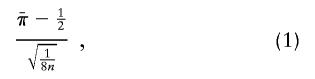 |
which is  standardized to have mean 0 and variance 1. A one-sided Z test is used to detect significantly negative values. The SD in the denominator is a theoretical value that assumes that IBD information for each pair is observed perfectly (i.e., that the marker is infinitely polymorphic). This results in a conservative test when this statistic is applied to real data in which IBD sharing is estimated from marker data (for discussion of this issue in the context of affected sibling pairs, see Davis and Weeks 1997).
Robust IBD-sharing statistic (IBD2)
Instead of the denominator used above, in equation (1), the IBD-sharing statistic can also be standardized using an empirical SD, which yields the statistic
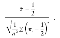 |
The test based on this statistic should have correct type I error even if the IBD information is not perfectly observed. One could also consider replacing the factor of 1/2 in the denominator with  , which should result in a very slightly elevated type I error and power.
Original Haseman-Elston (ORIGINAL.HE)
Let YiD=(xi1-xi2)2 be the squared trait difference for sibling pair i. The method of Haseman and Elston (1972) simply regresses YiD on πi and estimates the slope, −βD. A positive estimate for βD (a negative estimate for the slope) suggests that the trait is linked to the locus marker. A one-sided t test is used to test for any significant departure from 0.
Trait-sum regression (TRAIT.SUM)
Let YiS=[(xi1-μ)+(xi2-μ)]2 be the mean-corrected squared trait sum. We include the one-sided t test of the slope  from the regression of YiS on πi.
Trait-product regression (TRAIT.PRODUCT)
Under population sampling,  and
and  are estimates of the same parameter (Drigalenko 1998). This slope parameter should be 0 under the null hypothesis of no linkage and should be positive (as we have defined the sign) under the alternative hypothesis. Drigalenko (1998) suggested averaging the two slope estimates—or, equivalently, doing a single regression with the mean-corrected trait product, (Xi1-μ)(Xi2-μ), as the dependent variable. We consider the one-sided t test based on the trait-product regression.
Forrest‘s method (FORREST)
Forrest (2001) suggested a test based on the weighted average
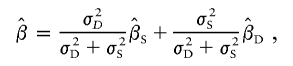 |
where σ2D and σ2S are the variances of  and
and  . These weights are optimal under the assumption that the covariance, σ2DS, of
  is 0, which is true for a population sample from a normal distribution but which is not necessarily true otherwise (Feingold 2002). FORREST estimates all the parameters simultaneously, using iterative least squares.
Visscher and Hopper’s method (V&H)
Visscher and Hopper (2001) proposed a test based on the same weighted slope estimate as Forrest (2001) but with the two variances estimated separately, by performing the two regressions separately.
Xu et al.’s method (XU)
Xu et al. (2000) proposed a method very similar to that of Forrest (2001) and Visscher and Hopper (2001), but their weighted average slope allows for a nonzero covariance between  and
and  , using the formula
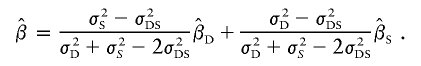 |
Xu et al. estimate the parameters by performing the two regressions separately, similar to V&H. The covariance can be estimated by combining the residuals of the two regressions.
Sham and Purcell’s method (S&P1)
The variances σ2D and σ2S can actually be calculated analytically as functions of the sibling trait correlation, r, under traditional QTL models. Sham and Purcell (2001) proposed taking advantage of this, rather than estimating the variances from data as in FORREST, V&H, and XU. The primary method outlined by Sham and Purcell (2001) regresses the dependent variable
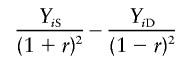 |
on πi, where the trait values xi1 and xi2 are standardized to mean 0 and variance 1 before calculation of YiS and YiD.
Sham and Purcell’s robust method (S&P2)
Sham and Purcell (2001) also suggested a variant of their method, regressing
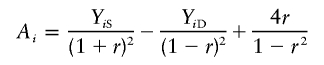 |
on πi- 1/2, with the intercept fixed at 0. This variant should be more robust to selected sampling. Even more important, it implicitly incorporates information on any distortion in the IBD sharing. This is because the fixed intercept implies a null-hypothesis IBD-sharing proportion of 1/2, so the regression t test draws power from any deviation from that proportion. The t statistic for the test of the regression slope is
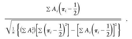 |
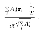
Asymptotic score statistic (SCORE1)
Score statistics based on the usual variance-components likelihood were proposed by Tang and Siegmund (2001), Wang and Huang (2002), and Putter et al. (2002). The score statistics proposed in their articles are very similar to each other but have minor differences in how they parameterize the likelihood and how they “robustify” the statistic. Instead of considering precisely the statistics in the aforementioned articles, we take the Tang and Siegmund (2001) statistic as our starting point and consider four variations on possible ways to make it robust (or not). Tang and Siegmund (2001) derived a score statistic of the form
 |
where Ai is the same function as defined above for S&P2. The denominator of this statistic is based on asymptotic likelihood theory, so this version of the score statistic is not expected to be appropriate for discordant sibling pairs.
Score statistic with partially empirical variance (SCORE2)
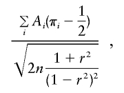
Tang and Siegmund (2001) proposed making their statistic robust by using the empirical SD of Ai in the denominator—that is,
 |
The factor of  is the SD of π when a perfectly informative marker is assumed. Thus, this version of the statistic should be appropriate for discordant pairs but should yield a conservative test when there is imperfect IBD information.
Score statistic with fully empirical variance (SCORE3)
We propose that the best version of the score statistic should have the same form as SCORE2 but with the empirical SD of π in place of the factor of  :
:
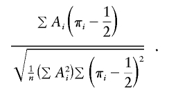 |
This version should have correct type I error even with imperfect IBD information. As with IBD2, it is also possible here to replace the factor of 1/2 in the denominator with  , which would give slightly higher type I error and power.
Score statistic with empirical mean and variance (SCORE4)
Both Wang and Huang (2002a) and Putter et al. (2002) proposed using  in place of 1/2 in both the numerator and denominator of the score statistic. When applied to our parameterization of the score statistic, that yields the expression
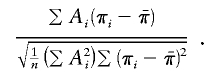 |
The use of the empirical mean IBD sharing in the numerator means that this version of the score statistic does not draw any power from the distortion in IBD sharing in discordant pairs, similar to S&P1 (whereas SCORE3 is similar to S&P2).
Composite statistic (COMPOSITE1)
Forrest and Feingold (2000) proposed testing for linkage by using a weighted average of ORIGINAL.HE and IBD1:
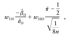 |
where wHE and wIBD are arbitrarily chosen weights. On the basis of limited calculations, they recommended that MDSPs be analyzed using equal weights and that EDSPs be analyzed using a higher weight on the IBD-sharing statistic. We use equal weights in the present article. Any of the correlation-based statistics can be used in place of ORIGINAL.HE in the composite. Forrest and Feingold (2000) found that, for discordant pairs, ORIGINAL.HE was the most powerful choice in the literature at that time. In updating that investigation with all of the correlation-based statistics, we found that ORIGINAL.HE was still the most powerful, so we implemented COMPOSITE1 as above. Note that the IBD-sharing component of COMPOSITE1 is standardized using the theoretical variance, so it is expected to be conservative when there is imperfect IBD-sharing information.
Empirical composite statistic (COMPOSITE2)
The composite can also be formed as the average of ORIGINAL.HE and IBD2 (instead of IBD1). This version should have correct type I error even when there is not perfect IBD information.
* * *
In our presentation of the results, the statistics we call “group A” (IBD1 and IBD2) are versions of the traditional IBD-sharing statistic. The group B statistics (ORIGINAL.HE, TRAIT.SUM, TRAIT.PRODUCT, XU, V&H, FORREST, S&P1, and SCORE4) are the correlation-based statistics; they do not consider the marginal IBD-sharing distribution. The group C statistics (S&P2, SCORE1, SCORE2, SCORE3, COMPOSITE1, and COMPOSITE2) are the statistics that consider both IBD sharing and correlation.
We are aware of two other statistics that fall into group C but that we did not include in our study because of computational limitations. One is the ascertainment-corrected variance-components statistic proposed by Sham et al. (2000), which conditions on trait values; this statistic should perform very similarly to SCORE3 and S&P2. The other statistic that we did not include is the regression-based statistic proposed by Sham et al. (2002); this statistic was developed for extended pedigrees, but, for sibling pairs, it takes the same form as SCORE2 and SCORE3, except that the variance of π is estimated differently.
Many of the statistics that we evaluated depend on estimates of trait parameters. TRAIT.SUM, TRAIT.PRODUCT, XU, V&H, FORREST, S&P1, S&P2, SCORE1, SCORE2, SCORE3, and SCORE4 all use an estimate of the trait mean, μ. The S&P statistics and the SCORE statistics additionally use estimates of the trait variance, σ2, and the sibling correlation, r. Sensitivity to these estimates may have an important effect on power.
Simulations
We studied the type I error and the power of each statistic under seven trait models, which are described in table 1. All of the models are diallelic. Models 1–5 are simple mixture-of-normals models; the trait value is equal to the genotype mean plus a normally distributed “environmental” variance. There is an additional sibling correlation of 0.25 in each model, to account for environmental and polygenic components. The means and the variances were chosen to give each model a locus heritability of 0.2. Models 1′ and 2′ were generated by simulating data under models 1 and 2, respectively, and then taking the signed square,  , of each trait value. This yields overall trait distributions that are somewhat skewed and have high kurtosis. Model 3 also has skewness and kurtosis in the same ranges as models 1′ and 2′. Note that models 6–9 from the companion article (T.Cuenco et al. 2003 [in this issue]) were not used here, because, for discordant pair sampling, they are symmetric with other models.
Table 1.
Genetic Models[Note]
|
Value for Model |
|||||||
| Parameter | 1 | 2 | 3 | 4 | 5 | 1′ | 2′ |
| Model-defining: | |||||||
| Type of inheritancea | Add | Dom | Rec | Add | Dom | Add | Dom |
| Locus heritability | .2 | .2 | .2 | .2 | .2 | NA | NA |
| Allele frequency | .1 | .1 | .1 | .5 | .5 | .1 | .1 |
| Trait means | −1, 0, 1 | 0, 1, 1 | 0, 0, 1 | −1, 0, 1 | 0, 1, 1 | −1.6, 0, 1.6 | 0, 1.6, 1.6 |
| Environmental SD | .849 | .785 | .199 | 1.414 | .866 | NA | NA |
| Environmental correlation | .25 | .25 | .25 | .25 | .25 | NA | NA |
| Calculated: | |||||||
| Overall mean | −.8 | .19 | .01 | .0 | .75 | −1.32 | .295 |
| Overall SD | .949 | .877 | .222 | 1.581 | .968 | 2.047 | 1.393 |
| Skewness | .166 | .141 | .885 | .0971 | −.0991 | −1.587 | 1.504 |
| Kurtosis | .0989 | .0235 | 3.814 | .0556 | −.0714 | 5.268 | 9.406 |
| Overall correlation | .3 | .3 | .3 | .3 | .3 | .25 | .26 |
Note.— NA = not applicable.
Add = additive; Dom = dominant; Rec = recessive.
Under each of the models, we simulated data for nuclear families with two children, and we ascertained families by two different methods. The first ascertainment scheme was based on EDSPs—any pair in which one sibling was in the top 10% of the trait distribution and the other sibling was in the bottom 10%. The second scheme was based on MDSPs—any pair in which one sibling was in the top 35% and the other sibling was in the bottom 35%. We simulated data sets of 100 families for the EDSP samples and 500 families for the MDSP samples. Figure 1 shows examples of simulated bivariate trait distributions for both sampling schemes under several of the models. To study type I error, we used 10,000 data sets, and, to study power, we used 1,000 data sets. The nominal type I error rate was set at 0.01. Marker data was simulated using eight equifrequent alleles, with the marker at recombination fraction (θ) 0 for the power study and at θ=0.5 for the type I error study. We also did power simulations at θ=0.05 for models 1 and 2 only.
Figure 1.

Scatterplots of population, MDSP, and EDSP samples from models 1, 2, and 1′
As discussed above (see the “Statistics Considered” subsection), most of the statistics require that some trait parameters (mean μ, variance σ2, and sibling correlation r) be specified. In general, theory suggests that these should be population parameter values, even for selected samples. However, if one is using a selected sample, population parameter estimates may not be available. In that situation, parameter values must be guessed or adopted from previous studies in other populations. Using models 1 and 1′ only, we examined the robustness of the statistics to misspecification of parameters. We varied one parameter at a time while holding the other two parameters at the correct population values. Sibling correlation was set at 0.1 and 0.5, trait variance was set at values ranging from half the true value to twice the true value, and trait mean was set at the true mean ± 1 SD. We also did a limited number of studies in which two parameters at a time were misspecified. Finally, we checked the performance of the statistics by using sample estimates of the parameters.
Results
Type I Error
Table 2 shows the SD and type I error of each statistic, based on the 10,000 simulated data sets with EDSP samples. All statistics had mean 0 for all models. All of the statistics in this table were computed with the known population values of the parameters (trait mean μ, variance σ2, and sibling correlation r). The 95% CI for an estimated error rate of 1.00% is ∼0.80%–1.20%. As expected, the statistics that assume perfect IBD information (IBD1, SCORE2, and COMPOSITE 1) have conservative type I error. V&H and FORREST also have incorrect type I error, presumably because of the omission of the covariance term in the weighting. Finally, SCORE1 and SCORE4 have incorrect type I error. These results are qualitatively consistent across all models and are also true for the MDSP samples (results not shown). The incorrect type I error for SCORE4 is due to covariance terms that are omitted from the denominator of that statistic (for discussion, see T.Cuenco et al. 2003 [in this issue]). S&P2 and SCORE3 are very similar, with S&P2 having a slightly higher type I error rate for most models. We did limited experiments (results not shown) with versions of SCORE3, IBD2, and COMPOSITE2 that replaced 1/2 in the denominator with  (see the “Methods” section). This increases the type I error of those methods by 0.1–0.2 percentage points for the models that we studied.
Table 2.
SD and Type I Error for EDSP Samples
|
SD and Type I Error under Model |
||||||||||||||
| 1 |
2 |
3 |
4 |
5 |
1′ |
2′ |
||||||||
| Statistic | SD | Error(%) | SD | Error(%) | SD | Error(%) | SD | Error(%) | SD | Error(%) | SD | Error(%) | SD | Error(%) |
| Group A: | ||||||||||||||
| IBD1 | .93 | .60 | .93 | .69 | .93 | .76 | .93 | .77 | .94 | .71 | .93 | .73 | .93 | .76 |
| IBD2 | 1.00 | .98 | 1.00 | .95 | 1.00 | 1.06 | 1.00 | 1.14 | 1.01 | .99 | 1.00 | .97 | 1.01 | 1.05 |
| Group B: | ||||||||||||||
| ORIGINAL.HE | 1.00 | .96 | 1.01 | 1.13 | 1.02 | 1.22 | 1.00 | 1.03 | 1.02 | 1.05 | 1.01 | 1.06 | 1.01 | .82 |
| TRAIT.SUM | 1.00 | .95 | 1.01 | .99 | 1.02 | 1.06 | 1.01 | .91 | 1.00 | .97 | 1.02 | 1.13 | 1.01 | .84 |
| TRAIT.PRODUCT | 1.00 | 1.00 | 1.01 | 1.10 | 1.02 | 1.12 | 1.00 | 1.12 | 1.02 | 1.04 | 1.01 | 1.18 | 1.00 | .98 |
| XU | 1.00 | 1.10 | 1.00 | .98 | .95 | .80 | 1.01 | 1.09 | 1.01 | 1.10 | .98 | .89 | .98 | .88 |
| V&H | .75 | .15 | .75 | .17 | .39 | .00 | .76 | .15 | .78 | .13 | .49 | .01 | .54 | .02 |
| FORREST | .93 | .62 | .94 | .66 | .74 | .07 | .94 | .63 | .94 | .66 | .66 | .10 | .74 | .10 |
| S&P1 | 1.00 | .98 | 1.01 | 1.15 | 1.02 | 1.22 | 1.00 | 1.05 | 1.02 | 1.07 | 1.01 | 1.08 | 1.01 | .87 |
| SCORE4 | .31 | .00 | .31 | .00 | .62 | .00 | .30 | .00 | .30 | .00 | .54 | .00 | .62 | .00 |
| Group C: | ||||||||||||||
| S&P2 | 1.02 | 1.05 | 1.02 | 1.19 | 1.02 | 1.17 | 1.01 | 1.25 | 1.03 | 1.23 | 1.02 | 1.16 | 1.02 | 1.21 |
| SCORE1 | 4.61 | 30.34 | 4.56 | 30.34 | 6.10 | 34.96 | 4.36 | 30.37 | 4.65 | 30.69 | 3.99 | 28.56 | 4.80 | 31.75 |
| SCORE2 | .93 | .60 | .93 | .67 | .93 | .61 | .93 | .70 | .94 | .70 | .93 | .60 | .93 | .56 |
| SCORE3 | 1.00 | .92 | 1.00 | 1.02 | 1.00 | 1.05 | 1.00 | 1.10 | 1.01 | 1.03 | 1.00 | .92 | 1.01 | .99 |
| COMPOSITE1 | .96 | .76 | .97 | .90 | .97 | .83 | .96 | .91 | .98 | .96 | .97 | .75 | .97 | .73 |
| COMPOSITE2 | 1.00 | .92 | 1.00 | 1.10 | 1.01 | 1.05 | 1.00 | 1.10 | 1.01 | 1.19 | 1.01 | .97 | 1.01 | .98 |
Power
Table 3 gives the power for all models for the EDSP samples, and table 4 gives the power for the MDSP samples. Again, all of the statistics in these tables were computed with the known population values of the parameters. To make comparisons simpler, we omitted from the power tables the statistics that did not have correct type I error. The 95% CI for a power estimate of 50% is ∼47%–53%.
Table 3.
Power for EDSP Samples
|
Power under Model |
|||||||
| Statistic | 1 | 2 | 3 | 4 | 5 | 1′ | 2′ |
| Group A: | |||||||
| IBD2 | .82 | .91 | .05 | .92 | .78 | .81 | .84 |
| Group B: | |||||||
| ORIGINAL.HE | .11 | .05 | .18 | .08 | .04 | .05 | .04 |
| TRAIT.SUM | .00 | .00 | .00 | .00 | .01 | .01 | .00 |
| TRAIT.PRODUCT | .11 | .05 | .17 | .08 | .05 | .07 | .04 |
| XU | .01 | .01 | .00 | .02 | .01 | .06 | .01 |
| S&P1 | .12 | .05 | .18 | .08 | .05 | .06 | .04 |
| Group C: | |||||||
| S&P2 | .88 | .94 | .21 | .94 | .83 | .81 | .80 |
| SCORE3 | .87 | .93 | .18 | .94 | .81 | .78 | .79 |
| COMPOSITE2 | .79 | .78 | .22 | .81 | .62 | .66 | .71 |
Table 4.
Power for MDSP Samples
|
Power under Model |
|||||||
| Statistic | 1 | 2 | 3 | 4 | 5 | 1′ | 2′ |
| Group A: | |||||||
| IBD2 | .41 | .50 | .02 | .63 | .58 | .45 | .52 |
| Group B: | |||||||
| ORIGINAL.HE | .38 | .32 | .15 | .33 | .30 | .10 | .28 |
| TRAIT.SUM | .00 | .00 | .00 | .00 | .00 | .00 | .00 |
| TRAIT.PRODUCT | .34 | .31 | .10 | .34 | .28 | .14 | .27 |
| XU | .03 | .03 | .00 | .04 | .02 | .10 | .06 |
| S&P1 | .37 | .32 | .15 | .34 | .29 | .11 | .30 |
| Group C: | |||||||
| S&P2 | .73 | .77 | .13 | .84 | .79 | .43 | .64 |
| SCORE3 | .72 | .77 | .12 | .84 | .79 | .42 | .64 |
| COMPOSITE2 | .73 | .77 | .11 | .83 | .78 | .49 | .74 |
For the EDSP samples, it is clear that most of the linkage information is in the marginal IBD-sharing distribution, with only a small amount in the correlation between IBD and trait differences. The group B statistics, which rely only on correlation, have very little power. IBD2 and the group C statistics all have very similar power. COMPOSITE2 has somewhat lower power than the other group C statistics, because we computed it with equal weights on the IBD statistic and the Haseman-Elston statistic. If COMPOSITE2 were computed with the weights suggested by Forrest and Feingold (2000) for EDSPs, it would probably have similar power to S&P2 and SCORE3. Interestingly, S&P2 and SCORE3 do have slightly higher power than IBD2, except against models 1′ and 2′, for which they have slightly lower power. This suggests that the most nonparametric statistic may do better against nonnormal trait models.
For the MDSP samples, the group C statistics are again the most powerful. In this case, COMPOSITE2 performs very similarly to S&P2 and SCORE3, presumably because the weighting that we used to form the composite is, in fact, the weighting that Forrest and Feingold (2000) recommended for MDSPs. IBD2 has somewhat lower power, reflecting that the group C statistics are drawing power from both the marginal IBD-sharing distribution and the IBD/trait-difference correlation. COMPOSITE2 outperforms S&P2 and SCORE3 precisely on the nonnormal models.
We did limited experiments (results not shown) with versions of SCORE3, IBD2, and COMPOSITE2 that replaced 1/2 in the denominator with  (see the “Methods” section). The altered SCORE3 has power very similar to that of S&P2. The altered IBD2 and COMPOSITE2 statistics also gain 1–2 percentage points in power. We also did power simulations at θ=0.05 for models 1 and 2 only (results not shown); although the overall power is lower than at θ=0, the relative power of the different statistics is unchanged.
Sensitivity
To assess the robustness of the statistics to misspecification of the trait parameters, we first tried using the sample parameter values for each data set, rather than the known correct values. The basic effect for both EDSP and MDSP samples is to cut the power of the S&P1, S&P2, and SCORE3 statistics to 0 (results not shown). IBD2, ORIGINAL.HE, and COMPOSITE2 do not use the parameter values at all, so they are unaffected.
A more realistic sensitivity analysis is to use parameter values that are guessed with error. We investigated the effect of misspecifying one parameter at a time. For each run, we set two of the parameters to the population values and set the third to an arbitrary “wrong guess” (see the “Methods” section). We performed these simulations on the same two data sets, one from model 1 and one from model 1′. Tables 5–8 present these results. For each table, we generated a single set of 1,000 data sets and analyzed them under different assumed parameter values. Table 5 shows power results for model 1 under EDSP sampling, table 6 shows the results for model 1′ under EDSP sampling, and tables 7 and 8 give the corresponding results for MDSP sampling. The type I error was correct for all of these sensitivity studies (results not shown).
Table 5.
Power for EDSP Samples—Sensitivity Analyses under Model 1
|
Power, Assuming |
|||||||
| Statistic | r=.1 | r=.5 | μ=-1.75 | μ=.15 | σ2=.45 | σ2=1.8 | Correct PopulationParameter Values |
| Group A: | |||||||
| IBD2 | .82 | .82 | .82 | .82 | .82 | .82 | .82 |
| Group B: | |||||||
| ORIGINAL.HE | .11 | .11 | .11 | .11 | .11 | .11 | .11 |
| TRAIT.SUM | .00 | .00 | .00 | .03 | .00 | .00 | .00 |
| TRAIT.PRODUCT | .11 | .11 | .04 | .13 | .11 | .11 | .11 |
| XU | .01 | .01 | .02 | .09 | .01 | .01 | .01 |
| S&P1 | .11 | .11 | .09 | .13 | .12 | .12 | .12 |
| Group C: | |||||||
| S&P2 | .88 | .88 | .88 | .89 | .88 | .88 | .88 |
| SCORE3 | .87 | .87 | .86 | .88 | .87 | .87 | .87 |
| COMPOSITE2 | .79 | .79 | .79 | .79 | .79 | .79 | .79 |
Table 6.
Power for EDSP Samples—Sensitivity Analyses under Model 1′
|
Power, Assuming |
|||||||
| Statistic | r=.1 | r=.5 | μ=-3.37 | μ=.73 | σ2=2.10 | σ2=8.38 | Correct PopulationParameter Values |
| Group A: | |||||||
| IBD2 | .81 | .81 | .81 | .81 | .81 | .81 | .81 |
| Group B: | |||||||
| ORIGINAL.HE | .05 | .05 | .05 | .05 | .05 | .05 | .05 |
| TRAIT.SUM | .01 | .01 | .00 | .02 | .01 | .01 | .01 |
| TRAIT.PRODUCT | .07 | .07 | .04 | .08 | .07 | .07 | .07 |
| XU | .06 | .06 | .00 | .08 | .06 | .06 | .06 |
| S&P1 | .07 | .06 | .05 | .06 | .06 | .06 | .06 |
| Group C: | |||||||
| S&P2 | .84 | .79 | .76 | .78 | .81 | .79 | .81 |
| SCORE3 | .82 | .77 | .75 | .76 | .79 | .77 | .78 |
| COMPOSITE2 | .66 | .66 | .66 | .66 | .66 | .66 | .66 |
Table 7.
Power for MDSP Samples—Sensitivity Analyses under Model 1
|
Power, Assuming |
|||||||
| Statistic | r=.1 | r=.5 | μ=-1.75 | μ=.15 | σ2=.45 | σ2=1.8 | Correct PopulationParameter Values |
| Group A: | |||||||
| IBD2 | .41 | .41 | .41 | .41 | .41 | .41 | .41 |
| Group B: | |||||||
| ORIGINAL.HE | .38 | .38 | .38 | .38 | .38 | .38 | .38 |
| TRAIT.SUM | .00 | .00 | .00 | .06 | .00 | .00 | .00 |
| TRAIT.PRODUCT | .34 | .34 | .03 | .39 | .34 | .34 | .34 |
| XU | .03 | .03 | .05 | .38 | .03 | .03 | .03 |
| S&P1 | .36 | .38 | .26 | .45 | .37 | .37 | .37 |
| Group C: | |||||||
| S&P2 | .71 | .73 | .60 | .75 | .72 | .73 | .73 |
| SCORE3 | .71 | .73 | .59 | .74 | .72 | .72 | .72 |
| COMPOSITE2 | .73 | .73 | .73 | .73 | .73 | .73 | .73 |
Table 8.
Power for MDSP Samples—Sensitivity Analyses under Model 1′
|
Power, Assuming |
|||||||
| Statistic | r=.1 | r=.5 | μ=-3.37 | μ=.73 | σ2=2.10 | σ2=8.38 | Correct PopulationParameter Values |
| Group A: | |||||||
| IBD2 | .45 | .45 | .45 | .45 | .45 | .45 | .45 |
| Group B: | |||||||
| ORIGINAL.HE | .10 | .10 | .10 | .10 | .10 | .10 | .10 |
| TRAIT.SUM | .00 | .00 | .00 | .00 | .00 | .00 | .00 |
| TRAIT.PRODUCT | .14 | .14 | .05 | .20 | .14 | .14 | .14 |
| XU | .10 | .10 | .01 | .34 | .10 | .10 | .10 |
| S&P1 | .12 | .10 | .07 | .21 | .11 | .11 | .11 |
| Group C: | |||||||
| S&P2 | .49 | .40 | .17 | .38 | .45 | .37 | .43 |
| SCORE3 | .48 | .40 | .17 | .37 | .44 | .36 | .42 |
| COMPOSITE2 | .49 | .49 | .49 | .49 | .49 | .49 | .49 |
For the EDSP samples from model 1 (table 5), misspecification of the trait parameters has no significant effect on the power of the group C statistics. This is because almost all of the power is coming from the IBD-sharing information, which does not depend on the parameters. Under model 1′ (table 6), the power is slightly more sensitive to parameter misspecification. This does not affect IBD2 and COMPOSITE2, because they do not use the parameter estimates. Note that misspecification actually increases power in some cases, presumably because the population trait value is the optimal choice only under normality assumptions.
Misspecification of the parameters has a larger effect for MDSP samples. Under model 1 (table 7), misspecification of the correlation or the variance does not have much effect, but misspecification of the mean can reduce the power of S&P2 and SCORE3, making COMPOSITE2 the most powerful statistic. Under model 1′ (table 8), misspecification of the variance or the correlation hurts the power of S&P2 and SCORE3 slightly, and misspecification of the mean cuts the power of those two statistics substantially. COMPOSITE2 is clearly the statistic with the most robust power for model 1′.
If one is adopting parameter estimates from a previous study, then it is likely that all three parameters will be incorrect by at least some margin. Since COMPOSITE2 and IBD2 do not use any parameter estimates, they should also be the most robust statistics for MDSPs and EDSPs, respectively, when there are errors in more than one parameter estimate. We did a limited study of the effects of misspecifying two parameters at a time. Detailed results are not shown, but the general qualitative result was that power was driven by how badly the mean was misspecified. This is consistent with the “one parameter wrong” runs described above, in which the mean had, by far, the greatest effect on power.
Discussion
We have reviewed a number of new sibling-pair QTL-mapping statistics and have investigated their appropriateness for discordant sibling pairs. For EDSPs, the best of the new statistics has only slightly higher power than the traditional IBD-sharing statistic, and the IBD-sharing statistic has the advantage of not depending on parameter estimates. For MDSPs, however, the statistics that combine IBD-sharing information and correlation information (i.e., the group C statistics) substantially outperform the IBD-sharing statistic. Of the group C statistics, COMPOSITE2 appears to be the most robust, having the highest power for nonnormal models and being independent of trait parameter estimates.
Our results for EDSPs and MDSPs are interesting, but they are only a small part of the story. The real importance of our results lies in two general conclusions that can be reached: the first is that any studies that use multiple-proband ascertainment would probably benefit from use of group C–type statistics; the second is that the existence of the group C statistics makes it possible to explore entirely new experimental designs. When the only statistic for discordant pairs was IBD sharing, the range of designs was limited essentially to different definitions of extreme discordance, but, with statistics that have robust ability to draw power from both the IBD sharing and the IBD/trait-value correlation, a much broader range of designs is possible. We have promoted the MDSP design as an option that might have the right balance of power and ease of ascertainment for some studies, but there are many other possibilities as well.
One way to think about new designs is to derive optimal designs for particular trait models. This approach was taken by Purcell et al. (2001), using the ascertainment-corrected variance-components statistic of Sham et al. (2000). Given a trait model, they identified the most informative 5% of pairs and showed that the power of that ascertainment scheme was far higher than that of other ways to choose 5% of pairs, even when the assumed trait model was wrong. Their method for identifying the most informative pairs could easily be applied to more moderate selection (e.g., 15% or 30%) as well. The approach could be carried even further by the assignment of ascertainment cost/difficulty numbers to different pairs and the selection of pairs to minimize total cost for a fixed amount of statistical power.
A very different way to think about new designs is to consider ascertainment schemes that are easy or convenient and study their power. For example, a low-effort way to recruit discordant pairs might be to select extreme probands that are already enrolled in a clinical study and then recruit any siblings that are in, say, the opposite half of the trait distribution. This could lead to discordant pairs defined as one sibling in the top 10% of the distribution and one sibling in the bottom 50% of the distribution. With flexible statistics, such ascertainment need not even be precise. For example, in the hypothetical design just described, it is unlikely that a clinically ascertained sample would actually be a random sample of the top 10% of the distribution; rather, it might be composed of any individuals whose trait values were relatively high (without a uniform cutoff) and whose physicians referred them. Using a statistic such as S&P2 or SCORE3 frees us to consider designs with such imprecise ascertainment without having to worry about the validity of the statistical analysis. COMPOSITE2 is probably not a good choice when ascertainment is imprecise, because it depends on arbitrary weights. The equal weights that we used performed very well for MDSPs as defined by Forrest and Feingold (2000), but the choice of good weights for any other particular design would require some art and advance planning.
One type of “convenience sample” that deserves further study includes affected sibling pairs already collected for linkage studies of binary traits. Affected sibling pairs can be considered concordant pairs for any quantitative traits associated with the disease that they were originally collected to study (e.g., glucose and insulin levels for diabetes). Sibling pairs collected for linkage have been used to map QTLs, but it has been done with correlation-based statistics (e.g., see Watanabe et al. 2000; Cai et al. 2001; Zhang et al. 2002). Such studies might, in theory, have much higher power with statistics, such as S&P2 and SCORE3, that can also get information from the marginal IBD-sharing distribution. Again, we do not recommend COMPOSITE2 for such nontraditional studies, because of the arbitrariness of the weights. It is also not clear whether the ORIGINAL.HE is the right correlation-based statistic to form the composite with for anything other than discordant pairs. Huang and Jiang (2003) recently proposed a likelihood-based statistic for the incorporation of quantitative-trait information into an affected-sibling-pair analysis, but it is not clear at this point how that method compares to the ones discussed here.
We did not explicitly study EDAC designs, but we believe that the same general results that we have shown for discordant pairs will hold. We expect that S&P2 and SCORE3 will have high and robust power. We suggest that variations on the EDAC design (e.g., choosing moderately discordant and concordant pairs) can be explored with those statistics.
We also recommend further study of designs that use larger sibships and even extended families that are selected on the basis of two or more members with extreme phenotypes. As long as the selection is based on two or more people, the alternative-hypothesis IBD sharing is affected, and it is almost certainly beneficial to use a statistic that can capture that information. There is plenty of evidence that larger sibships are more powerful than sibling pairs, even in the context of discordant designs. Alcais and Abel (2000) and Tang and Siegmund (2001) both showed that, if one has ascertained a discordant sibling pair, then it is most efficient to also use any other siblings in the sibship—more efficient than recruiting another independent discordant pair. The score statistics extend in a natural way to larger sibships and extended pedigrees and are probably the logical choice for studying and analyzing such designs. One problem that arises when a combination of pedigree types is used is that there may no longer be a good way to calculate an empirical variance of the IBD sharing in order to form a statistic that has the correct type I error. The statistic of Sham et al. (2002) attempts to deal with this problem.
In summary, the statistics that we have investigated should open the door to a new era of studies using multiple-proband designs. The difficulty in recruitment of EDSPs has, for the most part, kept such designs off the drawing board for the past few years, but it is now time for a renewed look at the possibilities.
Acknowledgments
The work of E.F. and J.P.S. was supported by the National Institutes of Health grant R01 HG02374-01. The work of K.T.C. was supported by National Institutes of Mental Health training grant T32 MH20053-01.
References
- Alcais A, Abel L (2000) Linkage analysis of quantitative trait loci: sib pairs or sibships? Hum Hered 50:251–256 [DOI] [PubMed] [Google Scholar]
- Amos CI (1994) Robust variance-components approach for assessing genetic linkage in pedigrees. Am J Hum Genet 54:535–543 [PMC free article] [PubMed] [Google Scholar]
- Blackwelder WC, Elston RC (1985) A comparison of sib-pair linkage tests for disease susceptibility loci. Genet Epidemiol 2:85–97 [DOI] [PubMed] [Google Scholar]
- Cai G, Li T, Deng H, Zhao J, Hu X, Murray RM, Liu X, Sham PC, Collier DA (2001) Affected sibling pair linkage analysis of qualitative and quantitative traits for schizophrenia on chromosome 22 in a Chinese population. Am J Med Genet 105:321–327 [DOI] [PubMed] [Google Scholar]
- Davis S, Weeks DE (1997) Comparison of nonparametric statistics for detection of linkage in nuclear families: single-marker evaluation. Am J Hum Genet 61:1431–1444 [DOI] [PMC free article] [PubMed] [Google Scholar]
- Drigalenko E (1998) How sib pairs reveal linkage. Am J Hum Genet 63:1242–1245 [PMC free article] [PubMed] [Google Scholar]
- Elston RC, Buxbaum S, Jacobs KB, Olson JM (2000) Haseman and Elston revisited. Genet Epidemiol 19:1–17 [DOI] [PubMed] [Google Scholar]
- Feingold E (2001) Methods for linkage analysis of quantitative trait loci in humans. Theor Popul Biol 60:167–180 [DOI] [PubMed] [Google Scholar]
- ——— (2002) Regression-based quantitative-trait–locus mapping in the 21st century. Am J Hum Genet 71:217–222 [DOI] [PMC free article] [PubMed] [Google Scholar]
- Forrest W (2001) Weighting improves the new Haseman-Elston method. Hum Hered 52:47–54 [DOI] [PubMed] [Google Scholar]
- Forrest W, Feingold E (2000) Composite statistics for QTL mapping with moderately discordant sibling pairs. Am J Hum Genet 66:1642–1660 (erratum 66:2020) [DOI] [PMC free article] [PubMed] [Google Scholar]
- Fullerton J, Cubin M, Tiwari H, Wang C, Bomhra A, Davidson S, Miller S, Fairburn C, Boodwin G, Neale MC, Fiddy S, Mott R, Allison DB, Flint J (2003) Linkage analysis of extremely discordant and concordant sibling pairs identifies quantitative-trait loci that influence variation in the human personality trait neuroticism. Am J Hum Genet 72:879–890 [DOI] [PMC free article] [PubMed] [Google Scholar]
- Gu C, Todorov AA, Rao DC (1996) Combining extremely concordant sibpairs with extremely discordant sibpairs provides a cost effective way to linkage analysis of QTLs. Genet Epidemiol 13:513–533 [DOI] [PubMed] [Google Scholar]
- Haseman JK, Elston RC (1972) The investigation of linkage between a quantitative trait and a marker locus. Behav Genet 2:3–19 [DOI] [PubMed] [Google Scholar]
- Huang J, Jiang Y (2003) Genetic linkage analysis of a dichotomous trait incorporating a tightly linked quantitative trait in affected sibling pairs. Am J Hum Genet 72:949–960 [DOI] [PMC free article] [PubMed] [Google Scholar]
- Knapp M (1998) Evaluation of a restricted likelihood ratio test for mapping quantitative trait loci with extreme discordant sib pairs. Ann Hum Genet 62:75–87 [DOI] [PubMed] [Google Scholar]
- Kruse R, Seuchter SA, Baur MP, Knapp M (1997) The “possible triangle” test for extreme discordant sib pairs. Genet Epidemiol 14:833–838 [DOI] [PubMed] [Google Scholar]
- Purcell S, Cherny SS, Hweitt JK, Sham PC (2001) Optimal sibship selection for genotyping in quantitative trait locus linkage analysis. Hum Hered 52:1–13 [DOI] [PubMed] [Google Scholar]
- Putter H, Sandkuijl LA, van Houwelingen JC (2002) Score test for detecting linkage to quantitative traits. Genet Epidemiol 22:345–335 [DOI] [PubMed] [Google Scholar]
- Risch N, Zhang H (1995) Extreme discordant sib pairs for mapping quantitative trait loci in humans. Science 268:1584–1589 [DOI] [PubMed] [Google Scholar]
- ——— (1996) Mapping quantitative trait loci with extreme discordant sib pairs: sampling considerations. Am J Hum Genet 58:836–843 [PMC free article] [PubMed] [Google Scholar]
- Rogus JJ, Harrington DP, Jorgenson E, Xu X (1997) Effectiveness of extreme discordant sib pairs to detect oligogenic disease loci. Genet Epidemiol 14:879–884 [DOI] [PubMed] [Google Scholar]
- Sham PC, Purcell S (2001) Equivalence between Haseman-Elston and variance-components linkage analyses for sib pairs. Am J Hum Genet 68:1527–1532 [DOI] [PMC free article] [PubMed] [Google Scholar]
- Sham PC, Purcell S, Cherny SS, Abecasis GR (2002) Powerful regression-based quantitative-trait linkage analysis of general pedigrees. Am J Hum Genet 71:238–253 [DOI] [PMC free article] [PubMed] [Google Scholar]
- Sham PC, Zhao JH, Cherny SS, Hewitt JK (2000) Variance components QTL linkage analysis of selected and non-normal samples: conditioning on trait values. Genet Epidemiol 19 Suppl 1:S22–S28 [DOI] [PubMed] [Google Scholar]
- Tang H-K, Siegmund D (2001) Mapping quantitative trait loci in oligogenic models. Biostatistics 2:147–162 [DOI] [PubMed] [Google Scholar]
- T.Cuenco K, Szatkiewicz JP, Feingold E (2003) Recent advances in human quantitative-trait–locus mapping—comparison of methods for selected sibling pairs. Am J Hum Genet 73:863–873 (in this issue) [DOI] [PMC free article] [PubMed] [Google Scholar]
- Visscher PM, Hopper JL (2001) Power of regression and maximum likelihood methods to map QTL from sib-pair and DZ twin data. Ann Hum Genet 65:583–601 [DOI] [PubMed] [Google Scholar]
- Wang K, Huang J (2002) A score-statistic approach for the mapping of quantitative-trait loci with sibships of arbitrary size. Am J Hum Genet 70:412–424 [DOI] [PMC free article] [PubMed] [Google Scholar]
- Watanabe RM, Ghosh S, Langefeld CD, Valle TT, Hauser ER, Magnuson VL, Mohlke KL, et al (2000) The Finland–United States Investigation of Non–Insulin-Dependent Diabetes Mellitus Genetics (FUSION) study. II. An autosomal genome scan for diabetes-related quantitative-trait loci. Am J Hum Genet 67:1186–1200 [PMC free article] [PubMed] [Google Scholar]
- Xu X, Rogus JJ, Terwedow HA, Yang J, Wang Z, Chen C, Niu T, Wang B, Xu H, Weiss S, Schork NJ, Fang Z (1999) An extreme-sib-pair genome scan for genes regulating blood pressure. Am J Hum Genet 64:1694–1701 [DOI] [PMC free article] [PubMed] [Google Scholar]
- Xu X, Weiss S, Xu X, Wei LJ (2000) A unified Haseman-Elston method for testing linkage with quantitative traits. Am J Hum Genet 67:1025–1028 [DOI] [PMC free article] [PubMed] [Google Scholar]
- Zhang H, Leckman JF, Pauls DL, Tsai C-P, Kidd KK, Campos MR, Tourette Syndrome Association International Consortium for Genetics (2002) Genomewide scan of hoarding in sib pairs in which both sibs have Gilles de la Tourette syndrome. Am J Hum Genet 70:896–904 [DOI] [PMC free article] [PubMed] [Google Scholar]