

Abstract
Studies using haplotypes of multiple tightly linked markers are more informative than those using a single marker. However, studies based on multimarker haplotypes have some difficulties. First, if we consider each haplotype as an allele and use the conventional single-marker transmission/disequilibrium test (TDT), then the rapid increase in the degrees of freedom with an increasing number of markers means that the statistical power of the conventional tests will be low. Second, the parental haplotypes cannot always be unambiguously reconstructed. In the present article, we propose a haplotype-sharing TDT (HS-TDT) for linkage or association between a disease-susceptibility locus and a chromosome region in which several tightly linked markers have been typed. This method is applicable to both quantitative traits and qualitative traits. It is applicable to any size of nuclear family, with or without ambiguous phase information, and it is applicable to any number of alleles at each of the markers. The degrees of freedom (in a broad sense) of the test increase linearly as the number of markers considered increases but do not increase as the number of alleles at the markers increases. Our simulation results show that the HS-TDT has the correct type I error rate in structured populations and that, in most cases, the power of HS-TDT is higher than the power of the existing single-marker TDTs and haplotype-based TDTs.
Introduction
The transmission/disequilibrium test (TDT) (Spielman et al. 1993) and the allied tests have become popular tools for the testing of genetic linkage and association between a marker and a susceptibility locus. The attractiveness of the original TDT and some of its extensions lies in their robustness to population stratification. Furthermore, under some conditions, their power may be greater than that of the conventional linkage analysis (Risch and Merikangas 1996; Knapp 1999). The original TDT and most of its extensions for qualitative traits (Bickeboller and Clerget-Darpoux 1995; Sham and Curtis 1995; Schaid 1996; Spielman and Ewens 1998; Sun et al. 1999) and quantitative traits (Allison 1997; Rabinowitz 1997; Schaid and Rowland 1998; Monks and Kaplan 2000; Sun et al. 2000) consider one marker at a time. Generally speaking, haplotypes across several markers contain more information than a single marker. First, in the setup of the single-marker TDT and the allied tests, which compare the numbers of transmitted and nontransmitted alleles, an informative family must have at least one heterozygous parent. In all but the most extreme case of absolute linkage disequilibrium, transmissions from the parents to an offspring are more informative for haplotypes than for a single marker. Second, disease-marker association may not be detectable as first-order association between a single marker and the disease locus but may be detected by extended marker haplotypes.
With the rapid progress of the Human Genome Project, many genetic markers can now be identified and genotyped within a very short physical distance, and the study of multimarker haplotypes will likely yield more genetic information than the study of a single marker. Several authors have proposed TDT-type tests using haplotypes (Lazzeroni and Lange 1998; Merriman et al. 1998; Clayton 1999; Clayton and Jones 1999; Bourgain et al. 2000, 2001, 2002; Rabinowitz and Laird 2000; Zhao et al. 2000; Li et al. 2001; Seltman et al. 2001). Although multimarker haplotypes are more informative than a single marker, there exists one negative feature of haplotype-based tests, which is the increase in the degrees of freedom. In particular, for H realized haplotypes, the tests follow a χ2 distribution with H-1 df under the null hypothesis of no linkage or association (Seltman et al. 2001). The number of haplotypes will increase rapidly with the number of markers. A large number of haplotypes—and, thus, a large number of degrees of freedom—will limit the power of the haplotype-based TDT tests. Ideally, there are some ways to use the multimarker haplotypes and to reduce the number of degrees of freedom.
One way to reduce the number of degrees of freedom is to group the haplotypes. There are many ways to group the haplotypes; for example, Seltman et al. (2001) have used estimated evolutionary relationships, and Li et al. (2001) have used a clustering method based on similarities.
Another way to limit the degrees of freedom was proposed by Bourgain et al. (2000, 2001, 2002). Instead of comparing the numbers of the transmitted and nontransmitted haplotypes, they used the maximum identity length contrast (MILC) method to compare the mean shared length of the transmitted haplotypes and the mean shared length of the nontransmitted haplotypes. The advantage of the MILC method is that the degrees of freedom (in a broad sense; see appendix D) is the number of markers considered. Generally, the number of markers is much less than the number of haplotypes. Furthermore, the MILC method makes no assumption on the existence of a unique ancestral haplotype. The simulation results of Bourgain et al. (2000) showed that the MILC method may be more powerful than the single-marker TDT. However, a limitation of the MILC method is that it is applicable to qualitative traits only, although quantitative traits may contain more information.
In the present article, we propose a haplotype-sharing TDT (HS-TDT) to analyze multiple tightly linked markers. This method is applicable to both qualitative traits and quantitative traits. It is applicable to any size of nuclear families with or without ambiguous phase information, and it is applicable to any number of alleles at each of the markers. The MILC method proposed by Bourgain et al. (2000, 2001, 2002) is a special case of our test. The degrees of freedom (in a broad sense) of our test increase linearly with the number of markers, instead of with the number of haplotypes. We compare the performance of the proposed method with existing single-marker TDT–type methods and existing haplotype-based TDT–type methods through simulations. Our simulation results show that HS-TDT has the correct type I error rate in structured populations and that, in most cases, the power of HS-TDT is higher than the power of other methods.
Methods
Notation
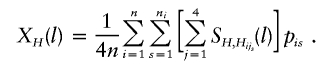
Suppose that n nuclear families are sampled with ti children in the ith family and that L tightly linked markers are typed both for the children and for the parents. Let yik denote the trait value of the kth child in the ith family. For a qualitative trait of interest, we let y=1 denote the affected individual and y=0 denote the unaffected individual. Our proposed method is based on the similarities of the haplotypes. First, we define the similarity between a pair of haplotypes around a specific marker. SHi,Hj(l), a natural measure of the similarity between two haplotypes Hi and Hj around the lth marker, is the length of the contiguous region around the lth marker over which the two haplotypes are identical by state (IBS). This similarity has also been used by Clayton and Jones (1999) and Bourgain et al. (2000, 2001, 2002), among others. For any pair of haplotypes Hi and Hj, the calculation of SHi,Hj(l), the similarity of the two haplotypes around the lth marker, is as follows. As illustrated in figure 1, starting from the lth marker, the marker alleles at that marker are compared between the two haplotypes. If the two alleles at the lth marker are not the same, then SHi,Hj(l)=0. If the two alleles at the lth marker are IBS, then the comparison is repeated for the right and left adjacent markers, as long as the alleles are IBS. SHi,Hj(l) is the distance between the leftmost and the rightmost markers with identical alleles. From this definition, SHi,Hj(l)=0 if the two haplotypes are not IBS at the lth marker or if the two haplotypes are IBS at the lth marker but not at the adjacent markers. Using the haplotype similarity between a pair of haplotypes, we define a haplotype-sharing score of a haplotype by comparing the haplotype with all of the 4n parental haplotypes. For any haplotype H, the haplotype-sharing score at the lth marker, denoted by XH(l), is defined as the average similarity between H and all of the 4n parental haplotypes:
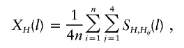 |
where Hi1,…,Hi4 denote the four parental haplotypes in the ith family. For the ith family, let Xi1(l),…,Xi4(l) denote the haplotype-sharing scores of the four parental haplotypes at the lth marker and let ξijk indicate whether the parental haplotype Hij is transmitted to the kth child—that is, ξijk=1 if Hij is transmitted to the kth child, and ξijk=-1 otherwise.
Figure 1.

Calculation of the similarity between two haplotypes around a specific marker. The similarity is taken as the length of the region shared IBS around this marker.
Some understanding of the nature of the haplotype-sharing score is given by considering the situation in which the similarity takes only two values η and 0, where η is the length of the chromosome region across all of the L markers (two haplotypes are IBS at all of the L markers). This situation means that, for any pair of haplotypes, either the marker alleles are identical across all of the L markers or there are no any adjacent markers at which the marker alleles are IBS. If the lth marker is either at or tightly linked with the disease-susceptibility locus, then, at the lth marker, the similarity of two haplotypes both of which have the disease mutation is expected to be larger than the similarity of two haplotypes both of which do not have the disease mutation or one of which has the disease mutation and the other of which does not have the disease mutation. Assume that the similarity of two haplotypes is η if both two haplotypes bear the disease mutation and is 0 otherwise. Suppose that, among the 4n parental haplotypes, there are m haplotypes with the disease mutation. Under these circumstances, the haplotype-sharing score will be  for a haplotype with the disease mutation and will be 0 otherwise. In general, we would expect the haplotype-sharing score to be larger for a haplotype with the disease mutation than that for a haplotype without the disease mutation.
Consider a disease-susceptibility locus with two alleles D and d, each with a population frequency pD and 1-pD, respectively. Here, “no linkage” means that there is no linkage between the disease-susceptibility locus and any one of the L markers considered; “no association” means that, for any haplotype H across the L markers, P(DH)=pDpH, where pH is the population frequency of haplotype H. The null hypothesis is no linkage or no association, whereas the alternative hypothesis is linkage and association. As noted by Monks and Kaplan (2000), the part of the hypothesis that concerns linkage is straightforward; however, the part that concerns association requires further details, because of the population stratification. If population stratification exists, then the null hypothesis is that there is no linkage or association in any of the subpopulations from which the parental chromosomes might originate. To illustrate our method, we begin with the case of known phase information, and we then describe how to extend our method to the case of ambiguous phase information.
Known Phase Information
We begin with the case for which the phase information is available. For the ith family and the lth marker, let  denote the difference of the haplotype-sharing scores between the parental haplotypes that are transmitted and the parental haplotypes that are not transmitted to the kth child. Under the null hypothesis, E(ξijk|children’s trait values and parental haplotypes) = 0; therefore,
  . One measure of the relationship between a chromosome region and the disease-susceptibility locus is the covariance between the trait values and a variable representing the transmission of the haplotypes across the chromosome region considered (Rabinowitz 1997; Monks and Kaplan 2000). Up to a constant, the estimated covariance between yij and xij(l) can be written as
  , where c is an arbitrary constant. The choice of c will be discussed later. As shown in appendix A, under the null hypothesis, the transmission of the haplotypes is independent of the trait value, and, thus,
  for any constant c.
To explain the nature of Ui(l), let us consider a nuclear family with one child. Assume that Hi1 and Hi3, among parental haplotypes Hi1,…,Hi4, are transmitted to the child. Then,
where Xij(l) is the haplotype-sharing score of Hij. Let c be the average trait value over all sampled children. If the disease mutation causes high trait values, then the high trait values will often occur with the transmission of haplotypes with the disease mutation; therefore,  is expected to be positive for the high trait value yi1(yi1-c⩾0). Thus, we would expect Ui(l) to be positive. Similarly, if the disease mutation causes low trait values, we would expect Ui(l) to be negative. Thus, it is reasonable to construct a test of linkage and association on the basis of Ui(l).
Let  , where wi>0 is a constant. Our HS-TDT test statistic is defined by
  . If we know that the disease mutation causes high (low) trait values, then we can let
  (
( ). For a qualitative trait of interest, if we assign a trait value 1 for the affected individuals and a trait value 0 for the unaffected individuals, then we can let
  . Certainly, the power of the test will be different for different values of wi and c. For the case of a single marker, Sun et al. (2000), Rabinowitz (1997), and Monks and Kaplan (2000) constructed tests of similar form. Monks and Kaplan (2000) used wi=1/ti in their test; Sun et al. (2000) and Rabinowitz (1997) used wi=1, which gives larger weight to the family with more children. In our simulations, we use wi=1/ti. Further investigation is needed for choosing optimal weights. For the choice of c, in most cases, we let
 |
be the mean trait value over all children in all of the families. When the trait value is qualitative and only affected children and their parents are sampled, we let c=0.
As shown in appendix B, for a qualitative trait, if all of the children are affected and wi=1, then the test statistic U is the same as the MILC method of Bourgain et al. (2000).
To evaluate the p value of the test, we use a permutation procedure. Under the null hypothesis, a parent is equally likely to transmit one of the two haplotypes. If there is only one child, the permutation procedure can be based on a random assignment of one of the two paternal haplotypes and one of the two maternal haplotypes as the transmitted haplotypes. For the case of more than one child, as noted by Monks and Kaplan (2000), complications arise in the presence of linkage. In this case, children with shared haplotypes will have similar trait values, even in the absence of association. For the families with more than one child, we use the method proposed by Monks and Kaplan (2000)—that is, we simultaneously permute the transmitted and nontransmitted status of the parental haplotypes for all of the children in the family. This procedure is equivalent to multiplying the value of Ui(l) by di, where di=1 or −1 with equal probability.
Ambiguous Phase Information
The method proposed in the previous subsection assumes that the haplotypes of both parents and children are known. However, for data collected on nuclear families, the haplotypes may not be uniquely determined. For a nuclear family with one child, necessary conditions for the haplotype ambiguity include that there is a locus at which both of the parents and their offspring have the same heterozygous genotype and that there is another locus at which both of the parents and their offspring do not have the same homozygous genotype (Dudbridge et al. 2000). Unless there is complete disequilibrium among the markers, the proportion of ambiguous families increases with the number of markers studied.
Bourgain et al. (2002) proposed a method to deal with the ambiguity of the haplotypes. In their approach, transmitted and nontransmitted haplotypes were reconstructed from the genotypes of the parents and the offspring. Alleles at loci where the phases could not be unambiguously determined were treated as missing alleles. In computing the similarity between two haplotypes, this approach either considered the missing allele as a different allele or discarded the marker with missing alleles. For the tightly linked markers considered in the present article, we propose the following method to deal with the ambiguity of the haplotypes.
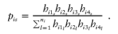
For a family with ambiguous haplotypes, let g denote the set of the observed multimarker genotypes of the family members. Suppose that the haplotype groups  and s=1,…,sg are all of the possible parental-haplotype groups that are compatible with g and let his denote the frequency of haplotype His. If m∈{1,…,sg} such that
 |
then we assign H1m,H2m,H3m,H4m as the four parental haplotypes of this ambiguous family. Under the assumption of Hardy-Weinberg equilibrium, the above procedure is to assign to each ambiguous family its most likely haplotype group. After assigning the parental haplotypes to each ambiguous family, the HS-TDT (described in the previous subsection [“Known Phase Information”]) can be performed as if we knew the haplotypes for each family.
For an arbitrary set of haplotype frequencies, we have proved in appendix C that, under the null hypothesis, E(ξijk|the children’s trait values and the parental genotypes) = 0 and, thus, that  . Because
  under the null hypothesis, regardless of the choice of the haplotype frequencies, a particular choice of the haplotype frequencies affects only the power, but not the validity, of our HS-TDT.
In the present article, the haplotype frequencies are estimated by treating all parents as a random sample of unrelated individuals from a population with Hardy-Weinberg equilibrium. The maximum-likelihood estimates of haplotype frequencies under the constraints of family information can be obtained by the expectation-maximization algorithm (Rohde and Fuerst 2001; Chen and Zhang 2003).
As an alternative method to treat the ambiguous phase, we can also use the estimated haplotype frequencies to construct the test statistic similar to that of Zhao et al. (2000). In brief, suppose that  and s=1,…,ni are all of the possible parental-haplotype groups that are compatible with the genotype set of the ith family and let hijs denote the frequency of haplotype Hijs. Define
 |
For a haplotype H, the haplotype-sharing score at the lth marker can be defined as
 |
Let Xi1s(l), Xi2s(l), Xi3s(l), and Xi4s(l) denote the haplotype-sharing scores of the sth possible parental-haplotype group of the ith family. Then, xik(l) can be defined as
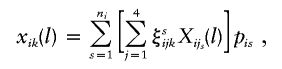 |
where ξsijk indicates whether the parental haplotype Hijs is transmitted to the kth child; ξsijk=1 if Hijs is transmitted to the kth child, and ξsijk=-1 otherwise. Now, we can construct the HS-TDT test statistic by using the same formulas given in the previous subsection (“Known Phase Information”); however, our simulations show that the HS-TDT has a very similar power to HS-TDT1, which assumes that the parental haplotypes are known. Thus, using haplotype frequencies instead to assign the most likely haplotype group to each family may have little benefit; however, using the haplotype frequencies to construct the test statistic may lead to extra computational burdens.
Simulation Setup
We evaluate the performance of our method through simulation studies. We consider 11 biallelic markers that are evenly distributed across a 1-cM region. The disease-susceptibility locus has two alleles, D and d.
Data Sets for Assessment of Type I Error
To assess the type I error rate and the robustness to the population stratification of our proposed method, we consider a stratified population that consists of two subpopulations. For the first subpopulation, the two alleles at each marker have equal allele frequencies, and the frequency of allele D at the disease locus is pD=0.2; for the second subpopulation, we assume that the minor allele at each marker has an allele frequency of q2, we vary q2 from 0.1 to 0.5, and the frequency of allele D at the disease locus is pD=0.3. We assume that the distance between the disease locus and the first marker is 10 cM. Furthermore, we assume that there is neither association between the disease locus and the marker region nor association among the 11 markers within each subpopulation. To generate the haplotypes in the two subpopulations, we generate alleles in each marker and the disease locus independently, according to the allele frequencies within each subpopulation.
For a qualitative trait of interest, we sample nuclear families with one affected child. We randomly choose a family with one child, and we use the acceptance and rejection method to decide whether we accept this family—that is, we accept the family with probabilities P(affected|DD), P(affected|Dd), and P(affected|dd) for the child’s genotypes DD, Dd, and dd, respectively. To generate a randomly sampled family, we generate the parental genotypes by drawing haplotypes in the following way: with probability pD, we draw a haplotype with a disease mutation D; otherwise, we draw a normal haplotype, and each of the parents then randomly transmits one of the two haplotypes to the child by considering the possible recombinations between the disease-susceptibility locus and the marker region but ignoring the recombinations among the 11 markers. Let f11 = P(affected|DD), f12 = P(affected|Dd), and f22 = P(affected|dd) be the penetrances; in our simulations, we assume that f11, f12, and f22 are 0.3, 0.16, and 0.02, respectively, in the first subpopulation, and 0.2, 0.11, and 0.02, respectively, in the second subpopulation. Let pp be the proportion of families sampled from the first subpopulation; we consider pp to be 1/2, 1/4, and 1/6 in our simulations.
For a quantitative trait of interest, half of the families that we sample are from the first subpopulation, and the other half are from the second subpopulation. Let yij be the trait value of the jth child in the ith family. We generate the trait value by using the model y=μ(1+x1)+e, where x1 denotes the additive genotypic score (with x1 being 1, 0, and −1 for genotypes DD, Dd, and dd, respectively) and e is a standard normal random variable. If a family comes from the first subpopulation, then μ=2; otherwise, μ=4.
Data Sets for Assessment of Power
To assess power, the haplotypes are obtained using a method similar to that described by Tzeng et al. (2003) and Lam et al. (2000). This method mimics features of natural populations as closely as possible by using a direct simulation method. Diploid individuals are paired at random in their generation and are mated. The number of children per couple is randomly drawn from a Poisson distribution with mean λ. Each population is founded by 100 individuals, and the expected size remains at 100 for 50 generations (the reproduction rate λ=2). This initialization, together with small population growth in early generations, generates random linkage disequilibrium among alleles on normal chromosomes. After 50 generations, the population grows exponentially for 100 generations, to a final size of 10,000 individuals; during this period, the reproduction rate λ is determined by the exponential growth rate. We consider two scenarios: one ancestral haplotype and two ancestral haplotypes. For the first scenario, one disease mutation is introduced on one chromosome in the 51st generation; for the second scenario, two disease mutations are introduced in the 51st and 61st generations, respectively. To mimic the common disease, we choose only the populations in which the relative frequency of disease mutation is no less than 0.1. For computational simplicity, we reinitiate the simulation if the relative frequency of disease mutation is <0.1 in the 70th generation.
We simulate 11 biallelic markers, covering a 1-cM region, with spacing of 0.1 cM between the adjacent markers. The sixth marker is located at the disease-susceptibility locus (assuming a negligible recombination rate), but the sixth marker is not the disease-susceptibility locus itself (i.e., the marker is not the functional polymorphism). We assume no mutation for the alleles at the 11 markers.
To generate the chromosome in the founder population, we generate alleles at each of the 11 markers independently, according to the allele frequencies. The minor allele frequency at each marker is drawn from a uniform distribution over the interval 0.1–0.4.
The simulation program produces populations from which samples of haplotypes with or without the disease mutation can be drawn. For a qualitative trait of interest, to compare our test with that proposed by Zhao et al. (2000), we consider the nuclear families with one affected child (Zhao et al.’s test can consider only one affected child). Let RR denote the relative risk of genotypes DD to dd and let qD denote the frequency of allele D. For the given RR, qD, and disease model, the parental genotypes at the disease-susceptibility locus are generated according to the probability of mating types, under the condition that the child is affected. The parental multimarker genotypes are generated according to the genotypes at the disease-susceptibility locus; for example, if the father’s genotype at the disease-susceptibility locus is Dd, then we randomly choose one haplotype with the disease mutation and one haplotype without the disease mutation, to form the father’s multimarker genotype. Conditional on the parents’ mating types, the affected child’s genotype is generated by ignoring the recombination. In our simulations, we set qD=0.3, vary RR from 2 to 5, and consider three disease models—recessive, additive, and dominant.
For the case of the quantitative trait, we use a random sampling scheme. Each parental genotype is generated by drawing a haplotype bearing the disease mutation with probability pD and a normal haplotype with probability 1-pD. Each of the parents randomly transmits one of the two haplotypes to form their child’s genotype. The trait values of the children are generated by the model y=μ(x1+βx2)+e, where x1 denotes the additive genotypic score (with x1 being 1, 0, and −1 for genotypes DD, Dd, and dd, respectively), x2 denotes the dominant genotypic score (with x2 being 0, 1, and 0 for genotypes DD, Dd, and dd, respectively), β denotes the disease model (with β being −1, 0, and 1 for recessive, additive, and dominant models, respectively), and e is a standard normal variable. The value of μ can be calculated from the value of heritability. In our simulations, we set qD=0.3, vary the values of heritability from 4% to 10%, and vary the number of children from 1 to 5.
Results
For each simulation scenario, 1,000 independent samples (100 populations with 10 samples from each population for power comparisons) of 200 nuclear families were generated in the studies of the type I error rate and the power. For each sample, the p values of all of the tests considered were estimated by 1,000 permutations.
Type I Error Rate
We first verified that the HS-TDT had the correct nominal type I error rate in a structured population. To see how the ambiguous phase affects the type I error rate, we also gave the estimated type I error rate of HS-TDT1, which is the HS-TDT under the assumption that the phase information is known. For 1,000 replicated samples, the SEs for the type I error rate were  and
and  , for the nominal levels of 0.05 and 0.01, respectively. The 95% CIs were 0.0362–0.0638 and 0.0037–0.0163, respectively. The estimated type I errors of the two tests, HS-TDT1 and HS-TDT, are summarized in table 1, for a qualitative trait, and in table 2, for a quantitative trait. It is easy to see that the estimated type I errors of the two tests are not statistically significantly different from the nominal levels. For the cases when the frequency of the minor allele is 0.5 at each of the two subpopulations, there are a large number of possible haplotypes, and, therefore, almost all of the haplotypes are rare. In this case, the error rate of resolving the ambiguous haplotypes is >20% (results not shown); however, the HS-TDT still has the correct type I error rate.
Table 1.
Type I Error Rates of the Tests, HS-TDT and HS-TDT1—for a Qualitative Trait[Note]
|
Type I Error Rate at |
||||
| Significance Level .05, for |
Significance Level .01, for |
|||
| Parameters | HS-TDT1 | HS-TDT | HS-TDT1 | HS-TDT |
| Sample size 100: | ||||
| q2=.1: | ||||
| pp=1/2 | .047 | .05 | .01 | .011 |
| pp=1/4 | .05 | .045 | .009 | .008 |
| pp=1/6 | .052 | .058 | .011 | .009 |
| q2=.3: | ||||
| pp=1/2 | .056 | .061 | .015 | .011 |
| pp=1/4 | .05 | .052 | .013 | .014 |
| pp=1/6 | .047 | .045 | .007 | .005 |
| q2=.5: | ||||
| pp=1/2 | .052 | .042 | .014 | .009 |
| pp=1/4 | .054 | .05 | .011 | .015 |
| pp=1/6 | .057 | .049 | .011 | .015 |
| Sample size 200: | ||||
| q2=.1: | ||||
| pp=1/2 | .053 | .051 | .012 | .009 |
| pp=1/4 | .052 | .055 | .012 | .011 |
| pp=1/6 | .058 | .057 | .015 | .015 |
| q2=.3: | ||||
| pp=1/2 | .054 | .062 | .013 | .013 |
| pp=1/4 | .065 | .062 | .017 | .016 |
| pp=1/6 | .045 | .049 | .009 | .008 |
| q2=.5: | ||||
| pp=1/2 | .036 | .042 | .007 | .009 |
| pp=1/4 | .054 | .046 | .015 | .009 |
| pp=1/6 | .063 | .059 | .01 | .011 |
Note.— The sample size is the number of nuclear families. The minor allele frequency in the second subpopulation is denoted by q2. pp denotes the proportion of the sample from the first subpopulation.
Table 2.
Type I Error Rates of the Two Tests, HS-TDT and HS-TDT1—for a Quantitative Trait[Note]
|
Type I Error Rate at |
||||
| Significance Level .05, for |
Significance Level .01, for |
|||
| Parameters | HS-TDT1 | HS-TDT | HS-TDT1 | HS-TDT |
| Sample size 100: | ||||
| q2=.1: | ||||
| nc=1 | .048 | .047 | .014 | .012 |
| nc=3 | .053 | .052 | .008 | .011 |
| nc=5 | .045 | .047 | .006 | .008 |
| q2=.3: | ||||
| nc=1 | .057 | .049 | .017 | .014 |
| nc=3 | .056 | .055 | .016 | .013 |
| nc=5 | .03 | .032 | .004 | .002 |
| q2=.5: | ||||
| nc=1 | .05 | .055 | .008 | .01 |
| nc=3 | .058 | .054 | .015 | .016 |
| nc=5 | .047 | .043 | .011 | .01 |
| Sample size 200: | ||||
| q2=.1: | ||||
| nc=1 | .051 | .049 | .016 | .013 |
| nc=3 | .049 | .052 | .01 | .009 |
| nc=5 | .067 | .061 | .018 | .016 |
| q2=.3: | ||||
| nc=1 | .067 | .066 | .015 | .018 |
| nc=3 | .062 | .062 | .013 | .013 |
| nc=5 | .054 | .055 | .013 | .012 |
| q2=.5: | ||||
| nc=1 | .048 | .045 | .011 | .008 |
| nc=3 | .044 | .057 | .017 | .014 |
| nc=5 | .071 | .069 | .014 | .012 |
Note.— The sample size is the number of nuclear families. The minor allele frequency in the second subpopulation is denoted by q2. The number of children in each family is denoted by “nc.”
Power Comparisons
Here, we describe the results from our power studies. The significance level was set at 0.05. The tests used for the comparisons are summarized in table 3. The powers of the single-marker methods, TDT and QTDT, are the powers of testing the sixth marker, which is the nearest to the disease-susceptibility locus (negligible recombination rate). The powers of the tests TDT2, TDT3, and TDT4 are the powers of the tests proposed by Zhao et al. (2000), using two, three, and four markers, respectively, around the susceptibility locus. In our simulation, 200 families were sampled. The numbers of distinct haplotypes varied from 35 to 55 in our simulated samples. On average, there were 13 common haplotypes (frequency ⩾0.01), which accounted for >90% of the total 800 haplotypes.
Table 3.
Test Statistics Compared
| Test Statistic | Details |
| HS-TDT | Haplotype-sharing TDT proposed in the present article |
| HS-TDT1 | Same as HS-TDT but assuming that the haplotype information is known |
| QTDT | Test proposed by Monks and Kaplan (2000) |
| TDT | Test proposed by Spielman et al. (1993) |
| TDT2, TDT3, and TDT4 | Tests proposed by Zhao et al. (2000) for tightly linked markers, using two, three, and four markers, respectively; haplotype frequencies were estimated by the EM algorithm by assuming Hardy-Weinberg equilibrium in the population under study |
For the case of a qualitative trait of interest, 200 families were ascertained through an affected child. On average, 35% of the families had ambiguous haplotypes. When the EM algorithm was used to reconstruct the haplotypes, the error rates varied from 0.5% to 5%. The power comparisons of the six tests—HS-TDT1, HS-TDT, TDT, TDT2, TDT3, and TDT4—are given in figure 2. We can see from the figure that the powers of HS-TDT1 and HS-TDT are very similar. One explanation may be that the error rate of haplotype reconstruction is not large; another may be that the true haplotype and the estimated haplotype, though different, have similar haplotype-sharing scores. The power comparisons show a similar pattern for different disease models. For all of the cases, the powers of both HS-TDT1 and HS-TDT are higher than the powers of the other four tests; of the four other tests, TDT2 has highest power for the case of one ancestral haplotype, and TDT3 has the highest power for the case of two ancestral haplotypes. In comparison with other tests, the performance of the single-marker TDT in the case of two ancestral haplotypes is not as good as that in the case of one ancestral haplotype.
Figure 2.

Power comparison of the six tests for a qualitative trait. The sample size is 200 families with one affected child in each family.
For a quantitative trait of interest, 200 families were randomly sampled. The powers of the three tests HS-TDT1, HS-TDT, and QTDT were compared. We present the power comparisons in figures 3 and 4. In figure 3, we summarize the power comparisons for different values of heritability with two children in each family; the power comparisons for a different number of children are given in figure 4. When there is only one child in each family, HS-TDT is slightly less powerful than HS-TDT1; when the number of children in each family is more than one, the powers of the HS-TDT and HS-TDT1 are very similar. In all of the cases, both HS-TDT and HS-TDT1 are more powerful than QTDT.
Figure 3.

Power comparison of the three tests for a quantitative trait—with two children in each family. The sample size is 200 families.
Figure 4.

Power comparison of the three tests for a quantitative trait—with heritability fixed at 6%. The sample size is 200 families.
We also performed another set of the simulations, in which the fourth marker was at the disease-susceptibility locus (which was not at the middle of the marker region). The power comparisons showed a similar pattern (results not shown).
Discussion
The TDT, proposed by Spielman et al. (1993), has proved to be a powerful approach. The TDT using multiple tightly linked markers may further increase the statistical power; however, in extending the single-marker TDT to the case of multiple tightly linked markers, we may encounter some difficulties: first, if we consider each haplotype as an allele and use the conventional single-marker TDT, then the rapid increase in the number of haplotypes with an increasing number of markers leads to low power for the conventional statistical tests; second, the parental haplotypes may not always be unambiguously reconstructed. In the present article, we have proposed the HS-TDT, a haplotype-based TDT using multiple tightly linked markers, to test linkage or association between the disease-susceptibility locus and a chromosome region in which several tightly linked markers have been typed. This method is applicable to both qualitative traits and quantitative traits. It is applicable to any size of nuclear family, with or without ambiguous phase information, and is applicable to any number of alleles at the markers considered. The degrees of freedom (in a broad sense) of the test increase linearly with the number of markers considered, rather than with the number of alleles at the markers. Our simulation results show that the HS-TDT has the correct type I error rate in structured populations and that the power of HS-TDT is higher than the power of the other methods.
In the present article, we have assumed that both parents were available for genotyping. In the case of a single marker, the TDT has been extended to the families consisting of siblings without parents (Curtis 1997; Boehnke and Langefeld 1998; Horvath and Laird 1998; Spielman and Ewens 1998; Teng and Risch 1999; Monks and Kaplan 2000) and to the families consisting of one child and one parent (Sun et al. 1999, 2000). Our method may be extended to both the case of siblings without parents and the case of siblings with only one parent. The other assumption made by our method is that there is no recombination among the tightly linked markers under study. This assumption can be relaxed to allow recombination among the markers, but more parameters are needed to define the recombination fractions among the markers; this, in turn, requires additional computation. Overall, there may be little benefit in considering the recombination for tightly linked markers. If linkage disequilibrium exists across the region for a nonadmixture population, then the recombination must be quite infrequent and probably can be safely ignored. For the admixture populations or founder populations, the recombination may be common among the markers with linkage disequilibrium. In that case, the method proposed by Bourgain et al. (2002) may be used to resolve the ambiguous haplotypes.
As stated above (see the “Results” section [“Power Comparisons”]), there may be two reasons for the similar powers of HS-TDT and HS-TDT1. One reason is that the error rate of haplotype reconstruction is small, especially for the case of a restricted number of haplotypes in the sample. As indicated by Chen and Zhang (2003), the error rate of haplotype reconstruction can be greatly improved if the parental genotypes are included. Another reason is that, even if the true haplotype and the estimated haplotype are different, the haplotype-sharing scores of the two haplotypes may be similar. Let us consider an ideal case, in which the haplotype-sharing score is 1 for the haplotypes with the disease mutation and is 0 otherwise. In this case, if the estimated haplotype H is different from the true haplotype H′ but H and H′ both bear the disease mutation or both do not bear the disease mutation, then the haplotype-sharing scores of H and H′ will be the same, and this kind of incorrect reconstruction of the haplotypes will not affect the power of the our test. In fact, we have done another set of simulations for power comparisons. In that set of simulations, we assumed that there was no association among the markers in the population at large and, thus, that the number of haplotypes was very large. In this case, the error rate of the haplotype reconstruction was large (15%–35%), but the powers of HS-TDT and HS-TDT1 were still very similar. The reason is that almost all of the haplotypes that could not be correctly reconstructed were rare haplotypes without the disease mutation, and the rare haplotypes without the disease mutation had similar haplotype-sharing scores.
In our simulation studies, we assumed that there were either one or two ancestral haplotypes. For the case of no ancestral haplotypes, the performance of the HS-TDT and the power comparisons will need further investigation.
Acknowledgments
This work was supported, in part, by the Research Excellence Fund grant of Michigan Technological University and the National Natural Science Foundation grant (10071011) of China. We thank Dr. Francoise Clerget-Darpoux and Dr. Catherine Bourgain for their constructive comments on the manuscript.
Appendix A : Expectation of U(l) under the Null Hypothesis for Known Phase Information
If there is no linkage between the disease-susceptibility locus and the chromosome region considered, then it is obvious that the parents will transmit each of the two haplotypes to the child with equal probability, regardless of the child’s trait value. Thus, E(ξijk|child's trait, parents' genotype) = 0, and  . In the following discussion, we assume that there is no association but that there may be linkage.
First, assume that the families are sampled from a homogeneous population with Hardy-Weinberg equilibrium both at the chromosome region considered and at the disease-susceptibility locus. Let D1 and D2 denote the two alleles at the disease-susceptibility locus. For an individual from this population, let Y and g respectively denote this individual’s trait value and multimarker genotype across all of the markers considered. Then, for any y,
Denote the two haplotypes of g by H1 and H2. Under the assumption of Hardy-Weinberg equilibrium and no association, we have
 |
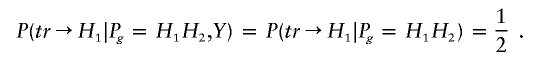
From equations (A1) and (A2), it follows that P(Y⩽y,g)=P(Y⩽y)P(g). This means that the trait value and the genotype are independent. Let Pg denote the genotype of one parent, let tr→Hi denote that the haplotype Hi has been transmitted to the child, and let Y denote the trait value of the child. Then, given the child’s trait value, the probability of one parent with haplotypes H1 and H2 transmitting H1 is
 |
Thus, E(ξijk|Y, parental genotypes) = 0, and  . Furthermore,
  .
.
Consider a population that is composed of m subpopulations with Hardy-Weinberg equilibrium within each subpopulation. Note that the large population may not have Hardy-Weinberg equilibrium. Given the child’s trait value, the probability that one parent with haplotypes H1 and H2 transmits H1 is
 |
Using an argument similar to the case of homogeneous population with Hardy-Weinberg equilibrium, we can conclude that  .
.
Appendix B : The MILC Method of Bourgain et al. Is a Special Case of HS-TDT
We will show that, for the case of qualitative traits, if all of the children are affected and wi=1, then the HS-TDT will be the MILC method proposed by Bourgain et al. (2000). Without loss of generality, we assume that there is one affected child in each family. For the ith family, let Hi1 and Hi2 be the paternal haplotypes and Hi3 and Hi4 be the maternal haplotypes and let Hi1 and Hi3 be transmitted to the child. Then, the HS-TDT statistic is
Note that, for any two haplotypes H1 and H2, SH1,H2=SH2,H1, and SH1,H1=SH2,H2. We have
 |
Denoting Hi=Hi1, Hi+n=Hi3, H*i=Hi2, and H*i+n=Hi4, for i=1,2,…,n, we obtain
 |
where MT(l) and Mn(l) are the mean similarities of all possible pairs of haplotypes in the transmitted group and in the nontransmitted group, respectively. The test statistic of the MILC method of Bourgain et al. (2000) is
which is equal to our test statistic U up to a constant  . Therefore, the two tests are equivalent.
Appendix C : The Case of Ambiguous Haplotypes,  , Regardless of the Haplotype Frequencies
For clarity of presentation, we assume that there is one child in each nuclear family. In the discussion that follows, we designate {ij,kl} as a haplotype group in which the father has haplotypes Hi and Hj and transmits Hi to the child and in which the mother has haplotypes Hk and Hl and transmits Hk to the child. Let Pij,kl be the conditional probability that the father has haplotypes {Hi,Hj} and transmits Hi to the child and that the mother has haplotypes {Hk,Hl} and transmits Hk to the child, given that the child’s trait value is Y.
From appendix A, we know that, under the null hypothesis, Pij,kl=Pji,lk. For a family with ambiguous haplotypes, let Go and Gp denote the observed multimarker genotypes of the child and the parents, respectively. Let {1s2s,3s4s}, s=1,…,sg, be the all possible haplotype groups that are compatible with the set of genotypes {Go,Gp}. Choosing an arbitrary s, let G′o denote the genotype corresponding to haplotype {H2s,H4s}. Then, for every {1s2s,3s4s} compatible with the genotype set {Go,Gp}, the set {2s1s,4s3s} must be compatible with {G′o,Gp}. Thus, under the null hypothesis, the probabilities of Go and G′o are the same given the parental genotype Gp and the child’s trait value Y—that is,
 |
where Y and Y′ denote the trait values of the children with genotypes Go and G′o, respectively.
For an arbitrary set of haplotype frequencies his, suppose that
 |
Then, the haplotype group {1m2m,3m4m} will be assigned to the family {Go,Gp}, and the haplotype group {2m1m,4m3m} will be assigned to the family {G′o,Gp}. Let ξi indicate whether the parental haplotype Him(i=1,2,3,4) is transmitted to the child; ξi=1 if Him is transmitted to the child, and ξi=-1 otherwise. Note that ξ2=-ξ1 and ξ4=-ξ3. In the discussion that follows, we assume the null hypothesis to be true. Let P▵ denote the conditional probability given the parents genotypes and the child’s trait value. We have
Similarly, we can prove that
It follows from equations (C1) and (C2) that P▵(ξ1=1)=P▵(ξ1=-1)=1/2. Thus, the expectation of Ui(l) is 0, and the expectation of U(l) is also 0.
Appendix D : Degrees of Freedom in a Broad Sense
The test statistic of HS-TDT is  , which is equivalent to
  . For the large sample size, U(l) will be approximately normally distributed. Thus, if U(1),…,U(L) are independent, then
  will have a χ2 distribution, with degrees of freedom equaling L (the number of markers). Since our test statistic is equivalent to using the maximum of U2(l), instead of the sum of U2(l), and since U(1),…,U(L) may be dependent, we say that the degrees of freedom of our test are equal to L in a broad sense. The broad sense of degrees of freedom in the MILC method proposed by Bourgain et al. (2000) has the same meaning.
References
- Allison DB (1997) Transmission-disequilibrium tests for quantitative traits. Am J Hum Genet 60:676–690 (erratum 60:1571) [PMC free article] [PubMed] [Google Scholar]
- Bickeboller H, Clerget-Darpoux F (1995) Statistical properties of the allelic and genotypic transmission/disequilibrium test for multiallelic markers. Genet Epidemiol 12:865–870 [DOI] [PubMed] [Google Scholar]
- Boehnke M, Langefeld CD (1998) Genetic association mapping based on discordant sib pairs: the discordant-alleles test. Am J Hum Genet 62:950–961 [DOI] [PMC free article] [PubMed] [Google Scholar]
- Bourgain C, Génin E, Holopainen P, Mustalahti K, Mäki M, Partanen J, Clerget-Darpoux F (2001) Use of closely related affected individuals for the genetic study of complex disease in founder populations. Am J Hum Genet 68:154–159 [DOI] [PMC free article] [PubMed] [Google Scholar]
- Bourgain C, Genin E, Ober C, Clerget-Darpoux F (2002) Missing data in haplotype analysis: a study on the MILC method. Ann Hum Genet 66:99–108 [DOI] [PubMed] [Google Scholar]
- Bourgain C, Genin E, Quesneville H, Clerget-Darpoux F (2000) Search for multifactorial genes in founder populations. Ann Hum Genet 64:255–265 [DOI] [PubMed] [Google Scholar]
- Chen HS, Zhang SL (2003) Haplotype inference for multiple tightly linked marker phenotypes including nuclear family information. In: Valafar F, Valafar H (eds) Proceeding of the International Conference on Mathematics and Engineering Techniques in Medicine and Biological Sciences. CSREA Press, Las Vegas, pp 165–171 [Google Scholar]
- Clayton DG (1999) A generalization of the transmission/disequilibrium test for uncertain-haplotype transmission. Am J Hum Genet 65:1170–1177 [DOI] [PMC free article] [PubMed] [Google Scholar]
- Clayton DG, Jones H (1999) Transmission/disequilibrium tests for extended marker haplotypes. Am J Hum Genet 65:1161–1169 [DOI] [PMC free article] [PubMed] [Google Scholar]
- Curtis D (1997) Use of siblings as control in case-control association studies. Ann Hum Genet 61:319–333 [DOI] [PubMed] [Google Scholar]
- Dudbridge F, Koeleman BP, Todd JA, Clayton DG (2000) Unbiased application of the transmission/disequilibrium test to multilocus haplotypes. Am J Hum Genet 66:2009–2012 [DOI] [PMC free article] [PubMed] [Google Scholar]
- Horvath S, Laird NM (1998) A discordant-sibship test for disequilibrium and linkage: no need for parental data. Am J Hum Genet 63:1886–1897 [DOI] [PMC free article] [PubMed] [Google Scholar]
- Knapp M (1999) The transmission/disequilibrium test and parental-genotype reconstruction: the reconstruction combined disequilibrium test. Am J Hum Genet 64:861–870 [DOI] [PMC free article] [PubMed] [Google Scholar]
- Lam JC, Roeder K, Devlin B (2000) Haplotype fine mapping by evolutionary trees. Am J Hum Genet 66:659–673 [DOI] [PMC free article] [PubMed] [Google Scholar]
- Lazzeroni LC, Lange K (1998) A conditional inference framework for extending the transmission/disequilibrium test. Hum Hered 48:67–81 [DOI] [PubMed] [Google Scholar]
- Li J, Wang D, Dong J, Jiang R, Zhang K, Zhang S, Zhao H, Sun F (2001) The power of transmission disequilibrium tests for quantitative traits. Genet Epidemiol 21 Suppl 1:S632–S637 [DOI] [PubMed] [Google Scholar]
- Merriman TR, Eaves IA, Twells RC, Merriman ME, Danoy PA, Muxworthy CE, Hunter KM, Cox RD, Cucca F, McKinney PA, Shield JP, Baum JD, Tuomilehto J, Tuomilehto-Wolf E, Ionesco-Tirgoviste C, Joner G, Thorsby E, Undlien DE, Pociot F, Nerup J, Rønningen KS, Bain SC, Todd JA (1998) Transmission of haplotypes of microsatellite markers rather than single marker alleles in the mapping of a putative type 1 diabetes susceptibility gene (IDDM6). Hum Mol Genet 7:517–524 [DOI] [PubMed] [Google Scholar]
- Monks SA, Kaplan NL (2000) Removing the sample restrictions from family-based test of association for quantitative-trait locus. Am J Hum Genet 66:576–592 [DOI] [PMC free article] [PubMed] [Google Scholar]
- Rabinowitz D (1997) A transmission disequilibrium test for quantitative trait loci. Hum Hered 47:342–350 [DOI] [PubMed] [Google Scholar]
- Rabinowitz D, Laird N (2000) A unified approach to adjusting association tests for population admixture with arbitrary pedigree structure and arbitrary missing marker information. Hum Hered 50:211–223 [DOI] [PubMed] [Google Scholar]
- Risch N, Merikangas K (1996) The future of genetic studies of complex human diseases. Science 273:1516–1517 [DOI] [PubMed] [Google Scholar]
- Rohde K, Fuerst R (2001) Haplotyping and estimation of haplotype frequencies for closely linked biallelic multilocus genetic phenotypes including nuclear family information. Hum Mutat 17:289–295 [DOI] [PubMed] [Google Scholar]
- Schaid DJ (1996) General score tests for associations of genetic markers with disease using cases and their parents. Genet Epidemiol 13:423–449 [DOI] [PubMed] [Google Scholar]
- Schaid DJ, Rowland CR (1998) The use of parents, sibs, and unrelated controls to detection of associations between genetic markers and disease. Am J Hum Genet 63:1492–1506 [DOI] [PMC free article] [PubMed] [Google Scholar]
- Seltman H, Roeder K, Devlin B (2001) Transmission/disequilibrium test meets measured haplotype analysis: family-based association analysis guided by evolution of haplotypes. Am J Hum Genet 68:1250–1263 [DOI] [PMC free article] [PubMed] [Google Scholar]
- Sham PC, Curtis D (1995) An extended transmission/disequilibrium test (TDT) for multi-allele marker loci. Ann Hum Genet 59:323–336 [DOI] [PubMed] [Google Scholar]
- Spielman RS, Ewens WJ (1998) A sibship test for linkage in the presence of association: the sib transmission/disequilibrium test. Am J Hum Genet 62:450-458 [DOI] [PMC free article] [PubMed] [Google Scholar]
- Spielman RS, McGinnis RE, Ewens WJ (1993) The transmission test for linkage disequilibrium: the insulin gene and insulin-dependent diabetes mellitus (IDDM). Am J Hum Genet 52:506–516 [PMC free article] [PubMed] [Google Scholar]
- Sun F, Flanders WD, Yang Q, Khoury MJ (1999) Transmission disequilibrium test (TDT) when only one parent is available: the 1-TDT. Am J Epidemiol 150:97–104 [DOI] [PubMed] [Google Scholar]
- Sun F, Flanders WD, Yang Q, Zhao H (2000) Transmission/disequilibrium tests for quantitative traits. Ann Hum Genet 64:555–565 [DOI] [PubMed] [Google Scholar]
- Teng J, Risch N (1999) The relative power of family-based and case-control designs for linkage disequilibrium studies of complex human diseases. II. Individual genotyping. Genome Res 9:234–241 [PubMed] [Google Scholar]
- Tzeng JY, Devlin B, Wasserman L, Roeder K (2003) On the identification of disease mutations by the analysis of haplotype similarity and goodness of fit. Am J Hum Genet 72:891–902 [DOI] [PMC free article] [PubMed] [Google Scholar]
- Zhao H, Zhang S, Merikangas KR, Trixler M, Wildenauer DB, Sun F, Kidd KK (2000) Transmission/disequilibrium test using multiple tightly linked markers. Am J Hum Genet 67:936–946 [DOI] [PMC free article] [PubMed] [Google Scholar]