

Abstract
We present the results of a simulation study that indicate that true haplotypes at multiple, tightly linked loci often provide little extra information for linkage-disequilibrium fine mapping, compared with the information provided by corresponding genotypes, provided that an appropriate statistical analysis method is used. In contrast, a two-stage approach to analyzing genotype data, in which haplotypes are inferred and then analyzed as if they were true haplotypes, can lead to a substantial loss of information. The study uses our COLDMAP software for fine mapping, which implements a Markov chain–Monte Carlo algorithm that is based on the shattered coalescent model of genetic heterogeneity at a disease locus. We applied COLDMAP to 100 replicate data sets simulated under each of 18 disease models. Each data set consists of haplotype pairs (diplotypes) for 20 SNPs typed at equal 50-kb intervals in a 950-kb candidate region that includes a single disease locus located at random. The data sets were analyzed in three formats: (1) as true haplotypes; (2) as haplotypes inferred from genotypes using an expectation-maximization algorithm; and (3) as unphased genotypes. On average, true haplotypes gave a 6% gain in efficiency compared with the unphased genotypes, whereas inferring haplotypes from genotypes led to a 20% loss of efficiency, where efficiency is defined in terms of root mean integrated square error of the location of the disease locus. Furthermore, treating inferred haplotypes as if they were true haplotypes leads to considerable overconfidence in estimates, with nominal 50% credibility intervals achieving, on average, only 19% coverage. We conclude that (1), given appropriate statistical analyses, the costs of directly measuring haplotypes will rarely be justified by a gain in the efficiency of fine mapping and that (2) a two-stage approach of inferring haplotypes followed by a haplotype-based analysis can be very inefficient for fine mapping, compared with an analysis based directly on the genotypes.
Introduction
Although haplotypes provide more information than the corresponding genotypes (since haplotypes equal genotypes plus phase information), the resulting gain in efficiency for linkage-disequilibrium (LD) fine mapping of disease-predisposing variants (see, e.g., Clayton 2000) has not hitherto been quantified. Indeed, until recently, there has been little multipoint, genotype-based statistical methodology available for fine mapping. Here, we demonstrate that, given appropriate statistical analyses, haplotypes at SNP markers may be only slightly more advantageous for fine mapping than the corresponding unphased genotypes.
The question is important because obtaining haplotypes directly in the laboratory is either infeasible or much more expensive than obtaining genotypes. Our results therefore suggest that, for fine mapping, the additional cost of obtaining direct haplotypes will rarely be justified. Instead, it will usually be more cost-effective to adopt multipoint, genotype-based statistical analyses with a slightly larger sample size than would be needed for directly measured haplotype data.
Lacking appropriate genotype-based methodology, many researchers have adopted a two-stage approach: a phase reconstruction software package, such as SNPHAP (SNPHAP Web site) or PHASE (Stephens et al. 2001; Stephens and Donnelly 2003), is employed to infer haplotypes, which are then treated as true haplotypes in a subsequent multipoint fine-mapping analysis. This two-stage approach is unsatisfactory because it is difficult to incorporate the uncertainty arising at the first stage into the subsequent multipoint mapping analysis and, hence, to produce a valid overall measure of confidence in any estimates obtained. Moreover, the methods employed to infer haplotypes do not take account of phenotypes, which are potentially informative about phase. Perhaps most importantly, errors in phase reconstruction tend to be consistent with the prevailing LD pattern, so the reconstructed data set tends to exaggerate the true level of LD, which can distort fine-mapping inferences. We show below that the loss of efficiency for fine mapping that results from the use of inferred haplotypes can be substantial, and, since our analyses based directly on unphased genotypes are relatively efficient, it is the two-stage approach that is responsible for most of the efficiency loss, not the lack of phase information inherent in genotype data.
Douglas et al. (2001) and Schaid (2002) have reported that estimating haplotype frequencies from genotype data leads to a substantial loss of efficiency compared with using directly measured haplotypes or those inferred from pedigrees. However, both studies considered only the estimation of haplotype frequencies, not fine mapping. Furthermore, their simulations did not employ a population-genetics model, and those of Douglas et al. (2001) assumed no LD and thus have little relevance to fine mapping.
Version 2 of our COLDMAP fine-mapping software handles genotype data. It is an extension of version 1, the haplotype-only algorithm described by Morris et al. (2002), and so retains the same modeling assumptions and Markov chain–Monte Carlo (MCMC) updates that are reviewed briefly below. In version 2, the unknown phases are treated as latent variables that are updated in the MCMC algorithm according to their joint probability under the model, in the same way as all other parameters. This carries a computational overhead of ∼50% compared with the use of haplotype data. Morris et al. (2003) described a successful application of COLDMAP (version 2) that identified a 185-kb interval within an 890-kb candidate region for CYP2D6, a known causal locus for the poor metabolizer phenotype (Hosking et al. 2002). The median estimate was ∼25 kb from the causal locus, and the algorithm correctly distinguished individuals homozygous for the major mutant allele from those carrying minor mutants.
In this study, we briefly review the modeling assumptions and MCMC algorithm of COLDMAP, version 1 (haplotypes-only version), and we describe the extension to handle genotype data incorporated in version 2. We then describe a simulation study involving 100 data sets for each of 18 disease models. Each data set consists of 100 cases and 100 controls typed at 20 SNP markers spanning a 950-kb region. To evaluate the efficiency for fine mapping, COLDMAP was applied to three different data formats: true haplotypes, haplotypes inferred from unphased genotypes using SNPHAP, and unphased genotypes. To illustrate the implications of the simulation results, we compare the results of our COLDMAP (version 2) analysis of unphased genotypes in the CYP2D6 data set with a version 1 analysis of haplotypes inferred using SNPHAP.
Methods
Consider a sample of unrelated affected cases and unaffected controls, typed at SNPs spanning a candidate region for a disease-predisposing locus. We denote the resulting phase-unknown genotypes by GA and GU in cases and controls, respectively; HA and HU represent the underlying haplotype pairs.
The goal is to approximate f(x|GA,GU), the posterior density of the location, x, of the disease locus, given the observed genotypes, which can be expressed as
 |
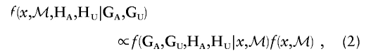
where the summations are over the haplotype pairs consistent with the observed genotypes. Here, ℳ denotes a set of model parameters describing the underlying population dynamics and genetic mechanisms, which may include population SNP haplotype frequencies and aspects of the genealogical history of the disease mutation(s). By Bayes’s Theorem, we can derive the following equation:
 |
where  denotes the prior density of the location of the disease locus and model parameters. Since the observed genotypes are completely determined by the constituent haplotypes, equation (1) can be rewritten as
 |
Neglecting the summations, equation (3) is equivalent to the corresponding expression for the haplotype-based analysis of Morris et al. (2002). Thus, COLDMAP, version 2, is the same as version 1 except for an update step for the haplotype configuration: the haplotypes are treated as latent variables, with new configurations proposed—and accepted or rejected—in the same way as for the other model parameters, ℳ.
Modeling Assumptions
We briefly review the modeling assumptions underpinning COLDMAP below (see Morris et al. [2002] for further details). The ancestral history of the sample of case chromosomes at the disease locus is represented by a bifurcating genealogical tree, tracing the descent of genetic material flanking the disease locus from the founder, at the root, to the sampled chromosomes, at the leaves. The prior distribution for the tree is based on the standard coalescent process (Kingman 1982; Nordborg 2003). However, to account for genetic heterogeneity at the disease locus, the standard model has been generalized to allow branches of the genealogical tree to be removed. Under this shattered coalescent process, each node of the genealogy has equal prior probability of having a parental node in the tree. A realization of this process may include single leaves, corresponding to sporadic case chromosomes, as well as disconnected subtrees, each corresponding to a distinct mutation at the disease locus. Single leaves and subtree founders are assumed to correspond to random chromosomes from the background population and are thus modeled in the same way as controls. Founding SNP haplotypes are transmitted through subtrees of the shattered genealogy, occasionally being altered by marker mutation and trimmed by recombination with random chromosomes from the background population.
Although we could use the same representation to model the shared ancestry of control chromosomes, we assume that a pair of chromosomes carrying a mutant disease allele at the disease locus tend to be more closely related than a random pair of chromosomes from the population. Thus, we adopt a simpler, first-order Markov model for control haplotypes. By neglecting their shared ancestry, we reduce the computational burden while making some allowance for background LD between adjacent SNPs.
MCMC Algorithm
The MCMC algorithm of Metropolis type (Metropolis et al. 1953) performs a random walk in the space of unknowns,  . It is designed so that the proportion of time spent in any region of 𝒮 is approximately the probability that the true values lie in that region, given the data and modeling assumptions. At each iteration, a new value, s′∈𝒮, is proposed (see appendix A) and is accepted in place of the current value, s, with probability
 |
where the numerator and denominator in the probability expression are given by equation (2). If the proposed value is not accepted, the current value is retained.
The Markov chain begins at an arbitrary value of s. Convergence can be assessed using standard diagnostics (Gamerman 1997). Autocorrelation between draws is reduced by recording output, after a burn-in period, at every rth iteration of the algorithm, for some suitably large value of r. The recorded outputs then form an approximate random sample from the joint posterior distribution expressed in equation (3). The marginal posterior distribution of the location of the disease locus is approximated from this joint distribution by ignoring all output parameters other than x.
Output from the algorithm may be used to approximate not only the posterior density for location but also for any of the other unknowns, such as haplotype configuration. Furthermore, within the Bayesian MCMC framework, it is straightforward to incorporate missing SNP genotype information from the sample. Initially, genotypes are arbitrarily assigned to each untyped locus and are updated in the same way as any other unknowns. The COLDMAP Linux executable and accompanying documentation are available, on request, from the corresponding author.
Simulation Study
We consider a 950-kb candidate region, spanned by 20 SNPs at equal 50-kb intervals. The interval includes a single disease locus that is located at random. The joint ancestry of 20,000 haplotypes is generated via a realization of the ancestral recombination graph (ARG) (Hudson 1983; Griffiths and Marjoram 1996, 1997), assuming a recombination rate of 1 cM/Mb, constant both over time and over the interval. For each SNP, the position of a single mutation event in the ARG is selected at random, subject to the constraint that the minor allele frequency is >10%, which approximates the nonascertainment of rare SNPs. Similarly, the position of a single disease-predisposing mutation is selected at random in the ARG, subject to the constraint that the relative frequency of the mutant allele is ∼0.25 (thus, our simulations assume a common disease-predisposing variant). Placing mutations on a realization of the ARG (no data) is not the same as generating a genealogy under the ARG conditional on the haplotype data. The former approach is simpler than the latter, and additional simulations suggest that the differences that arise are negligible for fine mapping (results not shown).
The haplotypes are paired randomly (i.e., assuming Hardy-Weinberg equilibrium) to form 10,000 diplotypes, to which phenotypes are assigned under a range of disease models (table 1), based on the number of mutant alleles (0, 1, or 2) at the disease locus. Finally, 100 cases and 100 controls are sampled and are used for three COLDMAP analyses:
-
1.
Version 1, using the true haplotypes (HAPLOTYPE);
-
2.
Version 1, using haplotypes inferred by SNPHAP from unphased case genotypes and, separately, from unphased control genotypes (INFERRED); and
-
3.
Version 2, using unphased genotypes (GENOTYPE).
Although PHASE, which implements a pseudo-Gibbs sampler, may be superior to SNPHAP, which implements maximum-likelihood inference using an expectation-maximization (EM) algorithm, we used the latter because of the computational resources required by the former for our 1,800 data sets.
Table 1.
Disease Models for the Simulation Study [Note]
|
Disease LocusGenotype RelativeRisk |
Expected No. of Cases |
|||||
| DiseaseModel | Allelic OR | 1 Mutant | 2 Mutants | 0 Mutants | 1 Mutant | 2 Mutants |
| 1 | 25.6 | 1 | 100 | 8 | 5 | 87 |
| 2 | 13.2 | 1 | 50 | 14 | 9 | 77 |
| 3 | 12.4 | 1.5 | 50 | 13 | 13 | 74 |
| 4 | 5.7 | 1 | 20 | 26 | 17 | 57 |
| 5 | 5.6 | 1.5 | 20 | 24 | 24 | 53 |
| 6 | 5.2 | 2 | 20 | 22 | 29 | 49 |
| 7 | 3.3 | 1 | 10 | 36 | 24 | 40 |
| 8 | 3.3 | 1.5 | 10 | 32 | 32 | 36 |
| 9 | 3.2 | 2 | 10 | 29 | 39 | 32 |
| 10 | 3.1 | 5 | 10 | 18 | 62 | 20 |
| 11 | 3.1 | 10 | 10 | 11 | 76 | 13 |
| 12 | 2.5 | 5 | 5 | 20 | 69 | 11 |
| 13 | 2.2 | 2 | 5 | 35 | 46 | 19 |
| 14 | 2.1 | 1.5 | 5 | 39 | 39 | 22 |
| 15 | 2.0 | 1 | 5 | 45 | 30 | 25 |
| 16 | 1.6 | 2 | 2 | 39 | 52 | 9 |
| 17 | 1.4 | 1.5 | 2 | 45 | 45 | 10 |
| 18 | 1.3 | 1 | 2 | 53 | 35 | 12 |
Note.— Allelic OR is the ratio of the odds that a case allele is a mutant to the odds for a control (the latter is 1:3). For each model, the expected numbers of controls with 0, 1, and 2 copies of the mutant allele are 56, 38, and 6, respectively.
Approximations to the posterior distribution of the location of the disease locus are obtained from the output of the MCMC algorithm, starting from the same random parameter configuration for each of the three analyses and assuming the correct recombination rate of 1 cM/Mb. The SNP mutation rate was taken to be 5×10⁻⁵/locus/chromosome/generation. Note that, under our simulation approach, there is no “true” mutation rate; we follow our usual practice of adopting a relatively large value because it helps with mixing of the MCMC algorithm and can allow for some genotyping errors for real data. Furthermore, we have found that location inferences are insensitive to the assumed marker mutation rate over a wide interval (results not shown). Each run of the algorithm consists of a 20,000 iteration burn-in period, followed by a 50,000 iteration sampling period, during which output is recorded at every 50th iteration. The mean run times on a dedicated Pentium III processor were 33 h for each of the haplotype-based version 1 analyses and 45 h for the genotype-based version 2 analysis.
Results
For each of the 18 disease models and 3 data formats, we measured the quality of estimation of the location of the disease locus by the root mean integrated square error (RMISE), averaged over the 100 replicate data sets (fig. 1). For each data set, the RMISE is approximated by the square root of the average squared difference between the 1,000 location outputs from the MCMC algorithm and the true location of the disease locus. As expected, the RMISE tends to be larger for disease loci with small effect, measured by the allelic odds ratio (OR). Furthermore, the HAPLOTYPE analysis generally has the lowest RMISE, and the INFERRED analysis has the largest. On average, over the disease models considered here, the HAPLOTYPE analysis gives an RMISE 6% smaller than does the GENOTYPE analysis (143 kb versus 152 kb [SE 2.6 kb]), whereas the INFERRED analysis gives a 20% larger RMISE (183 kb [SE 3.4 kb]). Note that the performance of the INFERRED analysis is likely to be strongly dependent on marker spacing, and its relative inefficiency may be lessened for more densely spaced SNP markers.
Figure 1.

Approximate RMISE (kb) of the location of the disease locus, averaged over 100 replicate data sets for each of three data formats, against log(allelic OR). The SE of each estimate is ∼11 kb for the HAPLOTYPE and GENOTYPE data formats and 13 kb for INFERRED.
Table 2 presents the mean (over 100 replicates) of the width (kb) and coverage of 50% equal-tailed posterior credibility intervals for the location of the disease locus. As expected, the interval widths tend to increase as the effect of the disease mutant (the allelic OR) diminishes. The intervals for the HAPLOTYPE analysis are always narrower than for the GENOTYPE analysis—on average, about one-third narrower. This reflects the uncertainty in phase assignment, but it is also partly due to the lower achieved coverage of the HAPLOTYPE intervals (on average, 46% versus 52% for GENOTYPE; the former is significantly different from the nominal 50%, but the latter is not). The credibility intervals for the INFERRED analysis are even narrower than for the HAPLOTYPE analyses, but they have greatly reduced coverage, averaging only 19%. This reflects the overconfidence arising from the fact that reconstructed haplotypes tend to exaggerate LD, together with the implicit, but often false, assumption that the reconstructed haplotypes are correct.
Table 2.
Mean Width and Achieved Coverage of 50% Equal-Tailed Posterior Credibility Intervals for the Location of the Disease Locus for Three Data Formats [Note]
|
Mean Width in kb (Achieved Coverage)for Data Format |
||||
| DiseaseModel | Allelic OR | HAPLOTYPE | GENOTYPE | INFERRED |
| 1 | 25.6 | 97 (45%) | 126 (48%) | 71 (30%)a |
| 2 | 13.2 | 106 (49%) | 144 (54%) | 71 (19%)a |
| 3 | 12.4 | 113 (54%) | 165 (68%)a | 78 (38%)a |
| 4 | 5.7 | 126 (48%) | 192 (55%) | 81 (26%)a |
| 5 | 5.6 | 136 (53%) | 187 (57%) | 93 (33%)a |
| 6 | 5.2 | 114 (47%) | 180 (56%) | 79 (16%)a |
| 7 | 3.3 | 110 (44%) | 191 (53%) | 84 (28%)a |
| 8 | 3.3 | 113 (44%) | 188 (50%) | 87 (8%)a |
| 9 | 3.2 | 122 (45%) | 203 (50%) | 89 (14%)a |
| 10 | 3.1 | 105 (48%) | 174 (50%) | 81 (19%)a |
| 11 | 3.1 | 125 (47%) | 183 (52%) | 92 (24%)a |
| 12 | 2.5 | 111 (42%) | 203 (45%) | 101 (11%)a |
| 13 | 2.2 | 120 (44%) | 205 (48%) | 87 (14%)a |
| 14 | 2.1 | 119 (48%) | 202 (52%) | 90 (10%)a |
| 15 | 2.0 | 128 (46%) | 213 (51%) | 94 (13%)a |
| 16 | 1.6 | 119 (38%)a | 198 (44%) | 93 (14%)a |
| 17 | 1.4 | 127 (41%) | 208 (48%) | 96 (17%)a |
| 18 | 1.3 | 120 (40%)a | 226 (46%) | 109 (12%)a |
| Average | … | 117 (46%) | 188 (52%) | 88 (19%) |
Note.— Observed over 100 replicate data sets.
Interval not consistent with nominal coverage probabilities.
Example Application
Hosking et al. (2002) genotyped 1,018 individuals at 32 SNP markers across an 890-kb region flanking the CYP2D6 gene on human chromosome 22q13. By typing four functional polymorphisms in CYP2D6, 41 individuals were found to carry two mutant alleles and, hence, were predicted to have the poor drug metabolizer phenotype. Figure 2 presents the results of a single-locus analysis of the marker SNPs that highlighted a 403-kb region in high LD with this predicted phenotype, which included CYP2D6 (indicated by the vertical dashed lines). Morris et al. (2003) analyzed the unphased genotypes directly by use of version 2 of COLDMAP, identifying a 95% credibility interval for location with width of just 185 kb, including CYP2D6, but with less than half the width of the region of high LD (fig. 2).
Figure 2.

Approximate location of the CYP2D6 locus underlying predicted poor drug metabolizer phenotype within an 890-kb candidate region studied by Hosking et al. (2002). The curves indicate the approximate posterior distributions of the location of CYP2D6 under a version 1 COLDMAP analysis of inferred haplotypes and a version 2 COLDMAP analysis of unphased genotypes. The circles indicate −log10(p-values) from single-locus analyses of marker SNPs. The vertical lines below the X-axis show the 403-kb high-LD region and the 95% credibility intervals for location from the two COLDMAP analyses. The location of CYP2D6 is represented by the vertical dashed lines.
For comparison, we have inferred the SNP haplotypes of predicted poor metabolizer cases, as well as those of controls, by use of SNPHAP. We have then performed a version 1 COLDMAP analysis of the reconstructed haplotypes, treating them as if they were correct. For the version 2 analysis, we have assumed a constant recombination rate of 1 cM/Mb across the region and a marker mutation rate of 2.5×10⁻⁵/locus/generation. The algorithm was run for an initial burn-in period of 10,000 iterations, followed by a 40,000 iteration sampling period during which output is recorded at every 10th iteration. Figure 2 presents the approximate posterior distribution of the location of CYP2D6, obtained from a single run of the algorithm. The 95% credibility interval for the inferred haplotypes analysis does not include the true location of CYP2D6, providing further evidence against the two-stage approach to gene mapping with unphased genotypes.
Discussion
We have shown that an appropriate genotype-based analysis for LD fine mapping in a candidate region can be almost as efficient as an analysis that is based on true haplotypes. In contrast, a two-stage analysis, in which haplotypes are inferred from unphased genotypes using an EM algorithm and are subsequently analyzed as if they were true haplotypes, can be very inefficient. This conclusion is based on markers spaced at 50 kb, and haplotype inferral is likely to be more precise for more densely spaced markers, although we expect the same qualitative differences for any density. Furthermore, our simulations have assumed a constant recombination rate throughout the candidate region, whereas evidence is accumulating for substantial fine-scale variation in recombination rates (see, e.g., Jeffreys et al. 2001). However, Phillips et al. (2003) have shown that chromosomewide patterns of LD are broadly consistent with a constant recombination rate, and we expect our qualitative conclusions to be robust to recombination-rate variation.
We might also expect more sophisticated methods of haplotype reconstruction to improve the efficiency of the two-stage approach, although it is difficult to predict to what extent the efficiency may improve. In particular, we have noted that PHASE may be superior to the EM algorithm, but we used the latter because of the computational requirements of PHASE in our large simulation study. Whatever method of haplotype reconstruction is employed, it seems unlikely that the problems inherent in the two-stage approach—the loss of information and the exaggeration of LD—can be entirely eliminated. The overoptimism of the resulting interval and variance estimates will also remain if the inferred haplotypes are treated as known in the second stage.
Our results are consistent over a broad range of disease models (table 2) (fig. 1). Lu et al. (2003) consider two disease models, one Mendelian and one complex, analyzed using both the BLADE algorithm (Liu et al. 2001) and DHSmap (McPeek and Strahs 1999). For the Mendelian disease example, their results are in accord with our finding that the two-stage approach leads to a loss of efficiency for fine mapping. For their complex disease model, however, they argue for a slight advantage of the two-stage approach, because for complex diseases “…jointly modeling haplotype uncertainty and disease location may only add to the model complexity without having an appropriate gain.” COLDMAP is based on the shattered coalescent model, which incorporates the genealogical structure of the cases while allowing for sporadics and mutation heterogeneity and does seem able to extract an “appropriate gain,” even when the allelic OR is low.
If our conclusions are accepted, then attempts to fine-map disease loci should avoid the two-stage approach and seek appropriate genotype-based statistical analyses. However, until recently, there has been little methodology available for genotype-based fine mapping. We have contributed to filling this methodology gap by extending our COLDMAP algorithm to directly handle genotype data. Although it performs well for small-to-moderate–sized data sets (say, up to ∼200 cases and ∼500 controls, at up to 40 SNPs), computational time and mixing problems mean that its use is not yet feasible for large data sets. We are pursuing several approaches to improving its computational efficiency—for example, by the use of simulated tempering (Liu 2001). Alternatively, we could reduce convergence time by employing a haplotype-reconstruction algorithm only for the controls.
Acknowledgments
The authors thank Louise Hosking and Chun-Fang Xu (GlaxoSmithKline, Stevenage, United Kingdom) for providing the CYP2D6 data set. A.P.M. acknowledges the financial support from the Wellcome Trust.
Appendix A : Details of the MCMC Proposals
To ensure reversibility, each proposal of a new parameter configuration, s′∈𝒮, is one of four types of update, selected according to the probability weights shown in table A1 and described below. Note that SNP alleles are coded “1” and “2.”
Table A1.
Weight Assigned to Changes in the Current Parameter Configuration for the COLDMAP MCMC Algorithm[Note]
| Change | Proposal | Parameter | Weight |
| 1 | Location of disease locus | x | 1 |
| 2 | Model parameter | ℳ | 2nA(6 + m) + m−7 |
| 3 | Haplotype configurations | HA, HU | m(nA + nU) |
| 4 | Missing marker information | HA, HU | u |
Note.— nA = cases; nU = controls; m = marker SNPs; u = untyped SNP alleles.
Change 1: Propose a new location for the disease locus. The proposed location is given by  , where ε denotes a standard uniform random variable and ν denotes a constant that controls the maximum change in the location for each proposal. To ensure reversibility, the proposed location is reflected back into the candidate region if x′ lies outside the candidate region.
Change 2: Propose a new value for a model parameter. Select a model parameter, Mi, at random for the proposed change. Make a small change to the selected parameter, as detailed by Morris et al. (2002), ensuring reversibility.
Change 3: Propose a new haplotype configuration. Select an individual, j, and a SNP, m, at random for the proposed change. If m is located to the left of the current location of the disease locus, then
 |
and
 |
where HPjkl denotes the allele present on haplotype l at SNP k, carried by individual j with disease status P. Conversely, if m is located to the right of the current location of the disease locus, then
 |
and
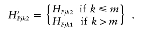 |
Change 4: Propose a new allele for the missing marker information. Choose at random a SNP, m, with missing marker data on haplotype l for individual j with disease phenotype P. The proposed allele is given by H′Pjml=3-HPjml, with HPjml defined as above.
Electronic-Database Information
The URL for data presented herein is as follows:
References
- Clayton D (2000) Linkage disequilibrium mapping of disease susceptibility genes in human populations. Int Stat Rev 68:23–43 [Google Scholar]
- Douglas JA, Boehnke M, Gillanders E, Trent JM, Gruber SB (2001) Experimentally derived haplotypes substantially increase the efficiency of linkage disequilibrium studies. Nat Genet 28:361–364 10.1038/ng582 [DOI] [PubMed] [Google Scholar]
- Gamerman D (1997) Markov chain Monte Carlo: stochastic simulation for Bayesian inference. Chapman and Hall, London [Google Scholar]
- Griffiths RC, Marjoram P (1996) Ancestral inference from samples of DNA sequences with recombination. J Comput Biol 3:479–502 [DOI] [PubMed] [Google Scholar]
- ——— (1997) An ancestral recombination graph. In: Donnelly P, Tavaré S (eds) Progress in population genetics and human evolution. Springer-Verlag, New York, pp 257–270 [Google Scholar]
- Hosking LK, Boyd PR, Xu CF, Nissum M, Cantone K, Purvis IJ, Khakkar R, Barnes MR, Liberwith U, Hagen-Mann K, Ehm MG, Riley JH (2002) Linkage disequilibrium mapping identifies a 390-kb region associated with CYP2D6 poor drug metabolising activity. Pharmacogenomics J 2:165–175 10.1038/sj.tpj.6500096 [DOI] [PubMed] [Google Scholar]
- Hudson RR (1983) Properties of a neutral allele model with intragenic recombination. Theor Popul Biol 23:183–201 [DOI] [PubMed] [Google Scholar]
- Jeffreys AJ, Kauppi L, Neumann R (2001) Intensely punctate meiotic recombination in the class II region of the major histocompatability complex. Nat Genet 29:217–222 10.1038/ng1001-217 [DOI] [PubMed] [Google Scholar]
- Kingman JFC (1982) The coalescent. Stoch Proc Appl 13:235–248 10.1016/0304-4149(82)90011-4 [DOI] [Google Scholar]
- Liu JS (2001) Monte Carlo strategies in scientific computing. Springer-Verlag, New York [Google Scholar]
- Liu JS, Sabatti C, Teng J, Keats BJB, Risch N (2001) Bayesian analysis of haplotypes for linkage disequilibrium mapping. Genome Res 11:1716–1724 10.1101/gr.194801 [DOI] [PMC free article] [PubMed] [Google Scholar]
- Lu X, Niu T, Liu JS (2003) Haplotype information and linkage disequilibrium mapping for single nucleotide polymorphisms. Genome Res 13:2112–2117 10.1101/gr.586803 [DOI] [PMC free article] [PubMed] [Google Scholar]
- McPeek MS, Strahs A (1999) Assessment of linkage disequilibrium by the decay of haplotype sharing, with application to fine-scale genetic mapping. Am J Hum Genet 65:858–875 [DOI] [PMC free article] [PubMed] [Google Scholar]
- Metropolis N, Rosenbluth AW, Rosenbluth MN, Teller AH, Teller E (1953) Equation of state calculations by fast computing machines. J Chem Phys 21:1087–1092 [Google Scholar]
- Morris AP, Whittaker JC, Balding DJ (2002) Fine-scale mapping of disease loci via shattered coalescent modeling of genealogies. Am J Hum Genet 70:686–707 [DOI] [PMC free article] [PubMed] [Google Scholar]
- Morris AP, Whittaker JC, Xu CF, Hosking L, Balding DJ (2003) Multipoint linkage disequilibrium mapping narrows location interval and identifies mutation heterogeneity. Proc Natl Acad Sci USA 100:13442–13446 10.1073/pnas.2235031100 [DOI] [PMC free article] [PubMed] [Google Scholar]
- Nordborg M (2003) Coalescent theory. In: Balding DJ, Bishop M, Cannings C (eds) Handbook of statistical genetics, 2nd ed. John Wiley & Sons, Chichester, UK, pp 602–635 [Google Scholar]
- Phillips MS, Lawrence R, Sachidanandam R, Morris AP, Balding DJ, Donaldson MA, Studebaker JF, et al (2003) Chromosome-wide distribution of haplotype blocks and the role of recombination hot spots. Nat Genet 33:382–387 10.1038/ng1100 [DOI] [PubMed] [Google Scholar]
- Schaid DJ (2002) Relative efficiency of unambiguous vs. directly measured haplotype frequencies. Genet Epidemiol 23:426–443 10.1002/gepi.10184 [DOI] [PubMed] [Google Scholar]
- Stephens M, Donnelly P (2003) A comparison of Bayesian methods for haplotype reconstruction from population genetic data. Am J Hum Genet 73:1162–1169 [DOI] [PMC free article] [PubMed] [Google Scholar]
- Stephens M, Smith NJ, Donnelly P (2001) A new statistical method for haplotype reconstruction from population data. Am J Hum Genet 68:978–989 [DOI] [PMC free article] [PubMed] [Google Scholar]