Design and Analysis of Admixture Mapping Studies

Abstract

Admixture between populations originating on different continents can be exploited to detect disease susceptibility loci at which risk alleles are distributed differentially between these populations. We first examine the statistical power and mapping resolution of this approach in the limiting situation in which gamete admixture and locus ancestry are measured without uncertainty. We show that, for a rare disease, the most efficient design is to study affected individuals only. In a typical African American population (two-way admixture proportions 0.8/0.2, ancestry crossover rate 2 per 100 cM), a study of 800 affected individuals has 90% power to detect at P values <10⁻⁵ a locus that generates a risk ratio of 2 between populations, with an expected mapping resolution (size of 95% confidence region for the position of the locus) of 4 cM. In practice, to infer locus ancestry from marker data requires Bayesian computationally intensive methods, as implemented in the program ADMIXMAP. Affected-only study designs require strong prior information on the frequencies of each allele given locus ancestry. We show how data from unadmixed and admixed populations can be combined to estimate these ancestry-specific allele frequencies within the admixed population under study, allowing for variation between allele frequencies in unadmixed and admixed populations. Using simulated data based on the genetic structure of the African American population, we show that 60% of information can be extracted in a test for linkage using markers with an ancestry information content of 36% at 3-cM spacing. As in classic linkage studies, the most efficient strategy is to use markers at a moderate density for an initial genome search and then to saturate regions of putative linkage with additional markers, to extract nearly all information about locus ancestry.

Background

Admixture between ethnic groups that differ in disease risk for genetic reasons provides an experiment of nature that can, in principle, be exploited to localize genes in the same manner as an experimental cross. Although advanced statistical methods are required to apply this approach, in practice, the underlying principle on which it relies to detect linkage is simple. Suppose, for instance, that risk alleles at a locus are differentially distributed between populations so as to generate a twofold higher risk of osteoporotic fractures in Europeans compared with West Africans. If we classify individuals of mixed European/West African descent according to whether they have 0, 1, or 2 gene copies of European ancestry at this locus, disease risk will be twofold higher in those with 2 copies than in those with 0 gene copies of European ancestry. We do not have to compare disease risk between these three groups directly (which would require a cohort design). Instead we can study cases only, comparing at each locus on each gamete the observed and expected proportions of gene copies that have European ancestry.

Although the theory of this approach was outlined by McKeigue (1998), its practical application has awaited the development of statistical methods and panels of markers that are informative for ancestry. To generalize the methods used for linkage analysis of an experimental cross between inbred strains to recently admixed human populations, three main problems must be overcome:

• 1. Confounding by population stratification. In an experimental cross, all individuals have the same history of admixture. In admixed human populations, the history of admixture is not known, and proportionate admixture varies between individuals. This gives rise to associations of the disease with ancestry at unlinked loci. This problem is overcome by conditioning on the admixture proportions of each individual’s parents (McKeigue 1998). To condition on parental admixture, we can either adjust for parental admixture in a generalized linear model (Hoggart et al. 2003) or compare observed locus ancestry with expected locus ancestry (given parental admixture) within each individual.
• 2. Human ethnic groups are not inbred strains. Experimental crosses are usually undertaken using inbred strains, through use of marker loci at which different alleles have been fixed in each strain. For human populations defined by ancestral continent of origin, we can preselect markers that show extreme allele frequency differentials between these continental group populations. However, even these markers will not be perfectly informative for ancestry. This problem can be overcome by a multipoint analysis that combines information from all markers on the chromosome to extract information about ancestry at each locus (Falush et al. 2003; Hoggart et al. 2003).
• 3. Allele frequencies in the ancestral populations are unknown. In an experimental cross, allele frequencies in the ancestral strains are known. For an admixed human population, estimates of the ancestry-specific allele frequencies—the probabilities of each allele, given the ancestry of the gamete at the locus under study—are subject to uncertainty. This is because the ancestral subpopulations that contributed to the admixed population cannot usually be defined precisely and, for some of these subpopulations, no unadmixed descendants are available for study. This problem is overcome by combining data from unadmixed and admixed populations to estimate the ancestry-specific allele frequencies, as described in this article.

Similar problems arise in the analysis of experimental crosses between outbred lines in which grandparents have not been typed (Sillanpaa and Arjas 1999) and in fine mapping of quantitative trait loci through use of heterogeneous stocks of mice (Mott et al. 2000).

Study Designs and Statistical Power of Admixture Mapping

In this section, we examine the statistical power of admixture mapping in the limiting situation in which locus ancestry and gamete admixture proportions are measured without uncertainty. We show later that these conditions can be nearly met if a genomewide panel of ancestry-informative markers is typed and regions of putative linkage are then saturated with additional markers to extract a high proportion of information about locus ancestry.

Comparison of Study Designs

We begin by comparing two alternative study designs and statistical tests for linkage with a binary trait/disease: (1) an affected-only test comparing the observed and expected proportions of gametes that have ancestry from the high-risk subpopulation and (2) a case-control test based on testing for association of disease with locus ancestry from the high-risk population in a logistic regression model. In deriving the tests below, we assume that the test is evaluated at the disease locus. The arguments below apply to both monogenic and oligogenic disease models. Although we consider only tests of the effect of a single locus, the arguments can easily be extended to construct tests for joint effects of two or more loci, as proposed for studies of allelic association (Devlin et al. 2003; Kilpikari and Sillanpaa 2003).

• 1.
  Affected-only test. The unit of observation is a single gamete. The parameter of interest is the ancestry risk ratio r, the risk ratio for disease in those with 2 versus 0 gene copies who have ancestry from the high-risk subpopulation at the locus under study, based on a multiplicative model for risk as a function of number of copies of the high-risk allele. The probability z_r of observing locus ancestry from the high-risk population, given that the gamete is from an affected individual and has admixture proportion θ from the high-risk subpopulation, is (McKeigue 1998)

  

  The likelihood of the observed locus ancestry state A (an indicator variable scored as 0 for ancestry from the low-risk subpopulation and as 1 for ancestry from the high-risk subpopulation) is therefore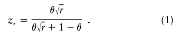

  
• 2.
  Case-control test. The unit of observation is a single individual, and the parameter of interest is the log odds ratio β for disease in those with 2 versus 0 gene copies from the high-risk subpopulation at the locus under study. The test is equivalent to testing the hypothesis β=0 in a logistic regression model. This test can also be applied to a cross-sectional or cohort study of a binary trait. If we ignore confounding by gamete admixture, the model can be specified as

  

  giving the likelihood of the observed individual’s disease status as

  

  where x is the proportion of gene copies that have ancestry from the high-risk subpopulation (0, 1/2, or 1); θ is the mean admixture proportion of the individual’s two gametes; β is the log odds ratio for disease in individuals with 2 versus 0 gene copies who have ancestry from the high-risk subpopulation; p is the prevalence of disease in the study sample (fixed to be 1/2 in a case-control study with equal numbers of cases and controls); Π is the probability that the individual is affected, given p, x, θ, and β; and d is an indicator variable for disease status (0 = control; 1 = case). Specifying the model with the explanatory variable x centered about its expectation θ eliminates covariance between β (the parameter under test) and the intercept.

Tests for linkage can be derived from the likelihood functions given by equations (2) and (3). For a quantitative trait, similar tests can be constructed for the effect of locus ancestry in a linear regression model. The asymptotic approximation of the log likelihood to a quadratic function is improved if the parameter under test is transformed (where necessary) to lie on the real line. Thus, for the affected-only test, the log likelihood is evaluated as a function of logr rather than r.

The statistical power to detect an effect of given size in any given study design can be calculated from the expected information, defined as minus the expectation of the second derivative of the log likelihood with respect to the parameter under test. Table 1 lists, for different study designs, the parameter under test, the log likelihood of a single observation at the trait locus, and the expected information (at the null value of the parameter) contributed by an individual with two gametes that have proportionate admixture θ from the high-risk subpopulation. For comparison of the study designs, the expected information for the affected-only study was calculated with respect to the log-odds ratio β rather than logr. For a rare disease, β≈logr.

Table 1.

Expected Information from Various Study Designs for Admixture Mapping^[Note]

Study Design	Parameter under Test	Log Likelihood of One Observation	Expected Information from Two Gametes with AdmixtureProportions θ
Affected-only	logr, where r is ancestry risk ratio	(for one gamete)
Affected-only with disease prevalence ψ	β, log of ancestry odds ratio	As above, with r expressed in terms of ψ, β
Case-control with case/control ratio p/(1-p)	β, log of ancestry odds ratio
Cross-sectional study of quantitative trait with mean α, residual variance σ2	β, ancestry effect

Note.— θ = proportionate admixture of the gamete from the high-risk ancestry; d = indicator variable for case-control status; x = proportion of gene copies that have ancestry from the high-risk ancestry.

Table 1 shows that the expected information at β=0 contributed by a single individual in a case-control design is p(1-p)/(1-ψ)² times the expected information from an affected-only study. For a rare disease ((1-ψ)²≈1), a case-control design with cases and controls (p=1/2) has one-quarter of the expected information of an affected-only test with n cases. Only if ψ=0.5 is a case-control design as efficient as an affected-only design. If ψ>0.5 (prevalence >50%), it is more efficient to study controls only. These results apply to any test based on the likelihood function.

Statistical Power Calculations

To detect a locus that generates an effect size of λ (where λ can be either the log odds ratio β or the log risk ratio logr) with type I error probability a and type II error probability b, the required number of observations n is given by

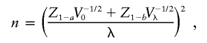where V₀ and V_λ denote the expected information contributed by a single observation under the null and the alternative hypotheses, respectively. In an affected-only design, the expected information contributed by a single gamete with proportionate admixture θ from the high-risk subpopulation is

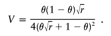For fixed r, V is maximized at θ=(1+r^1/4)^-1. Thus, the most informative gametes are those with slightly less than 50% admixture from the high-risk subpopulation. For modest effect size, V_λ≈V₀ and

Thus, from equation (4), the required information nV₀ for 90% power (Z_1-b=1.28) to detect an effect of size λ=1 at a one-sided P value of <10⁻⁵ (Z_1-a=4.27) is approximated by . The sample size required for 90% power to detect an effect of unit size at a P value of <10⁻⁵ is easily calculated by dividing the required information (30.8) by the expected information from a single observation, given in the last column of table 1. The required sample size for any other effect size is calculated by dividing these numbers by the square of the effect size. Thus, in African American populations, in which the average proportion θ of West African admixture is ∼0.8 (Parra et al. 1998), an affected-only design would require 800 individuals for 90% power to detect, at a P value <10⁻⁵, a locus contributing an ancestry risk ratio r=2 (logr=0.69).

Statistical Modeling

The theoretical results outlined above are based on the assumption that gamete admixture and locus ancestry can be inferred without uncertainty. In reality, marker data will yield only imperfect information about gamete admixture and locus ancestry. We have previously described how the program ADMIXMAP, which models admixture, can be used to control for confounding by population stratification in genetic association studies (Hoggart et al. 2003; Genetic Epidemiology Group Web site). We now describe the application of this program to admixture mapping.

Modeling Admixture

The basic model fitted by ADMIXMAP has been described in detail previously by Hoggart et al. (2003). (Computational methods are described in appendix A.) A similar model is fitted by the program STRUCTURE (Falush et al. 2003). The population under study is modeled as formed by admixture between k ancestral subpopulations. We define “gamete admixture” as the proportion of the parent’s genome that has ancestry from each subpopulation; this is not quite the same as the proportion of the gamete’s genome that has ancestry from each subpopulation. The distribution of gamete admixture in the admixed population is modeled by a Dirichlet distribution with parameter vector α=(α₁,…,α_k). Two alternative models for gamete assortment can be specified in ADMIXMAP: a random-mating model, in which the two parental gametes are drawn independently from this Dirichlet distribution; or an assortative-mating model, in which admixture proportions in the two parental gametes are the same. These alternatives represent extremes; in principle, the model could be extended to estimate the degree to which mating is assortative for individual admixture.

The stochastic variation of ancestry across loci on each gamete is modeled by k independent Poisson arrival processes. Since the relative intensities of these arrival processes are specified by the admixture proportions of the gamete θ, this requires only one extra parameter: the sum of the intensities of the arrival processes, denoted by τ. Although the stochastic variation of ancestry does not exactly follow the model of independent Poisson arrival processes, even under the assumption of no interference (McKeigue 1998), this modeling assumption simplifies the problem. Where admixture has occurred in a single pulse, the expected value of τ is the number of generations that have elapsed since unadmixed ancestors (Falush et al. 2003). The parameter τ determines the resolution of admixture mapping studies and the density of markers required to extract information about ancestry at each locus. With higher values of τ, the mapping resolution will be sharper, but the density of markers required to extract a given proportion of information will also be higher. For a gamete that has admixture proportion θ from a given subpopulation, the ancestry crossover rate ρ (the density of transitions between ancestry from this subpopulation and ancestry from one of the other subpopulations) is given by ρ=2θ(1-θ)τ.

The model assumes no allelic association, conditional on locus ancestry, between loci. Where two or more markers are so close together that this assumption cannot be relied on, these markers are grouped as a single “compound locus.” Ancestry is assumed to be the same at all marker positions within a compound locus on any given gamete, because possible recombination since admixture can be ignored over this short distance. At compound loci, haplotypes and haplotype frequencies are modeled instead of alleles and allele frequencies. Given ancestry at a locus, the likelihood of the observed alleles or unobserved haplotypes is multinomial, with probabilities specified by the ancestry-specific allele (or haplotype) frequencies. The program samples the posterior distribution of the haplotypes and the ancestry-specific allele (or haplotype) frequencies at each locus.

Modeling Dependence of a Trait on Gamete Admixture

For case-control or cross-sectional designs, a generalized linear model is specified for the dependence of the trait on the mean admixture proportions of both gametes, together with any other explanatory variables specified by the user. For a quantitative trait, this is a linear regression model; for a binary trait, this is a logistic regression model. Modeling the dependence of the trait on individual admixture allows the program to use the trait value as well as the genotype data to infer gamete admixture proportions. Even when the test for linkage is evaluated on affected individuals only, including a control group and fitting a logistic regression model will help the model to infer gamete admixture and allele frequencies.

Modeling Allele Frequencies

The probabilities of observing each possible allele or haplotype at a locus, given the ancestry of the gamete at that locus, are specified by the ancestry-specific allele (or haplotype) frequencies in the admixed population. ADMIXMAP allows the ancestry-specific allele frequencies to be specified in one of three ways:

• 1. as constants specified by the user, with a score test for misspecification, as described by McKeigue et al. (2000);
• 2. as random variables with a Dirichlet prior distribution specified by the user (a reference prior [Jeffreys 1961], with all elements of the Dirichlet parameter vector equal to 0.5, can be specified where no allele frequency data are available); and
• 3. as random variables with a “dispersion” model that allows the ancestry-specific allele frequencies in the admixed population to vary from the corresponding frequencies in unadmixed modern descendants.

For most populations formed by recent admixture between continental groups, some information about ancestry-specific allele frequencies is available from sampling modern unadmixed descendants of the continental groups that contributed to the admixed population. We may be prepared to assume that the allele frequencies in these unadmixed descendants are the same as the corresponding ancestry-specific allele frequencies in the admixed population; we denote this as the “no dispersion” assumption. Where allele frequencies have been estimated from relatively small samples of unadmixed individuals, it is necessary to allow for sampling error in the estimates. This is straightforward within a Bayesian framework, in which the posterior distribution from the last study becomes the prior for the next study. Thus, we can specify a Dirichlet prior distribution for the ancestry-specific allele frequencies as the posterior distribution that is obtained by combining a reference prior, Di(0.5,…,0.5), with the likelihood of the data from the unadmixed population. The parameters of this distribution are obtained simply by adding 0.5 to the observed counts of each allele in the unadmixed population sample. We can test the assumption of no dispersion by constructing a model diagnostic based on the posterior predictive check probability, described in appendix B. For each subpopulation, this test compares the likelihood of the observed and replicate allele counts in the admixed population given the ancestry specific allele frequencies. This test is computed at each locus and (by summing the log likelihoods over all loci) as a summary test for each subpopulation.

Where there is evidence that the no-dispersion assumption is violated, we can fit a dispersion model. In comparison with a model that assumes no dispersion, this gives less weight to the allele frequency data from modern unadmixed descendants (the “historic” allele frequencies) when estimating ancestry-specific allele frequencies within the admixed population under study. This is achieved by specifying a hierarchical model for allele frequencies similar to that described by Lockwood et al. (2001). For each continental group, the ancestry-specific allele frequencies in the admixed population and the corresponding “historic” frequencies in the unadmixed population are drawn independently from a Dirichlet distribution, Di(μ). For a locus with a alleles, μ=(μ₁,…,μ_a) and . We reparameterize the Dirichlet distribution such that . The allele frequencies at each locus are distributed as

where i indexes loci and j indexes either a subpopulation within the admixed population (j=1) or the corresponding unadmixed continental group (j=2). The dispersion parameter η controls the variance of the Dirichlet distribution and is specified to be the same for all loci in each continental group. It is related to Wright’s F_st (Wright 1951), by F_st=(1+η)^-1 (Lockwood et al. 2001). In our application, η indexes dispersion between “historic” allele frequencies in modern unadmixed descendants and the corresponding ancestry-specific allele frequencies within the admixed population. Larger values of η imply less dispersion of allele frequencies.

Simulations show that, for the dispersion parameter η to be estimated reliably from data on an admixed population sample with a vague prior distribution, either the marker panel must contain sequences of closely linked markers, so that locus ancestry can be inferred accurately, or admixture proportions must vary widely between the sampled individuals, so that ancestry-specific allele frequencies can be inferred from the dependence of observed allele frequencies on individual admixture proportions. In studies reported so far, we have used only the Penn State marker panel (Shriver et al. 2003), which has only a few short sequences of linked markers. In this situation, it is necessary to assign an informative prior for the dispersion parameter η, based on estimates of the variance of allele frequencies between subpopulations within each continental group. For instance, F_st between subpopulations within West Africa has been estimated as ∼0.02 (Cavalli-Sforza et al. 1994). If dispersion of allele frequencies between modern West Africans and the corresponding ancestry-specific allele frequencies in the African American population is similar to the dispersion between West African subpopulations, this suggests that the prior for η should have its mode at ∼50. Similarly, F_st between subpopulations within Europe has been estimated as ∼0.002, suggesting that the prior for η should have its mode at ∼500. Since the dispersion parameter η will depend on how the markers were selected and what mix of subpopulations within the continental group was sampled to estimate allele frequencies, the prior for η should reflect this uncertainty.

In accordance with the principles of Bayesian inference, we can use the posterior distribution of ancestry-specific allele frequencies generated by ADMIXMAP to specify a prior distribution for these allele frequencies in subsequent studies of new samples from the same admixed population. From this stage onward, we need not specify a dispersion model, as long as we can assume that ancestry-specific allele frequencies do not vary between different samples from the same admixed population. To simplify the computation, the posterior distribution of allele frequencies generated by ADMIXMAP is approximated by a Dirichlet distribution, which can be used to specify a prior for subsequent studies. The parameters of this distribution are calculated by equating the means and the determinant of the covariance matrix of the Dirichlet distribution with the posterior means and the determinant of the posterior covariance matrix of the allele frequencies generated by ADMIXMAP.

Application to Admixture Mapping

Tests for linkage

The tests for linkage provided in ADMIXMAP are score tests based on the missing-data likelihood. With this approach, it is straightforward to test any null hypothesis of the form λ=λ₀, where λ₀ is the value specified in the Bayesian model. The basic algorithm has been described elsewhere (McKeigue et al. 2000; Hoggart et al. 2003). For each realization of the complete data, we calculate the realized score (gradient of the log likelihood at λ₀) and the realized information (minus the second derivative of the log likelihood at λ₀). For an affected-only study testing the null hypothesis logr=0, the realized score and information for a single gamete at any given locus can be derived from expression (2) as (A-θ)/2 and θ(1-θ)/4, respectively. The score U is evaluated as the posterior expectation of the realized score, and the observed information V is calculated by subtracting the missing information (posterior variance of the realized score) from the complete information (posterior expectation of the realized information). Under the null hypothesis, U^tV^-1U has a χ² distribution.

In comparison with a fully Bayesian approach, this score test algorithm has several advantages: (1) it is computationally efficient, because multiple hypotheses can be tested in a single run of the Markov chain Monte Carlo sampler; (2) it requires only a null model to be fitted, avoiding difficulties (such as ascertainment bias) that may arise away from the null; and (3) the ratio of observed to complete information is a useful estimate of the efficiency of the study design relative to an ideal experiment in which latent variables are measured directly. In large samples, score tests are asymptotically equivalent to likelihood ratio tests. Furthermore, asymptotically, the log likelihood is approximated by a quadratic (see eq. [5]).

An alternative approach to testing for linkage of a particular locus in an affected-only design would be to compute a likelihood ratio that compares the likelihood under the null hypothesis, H₀, that there is no disease locus linked to the locus under study, with the alternative hypothesis, H₁, that the locus under study contributes a population risk ratio of r.

Information content mapping

An information content map measures the adequacy of a marker set to detect linkage in comparison with an infinitely dense marker map that allows locus ancestry and gamete admixture to be inferred without uncertainty. This allows us to determine where additional markers should be added to the map. We can construct this information content map through use of the ratio of observed to complete information in the affected-only score tests at each locus. For this purpose, the tests should be evaluated on an unselected sample of individuals for whom we can assume that the null hypothesis is true. The information content of the map has to be evaluated separately for each admixed population under study, because it depends on the history of admixture as well as on the ancestry-specific allele frequencies. As in classic linkage studies, there is a trade-off between the marker density required to extract a given proportion of information and the information content of the individual markers.

There are several possible ways to calculate marker information content for ancestry. In this article, the quoted values of marker information content for ancestry are based on the expected proportion f by which the prior variance of locus ancestry on a single gamete is reduced by typing the locus (McKeigue 1998; Molokhia et al. 2003). This measure is useful for our purposes, because it is equivalent to the efficiency that the affected-only score test would have if no information from linked marker loci were available. An alternative measure, I_n, has been suggested by Rosenberg et al. (2003). Although absolute values of f and I_n differ, both measures rank markers similarly with respect to information content.

Exclusion mapping

An exclusion map shows, at each position on the genome, the effect size r that can be excluded at a given LOD score threshold. This can be used to exclude regions from typing additional markers, because the data already obtained are sufficient to exclude an effect of the size that the study was designed to detect. To construct an exclusion map, we require the log likelihood as a function of the effect size at each locus. As noted above, a quadratic function that approximates the log likelihood —say, ℒ—can be obtained from the score U and information V calculated in the score test. For an affected-only test, the log likelihood is evaluated as a function of ; if we arbitrarily set ℒ=0, this function is

To compute exclusion thresholds based on the traditional criterion of a LOD score of −2, we can substitute and solve this quadratic equation to calculate two values of r at which the likelihood is 100 times lower than the likelihood at r=1. Comparison with the true log-likelihood function (calculated in the limiting situation in which gamete admixture and locus ancestry are measured without uncertainty) shows that this approximation is fairly accurate, except at values of r that are far from the null, which are not relevant to exclusion mapping.

Mapping Resolution

The expected size of the confidence region for the position of a disease locus detected by admixture mapping with an affected-only design can be calculated by adapting the approach used by Kruglyak and Lander (1995b) to generate the probability distribution of the size of the confidence region in linkage studies of affected relative pairs. We assume that gamete admixture and locus ancestry are measured without uncertainty, as in the limiting situation in which an infinitely dense marker map has been typed. For a single gamete from an affected individual, the probability z_r of ancestry from the high-risk subpopulation at the disease locus is given by equation (1). It follows that the likelihood ratio contrasting the hypothesis that a disease locus with effect size r is at a given map position with the hypothesis that this position is unlinked to the disease is the ratio of two Bernoulli likelihoods with parameters z_r and θ, respectively.

Kruglyak and Lander (1995b) use the theory of random walks to derive an approximation for the distribution of the size of a confidence region C_γ that has probability γ of containing the disease locus. In the region of the disease locus, the LOD score behaves approximately as a random walk conditioned to pass through its expected value at the disease locus. In an affected-only mapping study, this walk has constant step size,

with upward and downward step probabilities of π and 1-π respectively, where

The confidence region C_γ is defined as the smallest interval containing all points at which the LOD score exceeds a threshold level Z^*-T_γ, where Z^* is the maximum LOD score. T_γ is given by .

To calculate the distribution of the size of the confidence region, we require the distribution of the number of transitions S required for the LOD score to drop permanently below Z^*-T_γ. In an affected relative-pair study, these transitions are between sharing 0 and 1 gene copies on pairs of gametes inherited from a common ancestor. In an admixture mapping study, the transitions are between states of ancestry from low-risk and high-risk subpopulations on single gametes. These transitions are modeled as a Poisson arrival process with intensity parameter ν=[ρ₊(1-z_r)+ρ_-z_r]n per morgan in the region of the disease susceptibility locus, where n is the number of affected gametes and ρ₊ and ρ_- are the densities of transitions to higher and lower LOD scores, respectively. Thus, for a gamete with proportionate admixture θ from the high-risk subpopulation, the densities of these transitions are given by ρ₊=θτ and ρ_-=(1-θ)τ, where τ is the sum-of-intensities parameter defined above. The average density of ancestry crossovers over all n gametes in the region of the disease locus is ν=[θτ(1-z_r)+(1-θ)τz_r]n per morgan. The distance between successive arrivals follows an exponential distribution with mean 1/ν. It follows that the distance for the arrival of S transitions has a gamma distribution with shape parameter S and scale parameter ν. Samples from this distribution can be generated by simulation, allowing us to compute the distribution of the size of the confidence region C_γ.

Data Sources

Three African American population samples and one Hispanic American population sample were typed for diallelic markers selected from a panel of 38 markers informative for West African, European, and Native American ancestry. The African American samples consisted of a cross-sectional study of 202 individuals in Philadelphia, typed at 26 loci; a cross-sectional study of 232 individuals in Washington, DC, typed at 34 loci (see Shriver et al. [2003] for details of this collection); and 393 individuals resident in the Washington, DC region who were included in a case-control study of prostate cancer, typed at 27 loci (see Kittles et al. [2001] and [2002] for details of this collection). The Hispanic American sample was a cross-sectional sample of residents of San Luis Valley, Colorado, enriched with cases of diabetes ascertained from clinics, typed at 21 marker loci, as described by Hoggart et al. (2003).

Samples of unadmixed West Africans, Europeans, and Native Americans were typed for the same panel of 38 ancestry-informative markers. The West African sample consisted of 369 individuals typed at all 38 loci, the European sample consisted of 229 individuals typed at 35 loci, and the Native American sample consisted of 182 individuals typed at 35 loci. For further details of these data sets, see Shriver et al. (2003).

Results

Estimation of Ancestry Crossover Rate and Mapping Resolution

Table 2 shows estimates of the sum-of-intensities parameter τ based on the three African American samples and the one Hispanic American sample. The 95% credible intervals are wide, since the marker panels used in these studies included only a few sequences of linked markers. Combining these studies, we estimate τ in African Americans to be ∼6 per 100 cM. Falush et al. (2003) estimated τ in a sample of African Americans from Maywood, Illinois to have a posterior mean of 9.8 and a 90% credible region of 7–13.

Table 2.

Posterior Summaries for the Sum-of-Intensities Parameter in Four Admixed Populations

			Sum-of-Intensities Parameter
Population	No. of Individuals	No. of Markers	Median	95% CredibleInterval
African American:
Prostate cancer	393	64	5.7	4.3–7.2
Philadelphia	202	26	6.1	3.3–10.6
Washington, DC	232	33	7.1	4.6–10.8
Hispanic American:
San Luis Valley	446	21	8.1	5.1–12.4

A sum of intensities of 6 implies that, for admixture proportions 0.8/0.2, the ancestry crossover rate is ∼2 per 100 cM (2×0.80×0.20×6). From this, we calculated the expected resolution of admixture mapping studies in African American populations in the limiting situation in which locus ancestry and gamete admixture are measured without uncertainty. Figure 1 shows the median and upper 95th percentile of the distribution of the size of the confidence region, plotted against the ancestry risk ratio r for a sample size of 800 individuals with admixture proportion 0.8 from the high-risk population and τ=6. For r=2, the expected size of the confidence region is 4 cM. Since the scale parameter ν has a linear relationship with the sample size n, the expectation of the size of the confidence region is proportional to 1/n. Thus for an expected mapping resolution of 1 cM, ∼3,200 individuals would be required for a locus with ancestry risk ratio r=2, and ∼9,000 individuals for r=1.5.

Figure 1.

Median and upper 95th percentile of the size of the 95% confidence region for the position of a disease locus plotted against the risk ratio for a fixed sample size of 800 individuals with admixture proportion 0.8 from the high-risk population and τ=6.

Testing for Linkage, Information Content Mapping, and Exclusion Mapping

To demonstrate the application of ADMIXMAP to admixture mapping with a dense marker map, we simulated an affected-only study based on the genetic structure of the African American population specified as two-way admixture with admixture proportion θ=0.8 from the high-risk population and sum-of-intensities τ=6 per morgan. For each individual, marker genotypes were generated on two chromosomes 100 cM long with markers spaced every 1 cM, one containing a disease locus that generates an ancestry risk ratio of 2 located halfway along the chromosome, and the other with no disease locus. These markers were diallelic, with the frequency of allele 1 specified as 0.8 in the high-risk subpopulation and as 0.2 in the low-risk subpopulation (equivalent to an information content for ancestry of f=0.36 [McKeigue 1998] or I_n=0.28 [Rosenberg et al. 2003]). Both data sets also included 200 unlinked diallelic markers that were fully informative for ancestry to represent the information on gamete admixture that would be available from typing several hundred other ancestry-informative markers across the genome.

Three analyses of this simulated study with ADMIXMAP were undertaken: (1) one using genotype data at all marker loci; (2) one with genotypes at every second and third linked marker locus set to “missing” on the two chromosomes, to simulate a study with markers evenly spaced at 3 cM; and (3) one using 33 randomly chosen markers on each of the two chromosomes, to simulate a study with markers unevenly spaced at an average spacing of 3 cM. Including the loci with missing genotypes ensures that the program will calculate the proportion of information extracted at these positions, so that we can evaluate the extent to which information extracted falls off between marker loci. Figure 2 shows the P values calculated in the score tests across the chromosome containing the disease locus from all three analyses. In each analysis, linkage is detected over a broad region. Figure 3 shows the proportion of information extracted on the chromosome without the disease locus. With a marker spacing of 1 cM, the proportion of information extracted is >80% for the middle 90% of the chromosome. With markers evenly spaced at 3 cM, the proportion of information extracted is ∼60% for the middle 90% of the chromosome, and the information falls only slightly between marker loci. With an average 3-cM spacing but randomly spaced markers, the information falls to ∼50% between some marker loci. Figures 4 and 5 display the estimated thresholds beyond which an ancestry risk ratio r at the locus can be excluded at a LOD score of −2, for the chromosome containing the disease locus and the chromosome without a disease locus, respectively. Even with markers at 3-cM spacing, an ancestry risk ratio r⩾2 is excluded at a LOD score of −2 over the entire chromosome with no disease locus. On the chromosome containing the disease locus, the regions over which an ancestry risk ratio >2 can be excluded are larger with markers spaced every 1 cM than with markers spaced every 3 cM.

Figure 2.

Plots of P values for simulated data from a chromosome of length 100 cM with disease locus responsible for a risk ratio of 2 at 50 cM. Solid line, markers spaced every 1 cM; dotted line, markers spaced every 3 cM; dashed line, markers randomly spaced with an average spacing of 3 cM.

Figure 3.

Information content map for simulated data from a chromosome of length 100 cM without a disease locus. Solid line, markers spaced every 1 cM; dotted line, markers spaced every 3 cM; dashed line, markers randomly spaced with an average spacing of 3 cM.

Figure 4.

Exclusion map for simulated data from a chromosome of length 100 cM with disease locus responsible for a risk ratio of 2 at 50 cM. Solid line, markers spaced every 1 cM; dotted line, markers spaced every 3 cM; dashed line, markers randomly spaced with an average spacing of 3 cM.

Figure 5.

Exclusion map for simulated data from a chromosome of length 100 cM without a disease locus. Solid line, markers spaced every 1 cM; dotted line, markers spaced every 3 cM; dashed line, markers randomly spaced with an average spacing of 3 cM.

Estimation of Ancestry-Specific Allele/Haplotype Frequencies

To test the ability to learn about ancestry-specific allele frequencies from successive samples from the same admixed population under study, we used the three African American data sets described above. In total, the three data sets included 37 ancestry-informative markers, of which 23 were common to all three data sets; details of the markers are given by Shriver et al. (2003). The model was specified with three subpopulations: West African, European, and Native American. If we assume that ancestry-specific allele frequencies in the African American population do not vary with area of residence, successive updates of the ancestry-specific allele frequencies should yield successively closer fits of the estimated allele frequencies to the true values. To test this prediction, we computed two sets of allele frequency estimates: (1) estimates obtained as the mean frequencies in samples from unadmixed West African populations and (2) estimates obtained as the mean of the posterior distribution obtained by fitting a dispersion model with “historic” allele frequencies given by samples from the unadmixed West African populations and from the Washington, DC and Philadelphia data sets as the admixed populations under study. Since the number of markers in these studies was too small for reliable inference on the dispersion parameters, informative priors were specified for these parameters. The prior on the dispersion parameter for West African allele frequencies was specified as η∼Ga(4,0.04), which has 95% of its mass between 20 and 200. The prior on the dispersion parameter for European allele frequencies was specified as η∼Ga(6,0.02), which has 98% of its mass between 100 and 1,000. Since there is very little information about Native American allele frequencies in these African American population samples, the prior on the dispersion parameter for Native American allele frequencies was specified as η∼Ga(1,000,10), which has mean 100 and variance 10.

Figure 6 compares the fit to the prostate cancer data set of these two sets of allele frequency estimates. Each set of estimates was used to specify a model with fixed allele frequencies, and a score test for misspecification of these allele frequencies was calculated. With allele frequency estimates based only on sampling unadmixed populations, the test for misspecified allele frequencies was significant at the 1% level for four loci and significant at P values <10⁻⁵ for two of these. With allele frequency estimates based on the posterior distribution obtained by combining data from unadmixed and admixed populations (Washington, DC and Philadelphia) in a dispersion model, only two loci showed evidence of misspecification of allele frequencies significant at the 1% level. A similar improvement in fit between the original and updated African-specific allele frequency estimates was obtained when the prostate cancer data set was analyzed with a model in which allele frequencies were specified as random variables with prior distributions rather than as fixed. To test the fit of such a model, we have to use a model diagnostic based on the posterior predictive check probability, as described above in the “Modeling Allele Frequencies” subsection. With prior distributions based on using data from unadmixed populations in a dispersion model, the posterior predictive check probability increased from 0.06, in a model using the original prior distribution for African-specific allele frequencies, to 0.27, in a model using the updated prior distributions. For calculation of predictive check probability, see appendix B.

Figure 6.

Plot of P values obtained in a test for misspecified African allele frequencies for the model specified with frequency estimates from unadmixed West African populations (horizontal axis) and the model specified with frequency estimates by combining data from unadmixed and admixed populations (Washington, DC and Philadelphia) in a dispersion model (vertical axis). Loci for which the misspecification test is significant at P values <.01 for allele frequencies specified by the first model are shown as blackened squares.

Discussion

Earlier writers suggested that the information about linkage that is generated by admixture could be exploited to localize disease susceptibility genes by testing for the allelic associations with disease that are generated by admixture (Chakraborty and Weiss 1988). Stephens et al. (1994) introduced the term “mapping by admixture linkage disequilibrium” (MALD) for this approach. In contrast, the approach described in the present article relies on testing for association of disease with locus ancestry inferred from marker data. In comparison with testing for an effect of locus ancestry on disease risk, methods that rely on testing for allelic association have two serious limitations: they cannot use an affected-only design, and they cannot combine information from linked markers in a multipoint analysis to extract information about ancestry.

We have shown that, for a rare disease, a comparison of cases and controls conveys only one-quarter as much information as an affected-only study with the same total sample size. Because a test for allelic association cannot combine information from linked markers, its efficiency for detecting loci contributing to ethnic variation in disease risk is limited by the ancestry information content of the individual marker loci. Markers selected to be informative for ancestry typically have <40% average information content for ancestry. Thus, with a dense map of markers informative for ancestry, a case-control study testing for allelic association will convey less than one-tenth (0.25×0.40) as much information as an affected-only admixture mapping study with the same total sample size. Even for a common disease, it is more efficient to study cases only than to compare cases and controls, unless the prevalence of the disease is >50%. For a disease with prevalence >50%, the most efficient design is to study unaffected individuals only.

The sample sizes required to detect a locus that makes a modest contribution to ethnic variation in disease risk (ancestry risk ratios of 1.5–2) are within realistic limits, even in African American populations, in which average admixture proportions (0.8/0.2) are far from optimal for admixture mapping studies. We have shown that, if such studies in African American populations are powered as we suggest, the expected size of the 95% confidence region is ∼4 cM. In practice, where linkage to a disease locus has been detected on a chromosome, we would not calculate a confidence region for the position of this locus but instead would extend the statistical model to estimate the effect size and position of this disease locus in a fully Bayesian analysis, obtaining a posterior interval for the position of the locus.

Where linkage to ethnic variation in disease risk is detected, several strategies can be employed for fine mapping. One approach, as noted previously (Hoggart et al. 2003), is to construct a test for allelic association that conditions on locus ancestry, thus eliminating the long-range signals generated by admixture. Another possible strategy is to screen for evidence of recent selection (Sabeti et al. 2002), since differential distribution of risk alleles between ethnic groups is likely to result from differential selection pressure.

The expected resolution of admixture mapping and the required marker density depend on the sum-of-intensities parameter or, equivalently, on the ancestry crossover rate. We estimate the sum of intensities and the ancestry crossover rate in African Americans to be ∼6 per 100 cM and 2 per 100 cM, respectively. Our simulations show that, to extract at least 60% of information across the genome in an initial genome search using a panel of markers with average information content for ancestry of 0.36, an average marker spacing of 3 cM is required. This will require ∼1,200 markers across the genome. It is not necessary for the markers to be evenly spaced, since, at this marker density, the information does not fall off much between marker loci.

Many of the principles previously enunciated for multipoint family linkage studies by Kruglyak and Lander (1995a, 1995b) can be extended to admixture mapping studies. One example is the algorithm for computing the distribution of the confidence region, as outlined in the present article. Another is the trade-off between marker information content and required marker density. Where markers with average information content as high as 0.36 are not available, the same proportion of information could be extracted by a denser map of less informative markers. As with family linkage studies, the most efficient strategy is to undertake an initial genome search with a marker set that is adequate to exclude, over most of the genome, an effect of the size that the study was designed to detect, and then to saturate regions of putative linkage with additional markers to extract nearly all information about ancestry. The simulations presented in this article suggest that a marker map at relatively low density (1 per 3 cM) may be sufficient for the initial genome search. Calculations of the statistical power and mapping resolution of admixture mapping studies can be based on assuming a dense marker map, such that gamete admixture and locus ancestry can be measured without uncertainty.

One criticism of admixture mapping is that it assumes homogeneity within each of the ancestral continental groups that underwent admixture. Thus, for instance, it has been suggested that genetic heterogeneity within Africa makes it unrealistic to model the genetic structure of the modern African American population simply as a mixture of two gene pools: West African and European (Terwilliger and Göring 2000). However, the model used in ADMIXMAP does not assume genetic homogeneity between subpopulations within West Africa; it assumes homogeneity only within the pool of genes of African ancestry (and, similarly, within the pool of genes of European ancestry) in the African American population. This is a more realistic assumption; even though slaves were taken from diverse regions of West Africa, genes from these diverse African subpopulations are likely to have been mixed by subsequent movement. The assumption of homogeneity can be tested by extending the test for population stratification described by Hoggart et al. (2003) to test for residual stratification within each subpopulation.

Where there is heterogeneity within continental groups, unadmixed groups available for sampling may be unrepresentative of those that underwent admixture. Thus, for instance, we cannot sample the exact mix of African subpopulations that contributed to the pool of genes of African ancestry in the modern African American population. Genetic heterogeneity within continental groups may also contribute to variation of ancestry-specific allele frequencies within the admixed population from the allele frequencies in modern unadmixed West African, European, and Native American populations. We have demonstrated with real data that ancestry-specific allele frequencies can be estimated more accurately by combining data from unadmixed and admixed populations, allowing for dispersion of allele frequencies between unadmixed and admixed populations. With a strong prior on the ancestry-specific allele frequencies, the design of admixture mapping studies can be based on typing only affected individuals, without having to type a control group to estimate allele frequencies independently of the case sample. For this approach to be fully exploited, researchers should establish a common panel of ancestry-informative markers for admixture mapping studies and pool their control data so that all available data can be used to estimate ancestry-specific allele frequencies in the admixed population under study.

In comparison with other approaches to detecting disease susceptibility genes, admixture mapping has three main advantages: it has higher statistical power than family linkage studies (McKeigue 1998), it requires fewer markers for a genome search than whole-genome association studies would require, and it is not affected by allelic heterogeneity (Terwilliger and Weiss 1998). The ability to detect a locus by admixture mapping depends not on the number of disease alleles at the locus but only on whether the pool of disease alleles at the locus is distributed differentially between the ancestral subpopulations. It is possible that such loci exist even where no overall ethnic variation in disease risk is detectable. Where admixed populations exist, the feasibility of admixture mapping depends on the availability of genomewide panels of marker polymorphisms that are informative for ancestry between the various subpopulations that have undergone admixture. For this purpose, any type of markers can be used: SNPs, insertion/deletion polymorphisms, or microsatellites. Although microsatellites have higher polymorphism information content than diallelic markers, they do not necessarily have higher information content for ancestry. The accumulation of data on SNP allele frequencies in the public domain makes it possible to select subsets that show extreme frequency differentials between continental groups without having to screen unselected markers. ADMIXMAP can be used to evaluate the information content for ancestry of a marker panel in a given admixed population. Markers can be added where necessary until the proportion of information extracted exceeds some specified minimum at all positions on the genome.

We note that ADMIXMAP, as a general-purpose program for modeling genotype and phenotype data from admixed or stratified populations, has several applications apart from admixture mapping. The STRUCTURE program (Falush et al. 2003) fits a similar model for population admixture but does not incorporate a regression model for dependence of the trait on individual admixture and does not include tests for linkage. We have already described the use of ADMIXMAP to detect and control for hidden population stratification as a confounder in genetic association studies (Hoggart et al. 2003). Other applications include estimating the relation of disease risk to individual admixture (Molokhia et al. 2003), identifying outlying individuals (within an otherwise homogeneous population) who are admixed or have ancestry from another subpopulation, and predicting traits that are strongly related to individual admixture proportions (such as skin pigmentation and eye color) from a DNA sample recovered from the scene of a crime.

Appendix A : Computational Methods

ADMIXMAP generates the posterior distribution of all unobserved variables, given the observed data, by Markov chain Monte Carlo simulation. With a dense map of markers, it is necessary to sample jointly the states of ancestry at all loci on each chromosome to ensure that the sampler mixes rapidly. This is implemented using a hidden Markov model forward-backward algorithm, as described by Falush et al. (2003). To allow conjugate updating of gamete admixture proportions, we introduce an auxiliary vector of binary variables ξ=(ξ₁,…,ξ_m-1) for each gamete. The coordinates of these vectors take values such that ξ_j=1 if an arrival from one of the k independent Poisson processes has occurred between locus j and locus j+1, and ξ_j=0 otherwise. Gamete admixture proportions are then updated from a Dirichlet distribution defined as

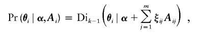where k is the number of subpopulations that underwent admixture, α are the parameters of the Dirichlet distribution that describes the population level admixture, and A_ij is a vector of length k with element i equal to 1 if the locus ancestry is from the ith subpopulation and 0 otherwise.

To reduce the posterior covariance between model parameters and thus ensure rapid mixing of the sampler, each explanatory variable in the regression model is centered about the sample mean; the estimation of these means is performed during the burn-in period. With a linear regression model, the full conditional distribution of the regression parameters is multivariate normal. With a logistic regression model, the full conditional distribution of the regression parameters can be approximated by a normal distribution, which we use as a proposal distribution in a Metropolis-Hastings algorithm. Since the full conditional distribution for the sum-of-intensities parameter τ is log-concave, an adaptive rejection sampler can be used (Gilks and Wild 1992). Autocorrelation beyond 10 iterations is low for all population-level parameters, except for the sum-of-intensities parameter τ. The required number of iterations for burn-in can be kept short by choosing a plausible starting value for this parameter. The current version of the program cannot incorporate prior information about phase, although it samples the joint posterior distribution of ancestry states and haplotypes at each locus.

Appendix B: Posterior Predictive Tests (Bayesian P Values)

Where the alternative to the fitted model cannot be specified as the deviation of a continuous parameter from its specified value, it is possible to construct a test for lack of fit based on the posterior predictive check probability (Rubin 1984). For each realization of the missing data, replicate observations y^rep are generated from the posterior predictive distribution and compared with the observed data y by means of some test statistic T. The posterior predictive check probability is defined as the probability that the value of the test statistic computed from y^rep is more extreme than the value computed from y, , where ω are the model parameters. This probability is evaluated over the posterior distribution of ω and the posterior predictive distribution of y^rep. If there were no posterior uncertainty in ω, this procedure would be equivalent to a classic exact test, in which P values have a uniform distribution on the interval 0–1 in hypothetical repetitions of the experiment when the null hypothesis is true. With posterior uncertainty in ω, the posterior predictive check probabilities are more conservative than classic P values, because their distribution in hypothetical repetitions of the experiment under the null is shrunk toward the expected value of 0.5. Where the test is used as a model diagnostic, rather than for formal statistical inference, this is not a serious problem.

References

- Cavalli-Sforza LL, Menoozz P, Piazzi A (1994) The history and geography of human genes. Princeton University Press, Princeton [Google Scholar]
- Chakraborty R, Weiss KM (1988) Admixture as a tool for finding linked genes and detecting that difference from allelic association between loci. Proc Natl Acad Sci USA 85:9119–9123 [DOI] [PMC free article] [PubMed] [Google Scholar]
- Devlin B, Roeder K, Wasserman L (2003) Analysis of multilocus models of association. Genet Epidemiol 25:36–47 10.1002/gepi.10237 [DOI] [PubMed] [Google Scholar]
- Falush D, Stephens M, Pritchard JK (2003) Inference of population structure using multilocus genotype data: linked loci and correlated allele frequencies. Genetics 164:1567–1587 [DOI] [PMC free article] [PubMed] [Google Scholar]
- Gilks WF, Wild P (1992) Adaptive rejection sampling for Gibbs sampling. Appl Statist 41:337–348 [Google Scholar]
- Hoggart CJ, Parra EJ, Shriver MD, Bonilla C, Kittles RA, Clayton DG, McKeigue PM (2003) Control of confounding of genetic associations in stratified populations. Am J Hum Genet 72:1492–1504 [DOI] [PMC free article] [PubMed] [Google Scholar]
- Jeffreys H (1961) Theory of probability, 3rd ed. Oxford University Press, Oxford [Google Scholar]
- Kilpikari R, Sillanpaa MJ (2003) Bayesian analysis of multilocus association in quantitative and qualitative traits. Genet Epidemiol 25:122–135 10.1002/gepi.10257 [DOI] [PubMed] [Google Scholar]
- Kittles RA, Chen W, Panguluri RK, Ahaghotu C, Jackson A, Adebamowo CA, Griffin R, Williams T, Ukoli F, Adams-Campbell L, Kwagyan J, Isaacs W, Freeman V, Dunston GM, Massac A (2002) CYP3A4-V and prostate cancer in African Americans: causal or confounding association because of population stratification? Hum Genet 110:553–560 10.1007/s00439-002-0731-5 [DOI] [PubMed] [Google Scholar]
- Kittles RA, Panguluri RK, Chen W, Massac A, Ahaghotu C, Jackson A, Ukoli F, Adams-Campbell L, Isaacs W, Dunston GM (2001) Cyp17 promoter variant associated with prostate cancer aggressiveness in African Americans. Cancer Epidemiol Biomarkers Prev 10:943–947 [PubMed] [Google Scholar]
- Kruglyak L, Lander ES (1995a) Complete multipoint sib-pair analysis of qualitative and quantitative traits. Am J Hum Genet 57:439–454 [PMC free article] [PubMed] [Google Scholar]
- ——— (1995b) High-resolution genetic mapping of complex traits. Am J Hum Genet 56:1212–1223 [PMC free article] [PubMed] [Google Scholar]
- Lockwood JR, Roeder K, Devlin B (2001) A Bayesian hierarchical model for allele frequencies. Genet Epidemiol 20:17–33 [DOI] [PubMed] [Google Scholar]
- McKeigue PM (1998) Mapping genes that underlie ethnic differences in disease risk: methods for detecting linkage in admixed populations, by conditioning on parental admixture. Am J Hum Genet 63:241–251 [DOI] [PMC free article] [PubMed] [Google Scholar]
- McKeigue PM, Carpenter JR, Parra EJ, Shriver MD (2000) Estimation of admixture and detection of linkage in admixed populations by a Bayesian approach: application to African-American populations. Ann Hum Genet 64:171–186 10.1046/j.1469-1809.2000.6420171.x [DOI] [PubMed] [Google Scholar]
- Molokhia M, Hoggart C, Patrick AL, Shriver M, Parra E, Ye J, Silman AJ, McKeigue PM (2003) Relation of risk of systemic lupus erythematosus to west African admixture in a Caribbean population. Hum Genet 112:310–318 [DOI] [PubMed] [Google Scholar]
- Mott R, Talbot CJ, Turri MG, Collins AC, Flint J (2000) A method for fine mapping quantitative trait loci in outbred animal stocks. Proc Natl Acad Sci USA 97:12649–12654 10.1073/pnas.230304397 [DOI] [PMC free article] [PubMed] [Google Scholar]
- Parra EJ, Marcini A, Akey J, Martinson J, Batzer MA, Cooper R, Forrester T, Allison DB, Deka R, Ferrell RE, Shriver MD (1998) Estimating African American admixture proportions by use of population-specific alleles. Am J Hum Genet 63:1839–1851 [DOI] [PMC free article] [PubMed] [Google Scholar]
- Rosenberg NA, Li LM, Ward R, Pritchard JK (2003) Informativeness of genetic markers for inference of ancestry. Am J Hum Genet 73:1402–1422 [DOI] [PMC free article] [PubMed] [Google Scholar]
- Rubin DB (1984) Bayesianly justifiable and relevant frequency calculations for the applied statistician. Ann Stat 12:1151–1172 [Google Scholar]
- Sabeti PC, Reich DE, Higgins JM, Levine HZ, Richter DJ, Schaffner SF, Gabriel SB, Platko JV, Patterson NJ, McDonald GJ, Ackerman HC, Campbell SJ, Altshuler D, Cooper R, Kwiatkowski D, Ward R, Lander ES (2002) Detecting recent positive selection in the human genome from haplotype structure. Nature 419:832–837 10.1038/nature01140 [DOI] [PubMed] [Google Scholar]
- Shriver MD, Parra EJ, Dios S, Bonilla C, Norton H, Jovel C, Pfaff C, Jones C, Massac A, Cameron N, Baron A, Jackson T, Argyropoulos G, Jin L, Hoggart CJ, McKeigue PM, Kittles RA (2003) Skin pigmentation, biogeographical ancestry and admixture mapping. Hum Genet 112:387–399 [DOI] [PubMed] [Google Scholar]
- Sillanpaa MJ, Arjas E (1999) Bayesian mapping of multiple quantitative trait loci from incomplete outbred offspring data. Genetics 151:1605–1619 [DOI] [PMC free article] [PubMed] [Google Scholar]
- Stephens JC, Briscoe D, O’Brien SJ (1994) Mapping by admixture linkage disequilibrium in human populations: limits and guidelines. Am J Hum Genet 55:809–824 [PMC free article] [PubMed] [Google Scholar]
- Terwilliger JD, Göring HH (2000) Gene mapping in the 20th and 21st centuries: statistical methods, data analysis, and experimental design. Hum Biol 72:63–132 [PubMed] [Google Scholar]
- Terwilliger JD, Weiss (1998) Linkage disequilibrium mapping of complex disease: fantasy or reality? Curr Opin Biotechnol 9:578–594 10.1016/S0958-1669(98)80135-3 [DOI] [PubMed] [Google Scholar]
- Wright S (1951) The genetical structure of populations. Ann Eugen 15:159–171 [DOI] [PubMed] [Google Scholar]