Methods for High-Density Admixture Mapping of Disease Genes

Abstract

Admixture mapping (also known as “mapping by admixture linkage disequilibrium,” or MALD) has been proposed as an efficient approach to localizing disease-causing variants that differ in frequency (because of either drift or selection) between two historically separated populations. Near a disease gene, patient populations descended from the recent mixing of two or more ethnic groups should have an increased probability of inheriting the alleles derived from the ethnic group that carries more disease-susceptibility alleles. The central attraction of admixture mapping is that, since gene flow has occurred recently in modern populations (e.g., in African and Hispanic Americans in the past 20 generations), it is expected that admixture-generated linkage disequilibrium should extend for many centimorgans. High-resolution marker sets are now becoming available to test this approach, but progress will require (a) computational methods to infer ancestral origin at each point in the genome and (b) empirical characterization of the general properties of linkage disequilibrium due to admixture. Here we describe statistical methods to estimate the ancestral origin of a locus on the basis of the composite genotypes of linked markers, and we show that this approach accurately estimates states of ancestral origin along the genome. We apply this approach to show that strong admixture linkage disequilibrium extends, on average, for 17 cM in African Americans. Finally, we present power calculations under varying models of disease risk, sample size, and proportions of ancestry. Studying ∼2,500 markers in ∼2,500 patients should provide power to detect many regions contributing to common disease. A particularly important result is that the power of an admixture mapping study to detect a locus will be nearly the same for a wide range of mixture scenarios: the mixture proportion should be 10%–90% from both ancestral populations.

Introduction

In the search for disease-causing variants in humans, it is desirable to use whole-genome scans, because they do not require a priori knowledge of the genes involved in disease. The most successful such method to date—linkage analysis in pedigrees—has been very effective at mapping rare disorders for which single mutations are sufficient to cause disease. Linkage analysis has been less successful in localizing risk variants for common, complex disorders, presumably because there are many mutations that contribute to disease, each to a modest degree (Risch and Merikangas 1996; Risch 2000). Attention has therefore turned to association-based approaches, which can provide greater power for identifying common variants conferring modest risk (Risch 2000). The most commonly discussed association approaches are direct association, which requires testing all markers, and haplotype mapping (Collins et al. 1997; Daly et al. 2001; Botstein and Risch 2003). Using either in a whole-genome scan, however, is currently impractical, because both methods require the typing of hundreds of thousands or millions of markers.

Admixture mapping (also known as “mapping by admixture linkage disequilibrium,” or MALD) offers a promising but as yet untested association-based approach for performing a whole-genome scan (Chakraborty and Weiss 1988; Risch 1992; Briscoe et al. 1994; Stephens et al. 1994; McKeigue 1997, 1998; Zheng and Elston 1999; Lautenberger et al. 2000; McKeigue et al. 2000; Wilson and Goldstein 2000; Pfaff et al. 2001; Collins-Schramm et al. 2003; Halder and Shriver 2003; Hoggart et al. 2003; Shriver et al. 2003). The attraction of admixture mapping is that it requires a small fraction of the markers that would be needed for a direct or haplotype scan (∼1% as many) and yet can scan the genome for a subset of risk alleles (those that show substantial differences in frequency between two populations that have recently mixed).

The idea of admixture mapping is simple. Although most genetic variation is shared between groups, some disease-causing variants are known to differ substantially in frequency across populations. This is especially relevant for diseases with different incidences across ethnic groups—for example, autoimmune diseases (usually more common in Europeans) and hypertension and prostate cancer (usually more common in West Africans) (Davey Smith et al. 1998). Admixture mapping is designed to study populations descended, at least in part, from the recent mixing of ethnic groups from multiple parts of the world (such as African Americans and Hispanic Americans). In chromosomal regions containing variants contributing to disease risk, there will be an overrepresentation of ancestry from whichever population has a higher proportion of risk alleles at the locus (fig. 1). For example, multiple sclerosis (MS) is more prevalent in Europeans than in Africans (Kurtzke et al. 1979; Wallin et al. 2003). To identify gene variants that might contribute to the disease, one could screen the genome in African American patients with MS, searching for regions where the proportion of European ancestry is higher (or occasionally lower) than average (fig. 1).

Figure 1.

Schematic of how a disease locus will appear in an admixture scan. Around the locus, there should be an unusually high proportion of ancestry from one of the parental populations, because of patients inheriting high-risk alleles from that group. The peak can be identified not only in a case-control comparison but also in a comparison of the estimate of ancestry in cases at that point in their genome with the rest of their genomes. The width of the peak of association is determined by the number of generations since admixture.

The key advantage of admixture mapping is that, like a haplotype or direct association approach, it is based on directly associating sections of the genome with disease. Thus, for variants that differ strikingly in frequency across populations, it should have more power than linkage to detect the presence of variants of modest effect. At the same time, far fewer genetic markers can be used (a few thousand, rather than 300,000–1,000,000 for a haplotype or direct-association study) (Gabriel et al. 2002; Carlson et al. 2003). Fewer markers are required because admixture has been recent, with <20 generations over which recombination could have broken down segments of shared ancestry. Given the small number of recombination events since admixture, the regions of excess ancestry around disease-causing variants are expected to extend tens of millions of base pairs.

It has only recently become possible to perform high-powered admixture mapping. A powerful study requires a map of thousands of markers known to have substantial differences in frequency across populations. To select these, it is necessary to cull a much larger database of markers with known frequencies. (This is because only a small subset shows high frequency differentiation across groups.) In an accompanying article (Smith et al. 2004 [in this issue]), we present the first high-density, whole-genome map of markers that are useful for admixture mapping in African Americans. This resource is culled from a database of ∼450,000 markers with known frequencies and includes 2,154 well-spaced markers that have been validated as highly differentiated in at least 99 West African and at least 78 European American samples. The markers have an average allele frequency difference of 57% between West Africans and European Americans.

The availability of admixture mapping panels (Smith et al. 2001, 2004) overcomes a major obstacle to performing whole-genome scans by use of admixture-generated linkage disequilibrium. Here, we focus on several additional requirements that must be satisfied to perform a high-powered study. These include (a) developing methods to extract information about ancestry from marker data, (b) characterizing the general properties of admixture-generated LD in an admixed population across the human genome, and (c) understanding how admixture mapping performs under a range of models of genetic effects and allele frequency differentiation among populations.

The article is organized as follows:

• 1. We report a novel method to combine information from multiple, closely linked markers to make local estimates of ancestry. This approach to scanning for disease genes increases power compared with previous proposals, in a manner analogous to multilocus linkage as compared with single-point approaches (Lander and Green 1987).
• 2. We evaluate the performance of the approach on the basis of empirical data collected from African Americans. In the process, we provide the most powerful survey to date of the extent of admixture linkage disequilibrium in African Americans.
• 3. We test the behavior and power of the method through use of extensive computer simulations.
• 4. We explore the power of admixture mapping to detect disease loci under a range of scenarios of genetic effects and allele frequency differentiation, with real and simulated data. These analyses confirm that, for disease-causing alleles with large differences in allele frequencies between the parental populations, admixture mapping can detect genes of modest effect with power comparable to whole-genome haplotype mapping.

We note that Falush et al. (2003) and Hoggart et al. (2003) have developed methods that similarly combine data from multiple, closely linked markers to make inferences about ancestry. When the underlying model is considered, the Falush et al. (2003) method is particularly close to ours, although it aims to infer population structure rather than to scan for disease genes, which has consequences for its implementation. Our method makes advances compared with the others, particularly in the areas of (a) allowing admixture mapping to be applied to the X chromosome, (b) introducing a Bayesian likelihood ratio test to scan for disease association anywhere in the genome, and (c) using adaptive-rejection sampling to allow the software to run more quickly. An additional novel contribution is to present extensive simulation studies showing that the method is robust and not prone to false positives. The simulations show that admixture mapping should, in theory, be able to identify a subset of the genes for complex disease, in some cases with more statistical power than whole-genome haplotype or linkage studies.

The ultimate value of admixture mapping, of course, will depend on whether disease variants that differ strikingly in frequency in populations are common—that is, on the (as yet unknown) frequency distribution across populations of alleles contributing to common disease. This will be determined empirically in the coming years by performing several real admixture mapping studies.

Methods

Here, we present a novel approach for screening along the genome in an individual of recently mixed ancestry, to identify which segments have been inherited from either of the ancestral populations. The estimates can be averaged across individuals to search for an unusual amount of ancestry from one ethnic group, indicating a nearby disease gene.

A Hidden Markov Model (HMM) for Estimating Ancestry along the Genome

We assume that the population under study has recently been derived by the mixing of two populations, A and B, and define the following quantities for each individual:

• M_i = The average proportion of alleles inherited from population A (versus B); for example, for an African American, the proportion of ancestors who lived in Europe before the initiation of admixture—say, >40 generations in the past.
• λ_i = The number of chromosomal exchanges per morgan between ancestral segments of the genome since the mixing event. This includes exchanges between segments of the same ancestry, which are impossible to detect experimentally. This quantity can be roughly identified with the number of generations since the ancestors of individual i began mixing, although this must not be interpreted too literally, since the number of generations since admixture varies across an individual’s different ancestral lineages.

To model how ancestry changes along the genome in an individual, we define the “ancestry state”—that is, whether an individual has 0, 1, or 2 alleles from population A at locus j—as X_j . We denote the sequence of ancestry states at markers 0,1,…,T along a chromosome as X={X₀,X₁,…X_T}. To understand the sequence of ancestry in an individual with a proportion M_i of population A ancestry, we note that, at the p-terminal end of each chromosome, the probability that there are 0, 1, or 2 population A alleles is

Once X_j is specified, the probability distribution of X_j+1 can be calculated as follows. Let d be the genetic distance (in morgans) between markers j and j+1. It is assumed that d is small enough that the probability of two recombination events between markers j and j+1, in any generation, is negligible, which is reasonable for a dense marker map. With probability e^-2λ_id, no recombination occurred between the sites on either chromosome since admixture, and X_j+1=X_j. With probability (1-e^-λ_id)², both chromosomes recombined, in which case X_j+1 can be obtained by drawing from equation (1). With probability 2e^-λ_id(1-e^-λ_id), one chromosome recombined, and X_j+1 can be obtained as a sample average of the two scenarios. The probability of no recombination—and, thus, the same ancestry state—is highest for markers that are close together, corresponding to the fact that markers are much more informative for nearby disease loci (e.g., within 0.5 cM) than for faraway ones (e.g., >5 cM).

The sequence of ancestry states X along the chromosome can be simply represented as a Markov chain on three states in which the transition probabilities vary according to the genetic distance (probability of historical recombination) between markers. The standard way of inferring ancestry states in this situation is by an HMM, in which the ancestry states are “hidden” and must be inferred from the genotypes O={O₀,O₁,…,O_T}, conditional on a model such as the one given above for how the data are generated (Lander and Green 1987; Rabiner 1989; Durbin et al. 1998). The HMM moves from marker to marker along the chromosome (passing through the data twice: once from the p-terminal end and once from the q-terminal end). At each marker, the HMM uses the observed genotypes O and the correlations between nearby markers imposed by the model to produce a probability map for ancestry quantified by α_j(x), β_j(x), and γ_j(x), where x can be 0, 1, or 2 (see appendix A [online only] for details).

The first two quantities (α and β) are the probabilities of x=0, 1, or 2 population alleles inherited from population A at a given marker (j) based on all the data in the p-terminal and q-terminal directions, respectively. To calculate the probability of x population A–ancestry alleles at that point (combining data from both directions), one can then simply multiply α and β together and normalize: γ_j(x)∞α_j(x)β_j(x). The estimates of ancestry (see fig. 2 for examples) can be used directly in tests for association.

Figure 2.

Data from three African American samples (Smith et al. 2004), used to reconstruct ancestry along chromosome 22, based on genotypes at 52 SNPs (the positions of the SNPs are indicated by black lines). Each individual has segments of the genome of both European and African ancestry, randomly distributed over the chromosomes. At any locus, an individual can have only 0, 1, or 2 European ancestry alleles. Individual 3, for example, is confidently estimated to have 1 European-ancestry allele between 0 and 25 cM, 2 between 35 and 40 cM, and 1 between 45 and 70 cM. A higher density of markers is clearly needed to resolve ancestry in some places, highlighting the importance of including more SNPs in the map. To test for disease association on the basis of such data, one would search for genomic segments where the estimated number of European ancestry alleles, summed over samples, is greater than the genomewide average.

It is important to realize that the HMM assumes that M_i and λ_i, as well as the frequencies of alleles in the parental populations, p^A_j and p^B_j, are known. These values are not exactly known in practice, however, and errors in the estimates can lead to false-positive signals of association to disease. In particular, at markers where incorrect parental population allele frequencies are assumed, individuals will appear to be more closely related to one of the parental populations than is, in fact, the case.

To fully take into account uncertainty in the unknown variables, one would ideally run the HMM over all possible combinations of M_i, λ_i, p^A_j, and p^B_j, each time recording the disease association statistic and averaging over all the runs, weighting by their likelihood. However, a typical powerful admixture mapping study might involve 2,500 samples, each with unknown M_i and λ_i, as well as 2,500 markers, each with unknown frequencies p^A_j and p^B_j. It would therefore be necessary to numerically integrate over a grid of 10,000 unknown parameters, which is impossible even with powerful computers. A more sophisticated approach was therefore required to take into account uncertainty in the model parameters.

Markov Chain Monte Carlo (MCMC) Approach

An MCMC approach was applied to account for the uncertainty in allele frequencies and M_i and λ_i. The MCMC makes it feasible to explore the most important parts of a very high-dimensional space of unknown parameters without taking up too much computer time. Instead of methodically integrating over a grid of ∼10,000 dimensions, the MCMC is able to randomly sample from the posterior likelihood distribution of the unknown parameters M_i, λ_i, p^A_j, and p^B_j. Since each iteration of the MCMC is a new sampling from the posterior distribution, by running the HMM and averaging a disease association statistic over the iterations—and performing enough iterations to fully explore the distribution—one can appropriately test for association while taking into account uncertainty in these parameters.

The first step of the MCMC is to pick starting values of the unknown variables.

• 1. The allele frequencies p^A_j and p^B_j are initially set to be the values estimated from the parental populations. For example, in a study of African Americans, a reasonable approach is to estimate the frequencies in European Americans and West Africans.
• 2. The proportion of ancestry M_i is initially set for each individual through use of maximum-likelihood estimates based on treating all SNPs as unlinked.
• 3. The number of generations since admixture, λ_i, is initially set to be 6 (generations) for all samples, on the basis of the empirical estimate for an African American population (see below).

The robustness of the MCMC is not dependent on the initial guesses, since the MCMC will converge to the appropriate posterior distribution regardless of the guess, given a sufficient number of “burn-in” iterations. It is useful to make initial guesses that are reasonably close to the true values, however, because this allows the program to converge more quickly to the correct posterior distribution and reduces computational time.

The main steps of the MCMC, repeated many times, are as follows:

• Step A:

  Use the HMM to randomly generate a sequence of ancestry states across the genome conditional on the current set of parameters p^A_j, p^B_j, M_i, and λ_i.

• Step B:

  Loop over all the ∼10,000 unknown parameters, updating each in turn. For each parameter (e.g., p^A_j or p^B_j for a marker or M_i or λ_i for a sample), its new value is obtained as follows: (i) Hold the values of all other unknowns fixed; (ii) calculate a likelihood distribution for the unknown, conditional on the fixed values of the others (and also on the sequence of ancestry states from step A), and (iii) use this likelihood distribution as a probability distribution for the parameter, randomly sampling from it to obtain an updated value for use in subsequent iterations.

The steps above are typical of modern MCMC analysis in following a “hierarchical Bayesian” framework (Gelman et al. 1995). Such an analysis proceeds in a series of “layers.” In each layer, the conditional distribution of the parameters is generated by the MCMC with the neighboring layers fixed. Most computations then reduce to sampling a single variable with a known likelihood. This is so simple that the main use of computer time is in step A, the sampling of ancestry states by the HMM.

After a sufficient number of “burn-in” iterations (which refers to looping through the full set of ∼10,000 unknown parameters), the MCMC will, to a good approximation, be sampling the correct conditional probability distribution (Gilks and Wild 1992; Gilks et al. 1995, 1996). After burning in, the values of p^A_j, p^B_j, M_i, and λ_i generated by the MCMC can be considered random samples from the true posterior distribution. By performing enough follow-on cycles, one can explore the posterior likelihood surface for these parameters, given the data. In particular, by running the HMM on the particular combination p^A_j, p^B_j, M_i, and λ_i that is generated at the end of each cycle and averaging the disease association statistic over cycles, one can obtain a statistic that appropriately takes into account uncertainty in the unknown parameters. Similarly, one can record the values of each of the unknown parameters p^A_j, p^B_j, M_i, and λ_i at the end of each cycle, building up histograms that approximate these variables’ true likelihood distributions.

We suggest 100 burn-in and 200 follow-on iterations for analysis, since the statistical score for disease association obtained with this procedure is >98% correlated to the score with 1,000 burn-ins and 2,000 follow-ons (see appendix B [online only] for details). It was a surprise to the authors initially that this small number of iterations was sufficient. A likely explanation for the small number of burn-in and follow-on iterations is that, although there are many unknown parameters in the model (∼10,000), the dependence between most pairs of parameters is weak. For example, changing allele frequency guesses for one marker will have little effect on inferences for most others. The required number of burn-in iterations was also minimized by using an expectation-maximization algorithm to pick initial values of the parameters that were relatively close to the true values.

We note four additional and important issues regarding the MCMC approach. First, the software we have written for admixture mapping is, at present, limited to two-way admixture and to diallelic markers (e.g., SNPs).

Second, although controls are not required for a screen for disease genes (the main test for association compares the estimate of ancestry at each locus with the rest of the genome), including control samples can be useful. This is because control samples can provide more-accurate estimates of allele frequencies p^A_j and p^B_j and, hence, more-reliable ancestry inferences at each point in the genome. The “Results” section explicitly explores (using simulations) how useful it is to include controls in a study.

The third feature of the MCMC that was not previously discussed is that the X chromosome has to be analyzed differently from the autosomes. The X chromosome has a different inheritance pattern than the autosomes, and, thus, M^X_i and λ^X_i (the proportion of ancestry and the number of generations since admixture specific to the X chromosome) have to be inferred separately. From empirical data from African American individuals, we observed that M_i and M^X_i are highly correlated in practice, a fact that was used in the MCMC to improve X chromosome inference in this population (appendix B [online only]).

Finally, the MCMC described above does more than account for uncertainty in the estimates of the marker allele frequencies p^A_j and p^B_j due to sampling only a limited number of individuals from populations A and B. In addition, it takes into account the possibility that there may be error in these estimates because the modern samples of A and B that are studied in the laboratory might not be drawn from exactly the same group as the ancestors of the admixed population. The dispersion between the ancestral gene pool of a mixed population and the modern representatives is quantified by two hyperparameters, τ_A and τ_B, which are estimated during the iterations of the MCMC in the same way as M_i, λ_i, p^A_j, and p^B_j (appendix B [online only]) (see Lockwood et al. [2001] and Nicholson et al. [2002] for related measures of population dispersion).

Scoring to Detect the Presence of Disease Genes

Two separate approaches were introduced to formally test the output of the MCMC analysis for the presence of disease genes. The first is a “locus-genome statistic,” which compares the percentage of ancestry derived from one of the parental populations at any locus with the average in the genome (fig. 1). This does not require control samples. The second approach is a “case-control statistic,” which directly compares cases with controls at every point in the genome, looking for differences in ancestry estimates. Both statistics use the outputs of the HMM (γ values). In the context of the MCMC, both statistics are evaluated by averaging the results over the iterations. This appropriately accounts for uncertainty in the unknown parameters p^A_j, p^B_j, M_i, and λ_i, as described in detail below.

Locus-Genome Statistic

The locus-genome statistic compares, for each point in the genome, the likelihood of being a disease locus versus being a locus unrelated to disease. We define ψ₁ and ψ₂ as the increase in disease risk due to having 1 or 2 population A–ancestry alleles, respectively, relative to having no population A–ancestry alleles. It is important to recognize that the risk due to ancestry at a locus is almost always lower than the risk due to a specific allele (since it is an average of both risk and nonrisk alleles at the locus).

The locus-genome statistic is calculated for each individual i separately (and for each marker j in the genome). The statistic is based on the estimated probabilities of 0, 1, or 2 population A alleles for that individual at that point in the genome: γ_i,0(j), γ_i,1(j), and γ_i,2(j), which are provided by the HMM.

The specific test for association is a likelihood-ratio statistic: the likelihood of the data if a disease locus is present divided by the likelihood if no disease locus is present. Theory suggests that this is an optimal statistic (Bickel and Doksum 2001) for detecting evidence of a disease locus. Appendix C (online only) presents some algebra showing that the appropriate likelihood statistic compares the probabilities of 0, 1, or 2 population A–ancestry alleles at a locus based on genotypes there with the expectations based on an individual’s average ancestry as calculated from genomewide data. With η_i,0=(1-M_i)², η_i,1=2M_i(1-M_i), and η_i,2=M²_i,

To obtain the overall likelihood that the locus j is disease-related versus unrelated to disease, one can simply multiply L_ij over all patients (or add log likelihoods and exponentiate). An alternative test for admixture association was introduced by McKeigue et al. (2000).

The locus-genome statistic is flexible enough to test several disease models simultaneously. If one is studying a disease for which there is an epidemiological reason to believe that there is higher genetic risk in population A, one might want to test several models for increased risk due to population A ancestry and, simultaneously (just to be sure), to test one model where population B ancestry confers more risk: for example, ψ₁=1.3, 1.5, 2, and 0.7, with ψ₂=ψ²₁.

An additional attraction of the locus-genome statistic is that it should work well even if the real risk loci do not conform exactly to one of the models being tested. For example, a real locus with ψ₁=ψ₂=2.2 should produce data that are far more likely under the ψ₁=2, ψ₂=4 model than the null (ψ₁=ψ₂=1) hypothesis and thus show up as positive in a scan.

To declare a genomewide significant association to disease—corrected for the fact that multiple loci are being tested—the usual approach is to calculate a statistic at every point in the genome and to declare significance if any locus exceeds a specified threshold (Lander and Kruglyak 1995). The locus-genome statistic, however, also makes it possible to detect evidence for whether there is association anywhere in the genome. The idea is to average the statistic at equally spaced points genomewide (one every cM), declaring a positive association if the log base 10 (LOD) of the average is >2 (appendix C [online only]).

To our knowledge, a Bayesian whole-genome statistic is a novel idea, which could be applied equally well in other contexts (for example, linkage analysis).

Integrating the Locus-Genome Statistic into the MCMC

The previous discussion focused on how to use the results of the HMM to scan for disease genes. To produce a locus-genome statistic that appropriately takes into account uncertainty in the unknown variables p^A_j, p^B_j, M_i, and λ_i, it is appropriate to simply average the locus-genome statistics produced at each iteration of the MCMC.

Case-Control Statistic

The “case-control statistic” compares estimates of ancestry, in cases versus controls, at every point in the genome. A deviation from the genomewide average of one parental population ancestry seen in cases but not controls provides evidence of a disease locus.

Specifically, the case-control statistic calculates, for each individual and every locus j in the genome, the difference between their expected number of population A–ancestry alleles at a locus and the estimate from data: μ_i(j)=2M_i-[2γ_i,2(j)+γ_i,1(j)]. A t statistic (T_j) (Bickel and Doksum 2001) is then calculated for a difference of means μ_i(j) between cases and controls. T_j should be distributed approximately according to a standard normal distribution if there is no disease locus. A useful feature of this statistic is that it internally corrects for population stratification: μ_i(j) should have the same behavior in both cases and controls, even if they have different proportions of population A ancestry, because the average A ancestry is subtracted out for each individual.

The case-control statistic has some advantages compared with the locus-genome statistic. In particular, no explicit risk model is required, so it provides an easier-to-interpret screen for an elevation of ancestry in the parental populations. The case-control statistic also has the advantage that, for prevalent phenotypes such as prostate cancer, hypertension, or response to a drug, it screens for an increase in population A ancestry in cases and a simultaneous decrease in controls selected not to have the phenotype. (The locus-genome statistic, however, can be modified to detect this as well.)

The main drawback of the case-control statistic is that the controls contribute uncertainty to analysis. Thus, an elevation in one population’s ancestry seen in cases may be within the range of statistical fluctuation when taking into account the controls, even though it is statistically significant in comparison with the genomewide average.

Software (in a combination of C and PERL) implementing the MCMC and tests for association is currently being prepared for distribution. This “ANCESTRYMAP” software has been tested only in a Compaq-α Unix environment and is not intended for other computational platforms (a distributable version will be available at the Harvard Medical School Department of Genetics Web site by January 2005, and N.P. or D.R. will assist with analysis of any data sets in the mean time, if requested).

Automatic Checks for Errors in the Data Set

The software includes built-in error checking:

• 1. A “leave1out” program removes the marker contributing the most to any association and assesses whether the signal of association persists. If a signal remains even after leaving out the best marker, it is less likely to be an artifact due to a single marker.
• 2. A “mapcheck” program compares ancestry estimates obtained for each marker by itself to that predicted using adjacent markers (leaving out the SNP of interest). A discrepancy indicates the misspecification of a marker’s genomic position.
• 3. A “freqcheck” program compares the allele frequencies p^A_j and p^B_j observed in the parental populations with those in the mixed population. The mixed population should show appropriately intermediate frequencies at the markers (determined by the genomewide estimates of the proportion of A and B ancestry in that population).

Simulations

Simulated data sets were generated to evaluate the performance of the method:

• 1. For each individual in the simulations, M_i and λ_i are sampled from beta and gamma distributions that are set to match what one might expect in an African American population (M_i∼20%±12%, λ_i∼6±2; see the “Results” section).
• 2. Allele frequencies for the 2,154 markers from the Smith et al. (2004 [in this issue]) map are generated using the statistical model for allele frequencies in appendix B (online only). To model the allele frequency dispersion between the modern populations and the ancestral gene pool of the admixed group, the simulations use τ=300 for both populations A and B, similar to the τ estimates obtained empirically for African Americans with MS (see the “Results” section).
• 3. A Markov chain is used to generate a sequence of ancestral states for each of the chromosomes in a simulated individual. With no disease locus, the simulation proceeds exactly as described in the section on the HMM above. For a disease locus, the algorithm generates an excess of chromosomes under the null (no disease) model and then uses rejection sampling (Ripley 1987) to choose a subset of chromosomes consistent with the presence of a disease locus. Chromosomes with population A ancestry at the disease locus are sampled with probability ψ₁M_i/[ψ₁M_i+(1-M_i)], where ψ₁ is the increased risk for disease due to carrying one population A–ancestry allele.
• 4. Once the allele frequencies and ancestry states at each marker are simulated as described in steps 2 and 3, genotypes can be straightforwardly generated.

In the simulation, the genotypes are separately generated for the chromosomes from each parent, and then the haploid genomes are put together to produce a diploid for analysis.

We also explored how differences in history (M_i and λ_i) for an individual’s two parents can affect power to detect genes. In addition to the simple “scenario 1,” in which the two parents of each individual are simulated to have the same M_i and λ_i, we also considered:

• Scenario 2:

  An individual’s parents are simulated with different ancestry proportions. The parents’ M_i values are generated from a beta distribution with mean and SD that are set to be the same as those measured empirically in African Americans with MS. Some are reassigned to have all A or B ancestry in the right proportion to preserve the mean and variance of M_i in the next generation.

• Scenario 3:

  An individual’s parents are simulated to have different histories of admixture λ_i. The λ_i for each parent is generated from a gamma distribution with a mean and SD in λ_i as in African Americans. A proportion of individuals are then reassigned to have all European or West African ancestry, to preserve variation in λ_i across generations.

Empirical Data to Evaluate the Method

The main data set consists of 756 SNPs (covering 39% of the genome) genotyped in 442 African American patients with MS and 276 African American controls (Oksenberg et al. 2004). The second data set consists of 2,154 SNPs genotyped in 109 African American controls (Smith et al. 2004).

Comparing the Power of Admixture Mapping with That of Other Whole-Genome Scanning Methods

To compare the power of admixture mapping with that of linkage and haplotype mapping, we performed calculations similar to those of Risch and Merikangas (1996) and Risch (2000). We defined power as the number of samples necessary to detect an effect with 80% probability and assumed testing of 300,000 independent hypotheses for the haplotype mapping study. All of these calculations are overoptimistic in terms of the number of samples necessary to detect a disease locus, because they assume a fully informative map for admixture mapping and linkage studies and assume genotyping of the disease risk allele (rather than one in linkage disequilibrium with it) for haplotype studies. In practice, we expect that 1.2- to 2-fold more samples would be required to achieve the claimed level of power.

Results

In the “Methods” section, we presented an approach for estimating the ancestry at each point in the genome in an individual descended from a recent population admixture, through use of genotyping data from closely linked markers. The inputs into this analysis are the genotypes at a large number of genetic variants that are selected as differing strikingly in frequency between two ancestral populations.

The HMM analysis is based on the assumption that the frequencies p^A_j and p^B_j of all the markers in the parental populations are known and that the proportion of ancestry (M_i) and the average number of generations since admixture of populations (λ_i) are also known. In fact, these parameters are uncertain. We therefore used an MCMC approach to account for uncertainty in p^A_j, p^B_j, M_i, and λ_i. The MCMC iterates over a range of possible values of the parameters consistent with the data, averaging results from analyses at the end of each cycle to produce overall estimates.

Finally, we introduced a “locus-genome statistic,” which allows the results of these analyses to be used to test for the likelihood of the data given the presence of a disease-influencing gene (as compared with the absence of such an allele). The locus-genome statistic compares the estimates of ancestry for each individual at each locus with the average genomewide (M_i), searching for a deviation that indicates the presence of a disease gene (fig. 1). The statistic is efficient at extracting nearly all information about disease association (see below). We also introduced a statistic that conventionally searches for a difference between cases and controls at each locus.

The “Results” section is organized in three parts:

• 1. We assess the performance of the MCMC through use of empirical data sets. This provides a rigorous assessment of the extent of admixture-generation linkage disequilibrium and the proportion of European ancestry in African Americans.
• 2. We assess the robustness and performance of the MCMC through use of simulated data sets, showing that the method can detect associations, is not prone to false positives, and has the high statistical power to detect disease genes that is expected theoretically.
• 3. We present power calculations comparing admixture mapping with other methods. In the process, we suggest guidelines for the design of admixture genome scans.

Performance of MCMC on Real Data

The analysis can scan along the genome of an individual estimating ancestry

In figure 2, we show the output of the analysis based on genotyping data from three African American individuals. The plots focusing on chromosome 22 show clear transitions between 0, 1, or 2 European-ancestry alleles.

The MCMC can detect regions of elevated European ancestry in African Americans

To evaluate the performance of the method, we examined a large data set consisting of 442 African Americans with MS and 276 controls, genotyped at 756 SNPs covering 39% of the genome (to be fully described elsewhere).

We began by identifying five polymorphisms with large frequency differences between West Africans and European Americans. From the 442 patients in the study, we selected a subset carrying the genetic variant that was relatively more common in Europeans. These individuals were expected to have an elevated proportion of European ancestry at that locus. Figure 3 shows that the MCMC successfully detects these loci (without including the genotypes of the marker used to select the locus). The LOD scores range between 4 and 15, indicating 10⁴:1 to 10¹⁵:1 odds of seeing a result so extreme by chance. Strong admixture linkage disequilibrium covers a region 10–20 cM around each locus. These results are comparable to the high admixture-generated LD in African Americans measured around FY (Parra et al. 1998; Lautenberger et al. 2000; McKeigue et al. 2000).

Figure 3.

Quantitative assessment of the ability of the MCMC to detect regions of the genome with high or low levels of European ancestry. From the 442 patients with MS, we identified subsets of individuals carrying at least one copy of an allele that has a much higher frequency in Europeans than in Africans, thereby defining five populations that we knew were enriched for European ancestry at that point in their genomes. For the analyses, we conditioned on genotypes at the following five polymorphisms: DRB1*1501 in human leukocyte antigen (HLA) (n=57 individuals), rs7349 (n=125), rs1002587 (n=129), rs1205817 (n=177), and rs737802 (n=141). We tested for association through use of the locus-genome statistic and a disease model of twofold increased risk due to European ancestry (ψ₁=2; ψ₂=4). Peaks of highly significant ancestry association were identified in all five examples, with widths of 10–15 cM (where the width is defined as the log likelihood being within 1 of the maximum). Positions of the highly informative markers used for inference are indicated by triangles at the bottom of each figure.

Estimates of genomic parameters relevant to admixture mapping in African Americans

With the large MS cohort sample, we were able to obtain rigorous estimates of the proportion of European ancestry and the extent of admixture-generated linkage disequilibrium in African Americans. The overall proportion of European ancestry in the 718 samples was M_i=21%, slightly higher than the 15%–20% estimates in previous studies of African American populations (Parra et al. 1998). The per-individual estimates from our MCMC agree closely with estimates from a maximum-likelihood analysis (fig. 4A) and the STRUCTURE program (Falush et al. 2003) (data not shown). We were also able, for the first time, to precisely estimate the variability of ancestry proportion across African Americans: M_i∼21%±11%. This is important in disease studies, since individuals with <10% ancestry from one parental population provide much less power (see below).

Figure 4.

A, Estimates of percent European ancestry for 718 African American individuals, based on empirical data collected at our laboratory. We compare the estimates of ancestry from the MCMC with estimates made through use of a simple maximum-likelihood approach using a subset of 186 unlinked markers that were chosen to have the highest information content (Smith et al. 2004 [in this issue]) while spaced at least 10 cM apart. The close correlation provides confidence that the MCMC accurately estimates unknown parameters. B, Comparison of M_i with λ_i estimates (the SEs are shown in gray). Individuals with high M_i often have low λ_i values, which may be due to these individuals often having one European parent, resulting in an M_i near 50% but a low λ_i because the chromosome from the European parent never crosses over. Such individuals should ideally be excluded from an African American admixture mapping study (i.e., samples' parents should not have entirely European American or West African ancestry), because chromosomes that do not cross over between ancestries contribute no power to a study.

The other important parameter in admixture mapping is the average number of generations since admixture (fig. 4B). We estimate λ_i=6.0, on average, but note that this is somewhat difficult to interpret, because the number of generations since admixture is different on every lineage in a person’s ancestry. The inverse, 1/λ_i, however, is the average extent of strong admixture-generated LD in African Americans (1/λ_i=17 cM). Falush et al. (2003) estimated 1/λ_i=10 cM, and Collins-Schramm et al. (2003) estimated 10–20 cM in different genomewide data sets in different population samples.

Third, the MCMC analysis allowed us to assess how closely the West African and European American populations corresponded to the true parental populations for African Americans. The algorithm estimates a parameter—τ_A for Europeans and τ_B for Africans—indicating how much drift has occurred between the parental population and actual European American and West African samples that had been genotyped. An interpretation of τ_E and τ_A is that the true frequencies in the parental populations of African Americans are as close to those in the European American and West African controls as would be expected if the control sample frequencies were obtained by sampling τ_A alleles and τ_B alleles from the ancestral African American populations (Nicholson et al. 2002). The West African and European Americans are fairly close to the parental populations (τ_A=430±76 and τ_B=253±59, corresponding to F_st values of 0.001 and 0.002, respectively, using the formula relating τ to Wright’s F_st from Lockwood et al. [2001]: ).

Evaluating the performance of the computer software

We ran the MCMC analysis on several data sets. The analysis ran in 40 min on the MS data set (756 SNPs and 718 samples), in 12 min on a subset of the map data set (2,147 SNPs and 109 samples [Smith et al. 2004]), and in half a minute on a previously published data set (33 SNPs and 235 samples [Hoggart et al. 2003]). Simulation studies showed that the speed increases approximately linearly with the number of SNPs and samples. For example, on a simulated data set of the size that is likely to be used in powerful admixture mapping studies (2,147 SNPs in 2,000 samples), the program ran in 222 minutes. Thus, the program is sufficiently fast that it is practical to analyze genomewide data sets in large patient samples. The high speed also allowed us to perform extensive power calculations and thorough debugging of software, which is important for a large MCMC such as ours, since such programs have few internal checks.

Assessing the Performance of the MCMC by Computer Simulation

Simulations to assess the robustness of the method in estimating unknown parameters

To evaluate how well our estimates of p^A_j, p^B_j, M_i, and λ_i correspond to their true values, we generated simulated data sets in which the true values of the parameters were known. As shown in the simulations in figure 5, the estimates produced by the MCMC are unbiased, with about an equal number positive and negative. Even with deviations from our model assumptions (scenarios 2 and 3 in the “Methods” section), λ_i is underestimated by no more than 7%, on average (table 1), which is not enough to cause false positives.

Figure 5.

Difference between the true values of M_i, λ_i, p^A_j, and p^B_j and the estimates from the MCMC. These results are obtained by simulating data sets in which 1,000 samples are genotyped in 2,147 markers from the map described by Smith et al. (2004 [in this issue]). In the simulations, we set M_i=20%±12% and λ_i=6±2, to match the values observed empirically in African Americans, and we assume no disease locus. The difference between the true value and estimate (divided by the estimated SE estimated by the MCMC) is, on average, close to 0, indicating that the estimates are unbiased. Compared with normal theory, the residuals are larger than expected, indicating that the MCMC slightly underestimates the SEs, although this does not appear to cause false positives (table 2).

Table 1.

Accuracy of MCMC Parameter Estimates^[Note]

Scenario	Mi (DispersionCompared withNormal Theory)a	λi (DispersionCompared withNormal Theory)a	Residual of pAj and pBj (Dispersion Compared with Normal Theory)b
Null model (scenario 1) (see also fig. 5)	20.0% (2.1-fold)	6.0 (2.0-fold)	−.02 (2.1-fold)
Mi varies between parents (scenario 2)	19.9% (1.9-fold)	5.6 (10.7-fold)	−.01 (2.0-fold)
λi varies between parents (scenario 3)	19.6% (2.3-fold)	5.8 (2.3-fold)	−.02 (2.0-fold)

Note.— We assessed how well the MCMC estimates unknown parameters by performing simulations of 1,000 individuals without disease studied at 2,147 markers from the map described by Smith et al. (2004 [in this issue]). The simulations assume that the samples have percentages of European ancestry with distributions of M_i∼20%±12% and λ_i∼6±2 generations. The frequencies of the markers are based on the West African and European American frequencies from the Smith et al. (2004 [in this issue]) map. The data for simulations of admixture conforming fully to our model are presented in the first row (and pictorially in fig. 5). The means of both M_i and λ_i are within 7% of their true values even in the presence of large deviations from the model, and the allele frequency estimates are essentially unaffected by deviations from the model. The dispersions (measuring the spread of the residuals around the mean) are generally more than twice the values expected from normal theory. This indicates that the MCMC is overconfident about its parameter estimates. However, this does not appear to increase the values of disease association statistics, and, hence, it would not be expected to lead to false positives (table 2).

^aValues for M_i and λ_i are averaged over 1,000 individuals (if estimates are unbiased, they should be M_i=20% and λ_i=6 generations).

^bValues for p^A_j and p^B_j are the mean residuals (the difference between the true and estimated value, divided by the estimated SE) out of 2,147 × 2 frequency estimates; should be ∼0 if unbiased.

Simulations to assess the distribution of statistics in the absence of a disease locus

We performed a series of 100 simulations to assess how association statistics behave in the absence of a disease locus (that is, to generate a null distribution). The 95th percentile is −0.1 for the whole-genome score (table 2) for a simulated scenario of 200 African American samples genotyped at the 2,147 markers from the Smith et al. (2004 [in this issue]) map. We note that the 95th percentile can change depending on the disease model. Thus, we recommend not declaring genomewide significance if the LOD score is <2, unless simulations are performed that mimic the structure of the data set. The threshold for genomewide significance does not change even if M_i and λ_i differ across the parents of individuals in a study (scenarios 2 and 3 in the “Methods” section) (table 2). Thus, the test for association appears robust to substantial deviations from model assumptions.

Table 2.

The 95th Percentiles of Association Statistics in the Absence of a Disease Locus (These Translate Directly to Thresholds for Genomewide Significance)^[Note]

	95th Percentile
Scenario	Locus-Genome Statistic (Whole-Genome Score)	Locus-Genome Statistic (Strongest Marker in Genome)	Case-Control Statistic (Strongest Marker in Genome)
Null model (scenario 1)	−.1	2.7	3.7
Mi varies between parents (scenario 2)	−.3	2.4	3.7
λi varies between parents (scenario 3)	.1	2.8	3.7
Disease locus (2-fold increased risk due to ancestry)a	.3–7.3	2.3–10.4	2.7–5.5

Note.— We performed 100 simulations with no disease locus for each of the three scenarios described in the text, for 200 cases and 200 controls with M_i∼20%±12% and λ_i∼6±2 studied in 2,147 of the markers described by Smith et al. (2004 [in this issue]), and analyzed the data with the disease association statistics. The 95th percentiles of simulations in the absence of a disease locus are approximately the same whether or not M_i and λ_i vary between parents. This indicates that substantial deviations from model assumptions are not likely to cause false positives in the MCMC analysis. For comparison, we also present simulations based on a real disease locus (twofold increased risk).

^aValues in this row are 5th–95th percentile ranges.

Simulations to assess statistical power to detect a disease locus

We simulated disease loci where inheriting alleles from population A confers 1.3-, 1.5-, 1.7-, and 2-fold increased risk compared with population B (fig. 6) (we assumed ranges of M_i and λ_i similar those in to African Americans). It is important to realize that these risk factors differ from the genotype relative risk (GRR)—the risk due to inheriting one copy of an allele—that are quoted in most power calculations. What is relevant to admixture mapping is the risk averaged over all alleles at a locus in population A compared with the risk averaged over all alleles in population B. Since the risk is averaged over risk and nonrisk alleles, the risk due to ancestry is usually less than the GRR.

Figure 6.

Simulations to assess the power of the method to detect a disease locus at which a population A–ancestry allele confers 1-, 1.3-, 1.5-, 1.7-, and 2-fold multiplicative increased risk. The ancestry of the samples was assumed to be M_i∼20%±12% and λ_i∼6±2, and the markers are 2,147 from the map described in the accompanying article by Smith et al. (2004 [in this issue]). For the simulations, we picked a “typical” locus from the map (chromosome 8, position 131 cM), where the estimated information about ancestry provided by nearby markers (estimated as described by Smith et al. 2004 [in this issue]) is 67% of the maximum. For each of the five risk models and sample sizes of 250, 500, 750, 1,000, and 2,000 (assuming equal numbers of cases and controls), 20 simulations were performed. The number of simulations that pass the genomewide threshold of significance (LOD >2) was plotted for the main locus-genome statistic (we used a hypothesis of equally likely risk models of ψ₁=0.5, 1.3, 1.5, and 2.0, with ψ₂=ψ²₁ in the locus-genome tests for association). These simulations demonstrate that even relative risks due to ancestry of as little as 1.3 can be detected by admixture mapping with 2,000 cases and controls. The significance threshold we use (LOD >2) is quite stringent, so, in practice, many simulations that do not formally exceed this significance threshold will produce large enough scores (LOD >0) that they would be followed up by studying a higher density of markers at the strongest peaks of association. Extraction of substantially more information by genotyping a higher density of markers should bring real disease loci above the genomewide threshold of significance.

We found that (a) 250 samples provided high power (60%) to detect 2-fold risk due to ancestry, (b) 500 samples provided high power (70%) to detect 1.7-fold risk due to ancestry, (c) 1,000 samples provided high power (95%) to detect 1.5-fold risk due to ancestry, and (d) 2,000 samples provided high power (75%) to detect 1.3-fold risk due to ancestry.

Simulations to assess how map quality affects power

The power of admixture mapping is strongly dependent on the quality and density of markers in the map, which changes from position to position in the genome (McKeigue 1998; McKeigue et al. 2000). In an accompanying article (Smith et al. 2004 [in this issue]), we describe a map for African Americans based on 2,154 SNPs, 2,147 of which are used in all the simulations discussed here. The average information content is estimated to be 71% in that article; however, that calculation does not take into account uncertainty in the allele frequencies. Our simulations show that the true average is closer to 50% (fig. 7), comparable to current standard linkage maps (M.J.D., unpublished data). This means that, to detect a disease locus with a given probability of success, one would need to study about twice the samples as would be required in the “ideal” scenario of studying an infinitely dense and maximally informative map of markers (fig. 8).

Figure 7.

Effect of map quality on the power to detect a disease locus. Using the 2,147 markers from the map described by Smith et al. (2004 [in this issue]), we performed 100 simulations with 200 cases and 200 controls and a multiplicative risk model of 2 due to a European-ancestry allele. We performed the simulations for six loci where the information extractions, according to our theoretical calculation (described in detail by Smith et al. 2004 [in this issue]), were 0.5, 0.6, 0.7, 0.8, 0.9, and 1. The inverse of information extraction should be the same as the increase in sample size that is necessary to detect a disease locus there (as compared with perfect information). For example, at the Duffy locus on chromosome 1—the rightmost data point in this figure—an allele distinguishes essentially perfectly between West African and European ancestry, and information extraction is 1. Our simulations show that genomewide scores, in practice, increase faster than would be expected on the basis of the theoretical power calculation (dashed line). Thus, although the average locus in the map has claimed 71% information extraction, the mean association score from simulations is ∼50% of the Duffy locus. The power loss compared with theory is due, we believe, to the fact that there is less certainty about allele frequencies at loci where there is lower information extraction, so the MCMC is less certain about declaring an association.

Figure 8.

Comparison of the power of sib-pair linkage mapping, haplotype association mapping, and admixture mapping. A, Power as a function of sample size. These charts present the number of case-control or sib-sib pairs that are expected to be required to detect a disease locus. To set thresholds for genomewide significance, we assume that 300,000 independent markers have been tested for haplotype mapping (including the real risk allele) and that there is perfect information extraction for linkage and admixture mapping, with all samples having a proportion of population A ancestry (for example, European ancestry in African Americans) of M_i=20%. These represent idealized scenarios, so that, in practice, 1.2- to 2-fold more samples would be required than are shown here (see the “Methods” section). For simplicity, we assume that the allele that is being studied is the only one at the locus that increases risk for the disease (with all other alleles conferring equal and lower risk). These results show that, for low-penetrance risk alleles (1.3-fold, 1.5-fold, and 2-fold increased risk due to the allele rather than ancestry) that differ substantially in frequency across populations, admixture mapping requires many fewer samples than linkage mapping (although usually more samples than haplotype-based association mapping). B, Power as a function of number of genotypes. These charts correspond to the same scenarios but report the number of genotypes required rather than the number of samples. The advantages of admixture mapping are most apparent in this comparison, since many fewer markers are required for a whole-genome admixture scan than a whole-genome association scan.

We advocate studying a much higher density of markers (and more samples) than the 200–300 markers (and 200–300 cases and controls) suggested by Stephens et al. (1994) in their original admixture mapping power calculations. Stephens et al. (1994) suggested studying fewer samples because they were investigating power for a phenotype for which the penetrance in families is high. Since family-based (linkage) studies are highly efficient in this situation, admixture mapping has no comparative advantage in this case. Admixture mapping will have the greatest advantage, compared with linkage mapping, for late-onset complex traits for which heritabilities are low, a situation in which the statistical signal is weaker and therefore more samples are required.

Simulations assessing the value of control samples in a study

Admixture mapping differs from other association approaches in that it can, in principle, be performed as a case-only analysis. This is because the proportion of ancestry at each locus can be compared with the genomewide average (fig. 1). In practice, however, the inclusion of control samples can improve power by providing more certainty about allele frequencies in the ancestral populations. This raises two questions. First, which is better: controls from the mixed population or from the parental populations? Second, how many controls should be examined?

To assess how useful controls are in an admixture mapping study, we performed simulations with 200 cases and different numbers of controls, for a locus conferring twofold increased risk of disease. In these simulations, controls add only a small amount of information compared with that provided by genotyping 78 European American and 99 West African samples for the Smith et al. (2004 [in this issue]) map. In a series of 100 simulations with a 2-fold increased risk locus, the average LOD scores for association were 1.88, 1.95, and 2.15 for 0, 200, and 2,000 controls, respectively. Increasing the number of cases to 2,000, by contrast, confers far more power than increasing the number of controls by the same amount: the average LOD score for association is 5.06 even in the presence of a much weaker (1.5-fold) increased risk locus.

We conclude that, in designing an admixture mapping study, one should make the collection of cases as large as possible, with the size of the control population a secondary objective. A minimum of a few hundred control samples should probably be included in any disease study as a sanity check, to ensure that any signals of admixture association are restricted to cases and not seen in controls. Admixed control samples will also likely be more important for studies in populations such as Hispanic Americans than in African Americans, since, in Hispanic Americans, it may be more difficult to identify modern representatives of the actual parental populations, and the only reliable source of allele frequency information will be admixed control samples.

Theoretical Power Calculations, and Guidelines for Optimal Study Design

We performed power calculations for admixture mapping under a very wide range of disease models, assuming a perfectly informative map. The results should apply equally to any approach to admixture mapping (McKeigue 1997, 1998; Zheng and Elston 1999; McKeigue et al. 2000; Hoggart et al. 2003), and not just to our own.

Theoretical power of admixture mapping to detect known disease loci

To explore the theoretical power of admixture mapping—what would be expected if our genetic methods were perfect and we genotyped perfectly informative sites at every point in the genome—we first explored the power of admixture mapping to detect genetic variants that have been associated with common, complex diseases (Hirschhorn et al. 2002; Lohmueller et al. 2003).

For each of the examples presented in table 3, we used published data about the relative frequencies of the alleles in Europeans and West Africans, as well as the relative risk due to carrying 1 or 2 copies of the allele, to estimate the increased risk due to ancestry at the locus.

Table 3.

Number of Samples Required by Admixture Mapping versus Linkage and Direct Association Studies to Detect Known Risk Alleles^[Note]

		Increased Risk		Frequency in(%)		Increased Risk for		No. of Samples Requiredfor 80% Power in
Locus (Allele)	Phenotype	Due toHeterozygosityfor Risk Allele(ψ1)	Due toHomozygosityfor Risk Allele(ψ2)	Europeans	WestAfricans	1 European-AncestryAllele	2 European-AncestryAlleles	AdmixtureMapping	HaplotypeMapping	LinkageMapping
CTLA4 (Ala allele in Thr17Ala)a,b	Type I diabetes	1.26	1.74	38	21	1.04	1.08	36,144	2,557	233,169
INS (class I allele in VNTR)c,d	Type I diabetes	2.30	2.86	71	23	1.48	2.19	974	448	8,203
DRD3 (Ser allele in Ser9Gly)b,e	Schizophrenia	1	1.12	67	12	1.01	1.05	346,816	265,999	380,983,674
AGT (Thr allele in Thr235Met)f,g,h	Hypertension	1.12	1.31	42	91	.93	.87	16,034	11,332	4,941,111
PPAR-γ (Pro allele in Pro12Ala)b,i	Type II diabetes	1.3	1.7	85	100	.97	.93	62,134	21,297	18,151,737
CTLA4 (Ala allele in Thr17Ala)c,j,k	Graves disease	1.32	1.80	38	21	1.05	1.10	28,861	2,041	157,555
PRNP (Met allele in Met129Val)c,l,m	CJD susceptibility	1.88	3.57	72	56	1.11	1.23	9,081	422	7,666
APOE (E4 allele)c,n,o	Alzheimer disease	4.2	14.9	14	30	.76	.57	1,165	71	316
F5 (Leiden allele)c,p,q	Venous thrombosis	7.83	80	4	0	1.27	1.62	1,156	134	457
IBD5 (A allele in IGR2096a_1 A/C)r,s,t	Inflammatory bowel disease	1.38	2	35	0	1.13	1.30	4,596	3,918	565,369
KCNJ11 (Lys allele in Glu23Lys)u	Type II diabetes	1.12	1.47	34	3	1.02	1.05	43,312	22,466	15,589,550
HLA DR2 (DRB1*1501)v	Multiple sclerosis	2.7	6.7	11	0	1.19	1.40	2,498	678	16,047
ABCB1 (C allele in C3435T)w	Epilepsy treatment	1.47	2.66	50	10	1.20	1.50	1,985	969	30,623
GNB3(T allele in C825T)x	Obesity (BMI >27)	1.98	3.59	30	81	.75	.55	1,055	602	15,704
β-globin (Val allele in Glu6Val)y	Sickle-cell disease	1	1,000	0	6	.22	.22	92	5	14

Note.— To estimate the increased risk due to 1 or 2 European ancestry alleles, we used the frequencies of the risk alleles in European and West Africans and the increased risk due to one or two copies estimated in European Americans. For calculating the power of linkage analysis and admixture mapping, we assumed fully informative maps, and assumed 300,000 independent hypotheses for direct association studies. The first nine lines in the table show associations with complex disease identified by Hirschhorn et al. (2002), Lohmueller et al. (2003), and K. Lohmueller (unpublished data) that were significant in meta-analysis or reproducible in 75% of follow-up studies (with the caveat that their frequencies were available in Europeans and Africans). The odds ratios are calculated from follow-on studies, where increased risk due to heterozygosity was estimated using the odds ratio for the risk allele rather than the heterozygous genotype. Lines 10–14 show less well-established associations with complex disease, and line 15 shows a Mendelian disease.

^aOsei-Hyiaman et al. 2001.

^bLohmueller et al. 2003.

^cHirschhorn et al. 2002.

^dPermutt and Elbein 1990.

^eCrocq et al. 1996.

^fRotimi et al. 1996.

^gNakajima et al. 2002.

^hK.E.L., unpublished data.

ⁱAltshuler et al. 2000.

^jUeda et al. 2003.

^kDonner et al. 1997.

^lMead et al. 2001.

^mSoldevila et al. 2003.

ⁿFarrer et al. 1997.

^oCorbo and Scacchi 1999.

^pRosendaal et al. 1995.

^qRees et al. 1995.

^rRioux et al. 2001.

^sGiallourakis et al. 2003.

^tM.J.D., unpublished data.

^uD.A., unpublished data.

^vBarcellos et al. 2003.

^wSiddiqui et al. 2003.

^xSiffert et al. 1999.

^yHill et al. 1991.

It is interesting that only a few of these known variants would have been detectable with high power through use of admixture mapping. This is because the method will work only for the subset of risk variants that differ strikingly in frequency across populations, and it is not yet clear how important these are in human disease. We emphasize that, since admixture mapping was not used to identify the variants in table 3, the table has a bias toward alleles that will not be amenable to admixture mapping.

The prospects of admixture mapping are likely to be best for diseases, such as MS and prostate cancer, with sharply different incidences across populations. For such diseases, there is a higher probability that the genetic risk is due to alleles that have very different frequencies across populations. The true usefulness of admixture mapping will only be clear once several real, empirical, high-powered studies are performed for diseases that differ strikingly in incidence across populations.

Theoretical exploration of power of admixture mapping for a range of disease models

To more fully explore how admixture mapping compares in power with other whole-genome scanning approaches, we performed theoretical calculations comparing the power of admixture mapping with that of linkage studies and of whole-genome association mapping. The calculations we used for the latter two methods are similar to those described by Risch and colleagues (Risch and Merikangas 1996; Risch 2000). Figure 8A shows that an admixture mapping study involving a high-density map of markers in African Americans should, in many cases, have statistical power similar to that of a whole-genome haplotype or association study and should require fewer samples than a linkage scan to achieve the same statistical power. Admixture mapping works well, of course, only for alleles with a large allele frequency difference across populations.

The high efficiency of admixture mapping is most evident when one focuses on the number of genotypes required for a study (fig. 8B). The reason is that admixture mapping requires genotyping ∼100 times fewer markers than haplotype mapping but retains the high power of an association study. The power calculations in figure 8 suggest that, with 2,000 samples and a high-density map, it should be possible, in principle, to use admixture mapping to detect disease loci where the relative risk due to an allele (the GRR, not the ancestry risk) is as low as 1.5.

Power is affected by proportion of ancestry

In the extreme case, an individual with ancestry solely from one population (M_i=0 or 1) shows no crossovers between segments of different ancestry and thus contributes no power for a study. However, figure 9 also shows that power is fairly constant for values of M_i from 10% to 90%. Since the average proportion of European ancestry is 15%–21% for African American populations (Parra et al. 1998; present study) and is estimated to be 53%–68% for Hispanic American populations (Halder and Shriver 2003), we conclude that both African and Hispanic Americans are in the range of mixture proportions where admixture mapping should have high power.

Figure 9.

Number of samples required to detect a disease locus where population A ancestry, on average, increases risk, as a function of the proportion of ancestry in each sample. Individuals with population A ancestry between 10% and 90% provide the most power. The power for admixture mapping contributed by a typical African American sample (20% European ancestry; 80% African ancestry) corresponds to a percent population A of 0.2 (European ancestry confers increased risk) or 0.8 (African ancestry confers increased risk). Fewer samples are required if the less common (European) ancestry confers increased risk (e.g., a disease such as MS rather than prostate cancer), although the effect is slight (only 1.2- to 1.3-fold more samples are required to achieve the same power; see fig. 10). We note that this graph assumes perfect information extraction and the same M_i for the two parents of each sample. Deviations from these assumptions—in particular, the imperfect information extraction in real maps such as that described by Smith et al. (2004 [in this issue])—mean that the number of samples required for a practical study would be about twice as high as shown.

The identity of the ancestral population with higher risk at a locus only modestly affects power

It has been previously noted that it should be easier to detect a locus if the increase in ancestry is from the population contributing less to the admixed population. To assess the importance of this effect, we integrated the power calculations (fig. 9) over the distribution of percent European ancestry (M_i) in African Americans (fig. 10).

Figure 10.

Number of samples necessary to detect a disease locus under the ideal assumption of perfect information about ancestry and the same M_i in both parents. The number of samples necessary to detect an association in African Americans is estimated by averaging the power for a given risk model and percentage of ancestry (given by the curves in fig. 9) over the percentages of ancestry seen in African Americans: M_i∼20%±12% as described in the text.

These calculations show that, for loci where African ancestry confers higher risk (which might be expected in prostate cancer), the power is only slightly lower than for loci where European ancestry confers higher risk (expected for diseases like MS). For example, if African Americans are assumed to have 20% European admixture on average, and if we consider a 1.5-fold relative-risk allele that has frequencies of 10% in European Americans and 60% in West Africans, we expect that 1,925 samples would be needed to detect it with 80% power. The sample requirement would be reduced by only 1.24-fold if the population frequencies were reversed. We conclude that the power of admixture mapping is affected little by which ancestral population has a higher incidence.

Theory suggests that performance is affected by the number of generations since admixture

The number of generations since admixture also has an impact on power to detect a disease locus. For patients with a recent history of admixture (low λ_i, which could occur if all four grandparents were from unadmixed populations) the sizes of blocks of shared ancestry should be large, and fewer markers should be necessary to provide high confidence about their ancestry state (0, 1, or 2 population A alleles). The drawback of a low λ_i, however, is that, once a peak is detected, there will be less precision in localization.

Discussion

We have described a new method that allows genotyping data from closely linked markers to be combined to permit robust, powerful, and practical admixture scans for disease genes. We have also verified that the method works well, through use of empirical and simulated data. Finally, we have performed power calculations that should be relevant not only to the method we introduced but also to other admixture scanning methods. We emphasize that admixture mapping will be useful only if it is combined with a robust panel of markers specifically chosen for admixture mapping. Thus, in an accompanying article (Smith et al. 2004 [in this issue]), we also present a high-density admixture map containing 2,154 SNPs, which, for the first time, should make it practical to use the admixture mapping method as a disease gene scanning method in African Americans.

It is important to recognize that, although admixture mapping is a promising approach, it can only map variants contributing to common disease that show large allele frequency differences between parental populations. Ideally, several methods will be used in conjunction with one another to find as many risk variants as possible:

• 1. Linkage mapping or homozygosity mapping are always the most powerful and cost-effective approaches for identifying disease genes for which the penetrance in families is high.
• 2. Haplotype mapping or direct association studies have the virtue that they can identify common alleles of low penetrance. However, whole-genome haplotype scans require the study of so many markers that they will not be practical until costs decrease. At present, the only practical haplotype studies are of specific candidate regions.
• 3. Admixture mapping is an alternative approach to whole-genome scans for low-penetrance risk variants for common disease. It will work best for finding loci where the genetically influential disease risk differs across populations. This may be most important where natural selection has altered the allele frequency in different groups.

Admixture mapping is likely to be most promising for diseases in which incidence differs strikingly across populations, since these differences may signal the existence of alleles that also differ in frequency across populations. (Of course, environmental influences and sociocultural factors also explain many health disparities between populations.) It is important to realize, however, that admixture mapping is not limited to phenotypes that differ in incidence across populations. Even for populations in which the incidence is the same, the genetic risk factors may be differently distributed across loci, so that an admixture study would detect them as regions of both increased and decreased ancestry.

Admixture mapping can be tested in practice only by performing several real empirical studies. We conclude that, even if the method works as well as theoretically predicted, it is not a replacement for haplotype-based mapping. At loci where peaks are detected, regions of interest will span multiple centimorgans, and haplotype-based approaches will be crucial for fine-mapping the peaks and cloning the disease gene.

Appendix A: The HMM as Applied to Admixture Mapping

For an individual i, M_i is defined as the individual’s genomewide proportion of population A ancestry, and λ_i is defined as the mean number of crossovers per morgan between ancestral sequences in the individual’s genome.

Along a particular chromosome, we are studying T+1 markers sorted in the 5′ to 3′ direction, identified by the variable j∈{0,1,…,T}. The individual’s genotypes for this chromosome are represented as a sequence of observations O={O₀,O₁,…,O_T}, where O_j∈{0,1,2} denotes the number of copies of a reference allele that are carried at locus j. The frequency of the reference allele for marker j in population A is denoted by p^A_j; the frequency in population B is p^B_j.

The “hidden” variable in the HMM analysis is the sequence of ancestry states X={X₀,X₁,…,X_T}, where X_j∈{0,1,2} is the number of alleles deriving from population A ancestry at locus j. With the above parameters as inputs in the HMM, we calculate the likelihood of the data as well as the posterior probabilities of the ancestry state X_j at each site.

We note that our alpha-pass and beta-pass algorithms are extremely similar to the Lander-Green algorithm (Lander and Green 1987) and to algorithms described by Falush et al. (2003). They are specializations of methods introduced by Baum (Baum et al. 1970).

Alpha Pass

We begin at the p-terminal end of the chromosome and proceed iteratively in the 5′ direction. At marker 0, we define our prior probability for the ancestry state: α^*₀(x)=P(X₀=x), where x∈{0,1,2}. Explicitly, this is α^*₀(0)=(1-M_i)², α^*₀(1)=2M_i(1-M_i), and α^*₀(2)=M²_i. At each locus j, we define

For example, if O_j=1, then

and

We can similarly derive S_j(x) for O_j values of 0 or 2. We also define a variable α,

To define transition probabilities, let d be the genetic distance (in morgans) between markers j and j+1. If we consider recombination as a Poisson process, on a haploid chromosome the probability of no recombination having occurred between the sites since admixture is e^-λ_id. If there has been recombination, the ancestry state at j+1 is obtained from the prior distribution for ancestry (i.e., probability M_i of population A ancestry). Thus, for a haploid chromosome, the probability of both loci j and j+1 being of population A ancestry is

Similarly, the probability of both loci j and j+1 deriving from population B is

It is straightforward to derive diploid transition probabilities from the haploid calculations:

For example,

We apply the transition probabilities as shown below. The reader will recognize that this can be done as matrix multiplication in which the element in the xth row and yth column of a 3×3 matrix is M_j→j+1(x,y), and α_j and α^*_j+1 are represented as column vectors:

This iterative process continues until we have α_j(x) for all loci j.

Beta Pass

We now begin at the q-terminal end of the chromosome and proceed iteratively in the 3′ direction. At marker T, we define β_T(y)=1, where y∈{0,1,2}. Using equation (A1), we define β^*_j(y)=β_j(y)×S_j(y)=P(O_j,O_j+1,…,O_T|X_j=y). A cycle of the iteration is completed using transition probabilities defined in equation (A3). The reader will note that this is matrix multiplication with the transposition of the matrix defined above for the alpha pass:

We iterate to obtain β_j(x) for all loci j.

Likelihoods and Posterior Probabilities

From equations (A2) and (A4), the reader will note that the likelihood of the data for a chromosome (conditional on M_i, λ_i, p^A_j, and p^B_j for all loci) can be computed from the α and β values at any locus. This likelihood is, of course, independent of the locus:

The overall likelihood of the data across all chromosomes is obtained by multiplying the likelihoods for the individual chromosomes. With a likelihood for each choice of M_i and λ_i (assuming known p^A_j and p^B_j), we can construct probability distributions for M_i and λ_i, since we have found that they are nearly independent in real African American populations.

The posterior probability of 0, 1, or 2 population A alleles at each locus, conditional on the observations and the model parameters, is obtained by multiplying α and β and normalizing by the likelihood for the chromosome:

These γ values are used in our statistics to assess disease association.

We note that we have additionally implemented this analysis with both a two-state model (for haploid data, like the male X chromosome) and a four-state model (with separate M_i and λ_i values for the two parents).

Appendix B: The MCMC as Applied to Admixture Mapping

Introduction

Here we describe the MCMC in substantially more detail than in the main article. We begin with a more detailed account of our probability model, which we will describe as a “generative model”—that is, a stochastic mechanism that will generate genotyping data. The model is complex, and the reader may wish to consult figure B1 as a reminder of the global picture.

Figure B1.

Top, Prior distributions generating base ethnicity probabilities M_i and Poisson crossover rates λ_i for individual i. These parameters are for the autosomes. Similarly, we generate M^X_i and λ^X_i for the X chromosome. The distribution of M^X_i is dependent on the random variable M_i. Bottom, Allele counts, [n^A₀(j),n^A₁(j)], for marker j in sample from population A and similar counts, [n^B₀(j),n^B₁(j)], for population B. We also have parameters τ(A) and τ(B) modeling divergence between our modern samples and the actual parental populations of our admixed sample sample. We generate “true” allele frequencies for the modern populations and then allele frequencies p(j) for the parental populations. M,λ and the allele frequencies p(j) now drive a Lander-Green HMM (Lander and Green 1987) that estimates ancestry at every point of the genome. Ancestries E_ij form a (hidden) Markov chain, and outputs O_ij are observable genotypes generated from the E_ij using the probabilities p^A(j),p^B(j).

Parameters Relevant to an Individual

Parameters: λ_i, λ^X_i

Here we describe the generation of the crossing-over parameter, λ_i, that controls the Poisson rate of change of ancestry blocks. There is also a separate parameter, λ^X_i.

We introduce (hyper)-parameters x₁,φ₁. We have not placed a prior on these, so they have, in effect, an improper prior distribution. The probability of λ=λ_i is gamma distributed with mean x₁/φ₁ and variance x₁/φ²₁. λ^X_i is similar, with independent parameters x₂,φ₂.

Parameters: M_i, M^X_i

Next, we consider M_i, the proportion of remote ancestors of individual i who belonged to population A.

We introduce (hyper)-parameters a₁,b₁. The probability of M=M_i is beta distributed with parameters a₁,b₁ so that P(M|a₁,b₁)∝M^a₁-1(1-M)^b₁-1. We introduced a prior on a₁,b₁. We require that a₁⩾1 and b₁⩾1 and, conditional on this, take the prior probability of to be normal, with mean 1 and SD 1/2. This prior has a very mild effect in practice.

The distribution of M^X_i is more complex. We found strong evidence in our African American data of correlation between M_i and M^X_i. It was highly desirable to build this into the model.

Some experimentation showed that E(M^X_i|M_i) was roughly linear in M_i. We therefore introduce three parameters, a₂,b₂,c₂, and set the distribution of M^X_i conditional on M_i to be beta with parameters , which has mean

We insist that a₂⩾1,b₂⩾1,c₂⩾0 and set the prior distribution of to be normal, with mean 2 and SD 1/2.

Note that the parameters x₁, φ_i, x₂, φ₂, a ₁, b₁, a₂, b₂, c₂ are global—that is, they are constant across individuals. This is an advantage of the Bayesian paradigm. It makes it relatively easy to pool evidence of the distribution of ancestry across all individuals, in order to strengthen inference for a single individual.

Parameters Relevant to a Marker

We next discuss the population-dependent allele frequencies for a marker j. We again have a hierarchical Bayesian model.

Fix j (for notational simplicity, we leave out the subscript in what follows). Our view is that the reference allele at our marker has some true frequency in modern populations A and B. We suppose that the true modern frequencies are p^′A and p^′B. We have, in addition (and directly relevant to the HMM), frequencies p^A and p^B for our admixed population, with p^A being the frequency of the reference allele conditional on the chromosome having ancestry A.

Note that p^′A and p^A are logically distinct. A parameter τ_A models the divergence between the allele frequencies. τ_A is global—that is, it does not depend on the marker j. We give more detail below.

Modern Parental Allele Frequencies

We assume (for our fixed marker) that we have, in a modern sample of population A, counts n₀, n₁ of the reference and variant allele.

We take p^′A to be beta distributed with parameters n₀+1, n₁+1. This is equivalent to the posterior if we take a uniform prior on p^′A and then observe the counts, which are binomial distributed. We have a global parameter τ_A, with having a prior normal distribution with mean 2 and SD 1/2. (The posterior mean of τ on our African American sample, given the modern populations we genotyped, is ∼300, for both African and European ancestral populations; therefore, our prior mean is low, but the inference is not sensitive to this). Conditional on p^′A and τ_A, we take the distribution of p^A, the reference allele frequency in our sample conditional on population A ancestry, to be a beta distribution: , which has a mean of p^′A. This idea of modeling divergence of allele frequencies with a suitable beta distribution has also been used before (see, e.g., Balding and Nichols 1995; Devlin and Roeder 1999; Falush et al. 2003).

The HMM

We input externally an estimate of the genetic location of all our markers. For simulation, it is now simple to generate ancestries E (using M,λ) and then genotypes (using p^A,p^B).

MCMC Sampling

As we describe in appendix C [online only], it is sufficient to sample our state space through use of the null model with no risk alleles present in the genome. We use essentially standard tools, as, for instance, described by Gilks et al. (1996) and Chen et al. (2000). The key idea, as in all MCMC samplers, is to fix most of our state variables and then sample from the full conditional distribution of the remaining variables.

In most cases, this reduces to sampling a univariate distribution, the probability density of which has a simple form. We use the excellent package arms.c (Gilks et al. 1995), which allows efficient adaptive sampling from any reasonably well-behaved univariate distribution. We believe that we gain efficiency by avoiding wide use of a Metropolis sampler. It probably would be possible, with sufficient care, to obtain excellent sampling behavior, but our state space is huge, and it is difficult to find proposal distributions for a Metropolis sampler that will work well in all regions of our space.

Even with our adaptive code, some care is needed to obtain good performance. We give an example below. We do not describe our sampling in detail, but we give some examples of what is involved.

Sampling the Markov Chain States

In this section, we work conditional on the values of all the MCMC parameters, so that we can, in effect, regard the HMM parameters as known.

In our analysis of the HMM, we require both

• 1. a random sample of the conditional ancestry sequence and
• 2.
  the full conditional distribution of ancestry at each marker, conditional on the values of all parameters. As in appendix C (online only), we define the posterior probability (under the null) of ancestry a at locus t, individual i as γ_t(a,i). The score we use is following the notation of appendix C (online only):

  

Note that this averages across the ancestry states a. We do not use the sampled ancestry sequence directly to form a score. This is known in the literature as “Rao-Blackwellization” and can lead to a huge gain in sampling efficiency. The point is that, conditional on the values of the remainder of our parameter space, the value ℒ(i) of interest can be computed analytically, and it is unnecessary to replace the analytic value with a sampled approximation.

For our random sample of ancestry, suppose we have markers j=1,…,J on a given autosome. Fix an individual i. Let

where E_it is the number of chromosomes that have population A ancestry. β_t can be readily computed iteratively for t=J,J-1,…1. Note that this computation of β is an essential component of the γ computation, so, in some sense, it is obtained for free. After this computation, E_i1 now has a conditional probability distribution determined by β₁, and, given E_i,t-1, it is straightforward to sample E_it. This iterative calculation of a sample path is essentially the same as equations (A6)–(A10) of Falush et al. (2003).

Sampling the Prior Parameters of λ

The Gibbs sampling paradigm by no means completely removes the burden of designing an efficient sampler. We give an example with the sampling of x₁, φ₁, which control the prior distribution of λ_i. Define

a gamma density with parameters x and φ. Then, conditional on λ₁,…,λ_N, the distribution P(x₁,φ₁) is

The most obvious procedure would be to Gibbs sample, alternately fixing x₁ and then φ₁. However, the mixing is poor. It is much better to reparameterize, picking variables m=x₁/φ₁ and v=x₁/φ²₁, the mean and variance of G. We now Gibbs sample with the new variables. The point here is that m and v have distributions that are nearly independent, and the mixing proceeds much faster.

As a further refinement, on the first few iterations (we use five) of the burn-in, we do not Gibbs sample but choose x₁,φ₁ to be the maximum likelihood. This gives “reasonable” samples rapidly.

Sampling p^A_j

Fix a marker j. We will drop the index j in the following discussion. We describe the sampling of the population-dependent allele frequencies. We assume that we are given probabilities p^′A,p^′B, and parameters τ_A,τ_B. We regard these as generating priors Q_A,Q_B for p^A,p^B:

and

We want to compute a 2×2 matrix, D(a,b), where D(1,1) is the number of times that a chromosome has A ancestry and the genotype was the reference allele, etc. Given D, the full conditional for p^A,p^B is

and

We describe our procedure for autosomes. Because our Markov chain state space does not track the ancestry of the two chromosomes separately, D is not immediately available to us. From E_ij,O_ij, we can compute a 3×3 count matrix C, where C(a,b) counts the number of events where E_ij=a,O_ij=b. We want to collapse C to a 2×2 matrix D. It is easy to see how to do this for eight of the nine cells of C. However, the middle cell C(1,1) produces an ambiguity. The two chromosomes contribute either to D(0,0),D(1,1) or to D(0,1),D(1,0). The probability of the former event is easily seen to be (given p^A,p^B)

Our procedure then is to compute the probability x, through use of the old values of p^A,p^B. We therefore draw a random variable X binomially distributed with distribution and allocate C(1,1) to D according to the value X, and then sample p^A,p^B using equations (B1) and (B2). This procedure, in effect, adds the matrix D to the state space of our MCMC, which shows that the sampling procedure is, indeed, valid.

Sampling λ_i

Fix the individual i and, for the moment, write λ=λ_i, etc. If we had sampled the ancestry sequence on each chromosome separately (that is, we have a four-state and not a three-state model), then an MCMC step to sample λ would be straightforward. A brief description is given below.

We will sample the number of crossover events in the genome from the distribution conditional on our parameters M,λ and the ancestry sequence. We do this for each chromosome of a pair of autosomes. Consider a pair of markers for which the ethnicities are (E₁,E₂), where E₁,E₂∈{A,B}. Suppose that the genetic distance between the markers is d. We first work out the probability that there is at least one crossover event in the interval. This is, of course, 1 if E₁≠E₂. If E₁=E₂, then the probability of at least one crossover may be computed as

(see the similar eq. [3] of Falush et al. [2003]).

Let P^⋆(k) be the distribution obtained from a Poisson distribution of mean λd, conditioned on k>0. Then, the probability of no crossovers is (1-q), and the probability that the number is k, given that k>0, is P^⋆(k). Thus, it is easy to sample k.

Now, if the total number of crossover events in the genome is K, then, given that λ has a prior distribution Γ(x,φ), the conditional distribution of λ is gamma distributed with parameters (x+K,φ+D), where D is the total genetic distance of all our intervals. As a result, λ is easily sampled.

We can regard K as being part of the complete data of our state space; we are Gibbs sampling first K and then λ, which shows the process is valid.

We do not observe directly the ancestry on individual chromosomes, but this is easily remedied. Consider an interval I in which we have sampled (a,b) as the ancestry states in our three-state model, so that 0⩽a,b⩽2. The pairs of states on the individual chromosomes (note that the ordering of the chromosomes is irrelevant) are determined unless a=b=1. In that case, there are two possibilities: {(0,0),(1,1)} or {(0,1),(1,0)}. However, it is easy to compute the conditional probability of these two cases. We sample and reduce to the situation where the ancestry is known on the individual chromosomes.

It may seem surprising that we believe that a few hundred MCMC iterations are adequate. In figure B2, we show a scatterplot of a long run in which we used a burn-in of 1,000 iterations and then a further 2,000 iterations. This was on a real data set in which the genomewide score we calculate is −0.2, so we do not believe there is any evidence for genomic association with disease in these data. No structure is apparent, except, possibly, for a few large scores very early in the burn-in.

Figure B2.

The log₁₀ Bayes factor, shown iteration by iteration, on a real data set, where we believe there is no evidence for a causal allele. No long-term structure is visible.

In figure B3, we show the correlations for two statistics. One (see legend) shows the behavior of the statistic (of those we have tried) that was the most sensitive to poor mixing behavior of the chain. We used this statistic as a tool for algorithm development. The second statistic is our genomewide score. Some correlation structure is evident, but it is small. This suggests that complete mixing will not have occurred in as few as 300 iterations of our Markov chain, but the effects are not likely to be of importance. Further, the extensive evaluations we have performed, as described in the main article, provide convincing evidence that a rather small number of iterations yields a powerful score for disease. We see no reason to think that greatly increasing the iterations will be of practical benefit.

Figure B3.

Correlation coefficients, as we vary the “lag” between iterations, for two statistics from an iteration of the MCMC. Our first statistic, “llike,” is used for monitoring purposes. If E is the full set of ethnicities, we compute the sum of the log likelihood of E and the log likelihood of our observations conditional on E. This is a statistic sensitive to bad behavior of the MCMC. We also show the correlation structure of our genomewide score. Some long-term structure is evident, although the correlation is small.

When we began this project, we were concerned that multimodality of the likelihood might be a problem, with difficulties for the chain reaching the main mode. This is not the case, and, over our many thousands of test runs, we believe we only once failed to reach the main lobe. This was an unusual run in which we had provided no information about modern allele frequencies.

Appendix C: Scoring Techniques in Admixture Mapping

Introduction

Here we write down some formulae to score for a disease allele at a given point in the genome, using an admixture scan.

We are studying an admixed population, and we label the parental populations “A” and “B.” We assume that any small section of a chromosome has a true ethnicity E∈{A,B}. This is the ancestry of an ancient parent of the section.

We have a set of individuals i=1,2,…,N, each with a disease D. For an individual i and marker position t, which we assume is on an autosome, there is a hidden value, a(t,i), which is the number of chromosomes for i that have ethnicity A at t. So 0⩽a(t,i)⩽2.

Scoring with an HMM

We assume, for now, that all critical parameters of our HMM are known to us. In particular, we assume that we can compute accurate estimates, through use of genomewide statistics, for the (prior) probability distribution of a(t,i). We need this at a random locus and will therefore assume that this distribution is independent of t. However, it will, of course, depend on the individual i. Write P[a(t,i)=k]=M_i(k). We will also assume that other critical parameters, such as λ_i and population-dependent allele frequencies p^A_j and p^B_j, are also known. These assumptions are relaxed in the next section.

Fix a hypothetical disease locus t. Let O be the complete set of marker observations for individual i. We will use as our score for individual i the log factor

and our final statistic for our hypothesis at locus t is 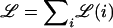. Here, the numerator is the likelihood of our observations given a disease hypothesis, and the denominator is the likelihood at random.

We will use P₀ to mean probability calculated according the random model and P_D to mean probability under the disease hypothesis. Thus, for example, we will write P(a|D,i) and P_D(a|i) interchangeably.

The disease affects the distribution of observed markers only by changing the probability distribution of ethnicity at the causal (disease) locus. Let a be the (hidden) number of A alleles for individual i at the causal locus. Thus, P_D(O|a,i)=P₀(O|a,i). We see that

and

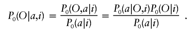Thus,

Equation (C1) is a key formula.

We see that P₀(a|O,i) is just the posterior distribution of our hidden state a in the HMM for individual i. Write P₀(a|O,i)=γ_t(a,i). Standard HMM calculations make the computation of γ_t(a,i) straightforward. P₀(a|i) is M_i(a), which we assume we know. Now, by standard conditional probability,

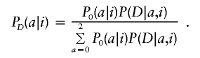We are, in effect, assuming that the conditional probability of disease depends only on ancestry at the causal locus. Thus, P(D|a,i) is independent of i. We will write P(D|a,i)=ψ(a). Therefore, P_D(a|i)∝M_i(a)ψ(a). This yields

Thus, we get

which simplifies to

Equation (C2) is the basic statistic used by our method. Our overall score at the locus under consideration is thus

as given the HMM parameters, the evidence for a disease locus is independent across individuals.

Note that, as it should be, the score ℒ(i) is invariant if we multiply ψ by a constant. Thus, we would obtain the same result by defining ψ(a)=P(D|a,i)/P(D). In fact, in our code and in the account given in the main article, we always normalize and take ψ(0)=1.

In practice, ψ is not likely to be known to us. Unless there is good evidence that the disease under study has a recessive component, we recommend the following multiplicative risk model: Take a range of r values, r₁,r₂,…,r_n, and, for the assumption r=r_i, set ψ(0)=1, ψ(1)=r, and ψ(2)=r². The procedure we have already described allows us to compute the Bayes factor F_i for the assumption r=r_i. We can now compute an overall Bayes factor F by

(This assumes a flat [uniform] prior on the assumptions r=r_i, which is all we have implemented, though this restriction could easily be relaxed.)

There is no need to restrict ourselves to r>1. A risk r<1 would imply a locus where ancestry in population A is protective.

Scoring with MCMC

The assumptions made in the previous section—that is, that we know various critical model parameters precisely—are unreasonable. As we discuss in the main article, seriously erroneous model parameters will mimic the effect of a true risk allele, so this is a problem that must be addressed. We use a large MCMC to solve our problem.

We have a large parameter space 𝒫. We think of 𝒫 as the space of parameters of the null model. Thus, in particular, the disease risk parameters ψ are not elements of 𝒫. Fix ψ for now. (We prefer to think of 𝒫 as the space of parameters outside the hidden HMM variables, which are the ancestry states of each individual at each locus. Therefore, 𝒫 includes all parameters necessary for the HMM we have already described but not the actual sequence of hidden states. )

Then, for any p∈𝒫, we can compute for each locus, using equations (C2) and (C3), the log Bayes factor ℒ. Here, ℒ=ℒ(p) depends on p, and we write

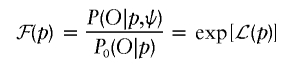for the Bayes factor, given p.

The following is a standard idea in Bayesian MCMC (see, e.g., Thompson and Guo [1991] or section 5.2.2 of Chen et al. [2000]). The Bayes factor ℱ at a locus is, by definition,

where Pr(p) is the prior distribution on our parameters. It is important to note that this prior is not dependent on our disease model and, in particular, is the same distribution in the causal and null case. Hence,

We can write this more compactly as 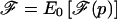, where E₀ is expectation under the posterior with the null hypothesis. Here we use the basic fact (Bayes’ theorem) that the null posterior distribution Post₀ satisfies Post₀(p)∝P₀(O|p)Pr(p). Equation (C2) has already shown how to efficiently compute ℒ(p)=logℱ(p).

So the Bayes factor we seek is just the expectation of the Bayes factor ℱ(p), with the expectation evaluated under the posterior distribution of p under the null model. MCMC techniques allow efficient sampling of 𝒫 under the posterior null model; further, the posterior state estimates γ_t(a,i), needed in equation (C2), are also computed under the null model. These two steps dominate the computational work. We then can efficiently estimate ℱ at each locus by computing the average of ℱ(p) after sampling with the MCMC. Note that the bulk of the work is independent of the assumed disease locus or risk model, an enormous computational savings.

Global Scoring and Significance

We recommend computing a genomewide score. For simplicity, assume that there is just one disease-related locus in the genome; then, it is natural to introduce a prior probability distribution, P(s), for the place in which a disease gene might be present. Then, our global score 𝒢 is just 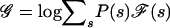, where ℱ(s) is the estimated Bayes factor for the hypothesis that the disease locus is s. As we discuss in our article, this is a powerful score, and we believe that it is the best statistic to use to test genomewide significance. Since 𝒢 is a Bayesian overall log factor, it allows direct calculation of the posterior degree of belief that there is genomic association with disease in the data being examined. We suggest in the main article that a log score (base 10) of 2 (LOD), corresponding to a Bayes factor of 100, should be regarded as showing significant evidence. Note that, as is common in Bayesian calculations, we are testing only one hypothesis here (a complex one involving many loci and possibly many risk models), and therefore no correction is needed for multiple hypotheses.

Finally, we remark that these scoring methods give an alternative methodology in linkage analysis and could be used instead of the Kruglyak-Lander thresholds (Lander and Kruglyak 1995) to test genomewide significance.

References

- Altshuler D, Hirschhorn JN, Klannemark M, Lindgren CM, Vohl MC, Nemesh J, Lane CR, Schaffner SF, Bolk S, Brewer C, Tuomi T, Gaudet D, Hudson TJ, Daly M, Groop L, Lander ES (2000) The common PPARγ Pro12Ala polymorphism is associated with decreased risk of type 2 diabetes. Nat Genet 26:76–80 10.1038/79216 [DOI] [PubMed] [Google Scholar]
- Balding DJ, Nichols RA (1995) A method for quantifying differentiation between populations at multi-allelic loci and its implications for investigating identity and paternity. Genetica 96:3–12 [DOI] [PubMed] [Google Scholar]
- Barcellos LF, Oksenberg JR, Begovich AB, Martin ER, Schmidt S, Vittinghoff E, Goodin DS, Pelletier D, Lincoln RR, Bucher P, Swerdlin A, Pericak-Vance MA, Haines JL, Hauser SL, Multiple Sclerosis Genetics Group (2003) HLA-DR2 dose effect on susceptibility to multiple sclerosis and influence on disease course. Am J Hum Genet 72:710–716 [DOI] [PMC free article] [PubMed] [Google Scholar]
- Baum LE, Petrie T, Soules G, Weiss N (1970) A maximization technique occurring in the statistical analysis of probabilistic functions of Markov chains. Ann Math Stat 41:164–171 [Google Scholar]
- Bickel PJ, Doksum KA (2001) Mathematical statistics: basic ideas and selected topics. Vol I. Second edition. Prentice Hall, New Jersey [Google Scholar]
- Botstein D, Risch N (2003) Discovering genotypes underlying human phenotypes: past successes for Mendelian disease, future approaches for complex disease. Nat Genet 33:228–237 10.1038/ng1090 [DOI] [PubMed] [Google Scholar]
- Briscoe D, Stephens JC, O’Brien SJ (1994) Linkage disequilibrium in admixed populations: Applications in gene mapping. J Hered 85:59–63 [PubMed] [Google Scholar]
- Carlson CS, Eberle MA, Rieder MJ, Smith JD, Kruglyak L, Nickerson DA (2003) Additional SNPs and linkage-disequilibrium analyses are necessary for whole-genome association studies in humans. Nat Genet 33:518–521 10.1038/ng1128 [DOI] [PubMed] [Google Scholar]
- Chakraborty R, Weiss KM (1988) Admixture as a tool for finding linked genes and detecting that difference from allelic association between loci. Proc Natl Acad Sci USA 85:9119–9123 [DOI] [PMC free article] [PubMed] [Google Scholar]
- Chen M-H, Shao Q-M, Ibrahim JG (2000) Monte Carlo methods in Bayesian computation. Springer, New York [Google Scholar]
- Collins FS, Guyer MS, Charkravarti A (1997) Variations on a theme: cataloging human DNA sequence variation. Science 278:1580–1581 10.1126/science.278.5343.1580 [DOI] [PubMed] [Google Scholar]
- Collins-Schramm HE, Chima B, Operario DJ, Criswell LA, Seldin MF (2003) Markers informative for ancestry demonstrate consistent megabase-length linkage disequilibrium in the African American population. Hum Genet 113:211–219 10.1007/s00439-003-0961-1 [DOI] [PubMed] [Google Scholar]
- Corbo RM, Scacchi R (1999) Apolipoprotein E (APOE) allele distribution in the world. Is APOE*4 a “thrifty” allele? Ann Hum Genet 63:301–310 10.1046/j.1469-1809.1999.6340301.x [DOI] [PubMed] [Google Scholar]
- Crocq MA, Buguet A, Bisser S, Burgert E, Stanghellini A, Uyanik G, Dumas M, Macher JP, Mayerova A (1996) BalI and MspI polymorphisms of the dopamine D3 receptor gene in African Blacks and Caucasians. Hum Hered 46:58–60 [DOI] [PubMed] [Google Scholar]
- Daly MJ, Rioux JD, Schaffner SF, Hudson TJ, Lander ES (2001) High-resolution haplotype structure in the human genome. Nat Genet 29:229–232 10.1038/ng1001-229 [DOI] [PubMed] [Google Scholar]
- Davey Smith G, Neaton JD, Wentworth D, Stamler R, Stamler J (1998) Mortality differences between black and white men in the USA: contribution of income and other risk factors among men screened for the MRFIT. MRFIT Research Group. Multiple Risk Factor Intervention Trial. Lancet 351:934–939 10.1016/S0140-6736(00)80010-0 [DOI] [PubMed] [Google Scholar]
- Devlin B, Roeder K (1999) Genomic control for association studies. Biometrics 55:997–1004 [DOI] [PubMed] [Google Scholar]
- Donner H, Rau H, Walfish PG, Braun J, Siegmund T, Finke R, Herwig J, Usadel KH, Badenhoop K (1997) CTLA4 alanine-17 confers genetic susceptibility to Graves’ disease and to type 1 diabetes mellitus. J Clin Endocrinol Metab 82:143–146 10.1210/jc.82.1.143 [DOI] [PubMed] [Google Scholar]
- Durbin R, Eddy S, Krogh A, Mitchison G (1998) Biological sequence analysis. Cambridge University Press, Cambridge [Google Scholar]
- Falush D, Stephens M, Pritchard JK (2003) Inference of population structure using multilocus genotype data: linked loci and correlated allele frequencies. Genetics 164:1567–1587 [DOI] [PMC free article] [PubMed] [Google Scholar]
- Farrer LA, Cupples LA, Haines JL, Hyman B, Kukull WA, Mayeux R, Myers RH, Pericak-Vance MA, Risch N, van Duijn CM (1997) Effects of age, sex, and ethnicity on the association between apolipoprotein E genotype and Alzheimer disease: a meta-analysis. APOE and Alzheimer Disease Meta Analysis Consortium. JAMA 278:1349–1356 [PubMed] [Google Scholar]
- Gabriel SB, Schaffner SF, Nguyen H, Moore JM, Roy J, Blumenstiel B, Higgins J, DeFelice M, Lochner A, Faggart M, Liu-Cordero SN, Rotimi C, Adeyemo A, Cooper R, Ward R, Lander ES, Daly MJ, Altshuler D (2002) The structure of haplotype blocks in the human genome. Science 296:2225–2229 10.1126/science.1069424 [DOI] [PubMed] [Google Scholar]
- Gelman A, Carlin JB, Stern HS, Rubin DB (1995) Bayesian data analysis. Chapman and Hall, London [Google Scholar]
- Giallourakis C, Stoll M, Miller K, Hampe J, Lander ES, Daly MJ, Schreiber S, Rioux JD (2003) IBD5 is a general risk factor for inflammatory bowel disease: replication of association with Crohn disease and identification of a novel association with ulcerative colitis. Am J Hum Genet 73:205–211 [DOI] [PMC free article] [PubMed] [Google Scholar]
- Gilks WR, Best NG, Tan KKC (1995) Adaptive rejection Metropolis sampling within Gibbs sampling. Appl Stat 44:455–472 [Google Scholar]
- Gilks WR, Richardson S, Spiegelhalter DJ (Eds) (1996) Markov Chain Monte Carlo in practice. Chapman and Hall, London [Google Scholar]
- Gilks WR, Wild P (1992) Adaptive rejection sampling for Gibbs sampling. Appl Stat 41:337–348 [Google Scholar]
- Halder I, Shriver MD (2003) Measuring and using admixture to study the genetics of complex disease. Hum Genom 1:52–62 [DOI] [PMC free article] [PubMed] [Google Scholar]
- Hill AV, Allsopp CE, Kwiatkowski D, Anstey NM, Twumasi P, Rowe PA, Bennett S, Brewster D, McMichael AJ, Greenwood BM (1991) Common west African HLA antigens are associated with protection from severe malaria. Nature 352:595–600 10.1038/352595a0 [DOI] [PubMed] [Google Scholar]
- Hirschhorn JN, Lohmueller K, Byrne E, Hirschhorn K (2002) A comprehensive review of genetic association studies. Genet Med 4:45–61 10.1097/00125817-200203000-00002 [DOI] [PubMed] [Google Scholar]
- Hoggart CJ, Parra EJ, Shriver MD, Bonilla C, Kittles RA, Clayton DG, McKeigue PM (2003) Control of confounding of genetic associations in stratified populations. Am J Hum Genet 72:1492–1504 [DOI] [PMC free article] [PubMed] [Google Scholar]
- Kurtzke JF, Beebe GW, Norman JE Jr (1979) Epidemiology of multiple sclerosis in US veterans. 1. Race, sex, and geographic distribution. Neurology 29:1228–1235 [DOI] [PubMed] [Google Scholar]
- Lander ES, Green P (1987) Construction of multilocus genetic linkage maps in humans. Proc Natl Acad Sci USA 84:2363–2367 [DOI] [PMC free article] [PubMed] [Google Scholar]
- Lander E, Kruglyak L (1995) Genetic dissection of complex traits: guidelines for interpreting and reporting linkage results. Nat Genet 11:241–247 [DOI] [PubMed] [Google Scholar]
- Lautenberger JA, Stephens JC, O’Brien SJ, Smith M (2000) Significant admixture linkage disequilibrium across 30 cM around the FY locus in African-Americans. Am J Hum Genet 66:969–978 [DOI] [PMC free article] [PubMed] [Google Scholar]
- Lockwood JR, Roeder K, Devlin B (2001) A Bayesian hierarchical model for allele frequencies. Genet Epidemiol 20:17–33 10.1002/1098-2272(200101)20:1<17::AID-GEPI3>3.0.CO;2-Q [DOI] [PubMed] [Google Scholar]
- Lohmueller KE, Pearce CL, Pike M, Lander ES, Hirschhorn JN (2003) Meta-analysis of genetic association studies supports a contribution of common variants to susceptibility to common disease. Nat Genet 33:177–182 10.1038/ng1071 [DOI] [PubMed] [Google Scholar]
- McKeigue PM (1997) Mapping genes underlying ethnic differences in disease risk by linkage disequilibrium in recently admixed populations. Am J Hum Genet 60:188–196 [PMC free article] [PubMed] [Google Scholar]
- ——— (1998) Mapping genes that underlie ethnic differences in disease risk: methods for detecting linkage in populations, by conditioning on parental admixture. Am J Hum Genet 63:241–251 [DOI] [PMC free article] [PubMed] [Google Scholar]
- McKeigue PM, Carpenter JR, Parra EJ, Shriver MD (2000) Estimation of admixture and detection of linkage in admixed populations by a Bayesian approach: application to African-American populations. Ann Hum Genet 64:171–186 10.1046/j.1469-1809.2000.6420171.x [DOI] [PubMed] [Google Scholar]
- Mead S, Mahal SP, Beck J, Campbell T, Farrall M, Fisher E, Collinge (2001) Sporadic—but not variant—Creutzfeldt-Jakob disease is associated with polymorphisms upstream of PRNP exon 1. Am J Hum Genet 69:1225–1235 [DOI] [PMC free article] [PubMed] [Google Scholar]
- Nakajima T, Jorde LB, Ishigami T, Umemura S, Emi M, Lalouel JM, Inoue I (2002) Nucleotide diversity and haplotype structure of the human angiotensinogen gene in two populations. Am J Hum Genet 70:108–123 [DOI] [PMC free article] [PubMed] [Google Scholar]
- Nicholson G, Smith A, Jónsson F, Gústafson Ó, K S, Donnelley P (2002) Assessing population differentiation and isolation from single-nucleotide polymorphism data. J Roy Stat Soc Ser B 64:695–715 10.1111/1467-9868.00357 [DOI] [Google Scholar]
- Oksenberg JR, Barcellos LF, Cree BA, Baranzini SE, Bugawan TL, Khan O, Lincoln RR, Swerdlin A, Mignot E, Lin L, Goodin D, Erlich HA, Schmidt S, Thomson G, Reich DE, Pericak-Vance MA, Haines JL, Hauser SL (2004) Mapping multiple sclerosis susceptibility to the HLA-DR locus in African Americans. Am J Hum Genet 74:160–167 [DOI] [PMC free article] [PubMed] [Google Scholar]
- Osei-Hyiaman D, Hou L, Zhiyin R, Zhiming Z, Yu H, Amankwah AA, Harada S (2001) Association of a novel point mutation (C159G) of the CTLA4 gene with type 1 diabetes in West Africans but not in Chinese. Diabetes 50:2169–2171 [DOI] [PubMed] [Google Scholar]
- Parra EJ, Marcini A, Akey J, Martinson J, Batzer MA, Cooper R, Forrester T, Allison DB, Deka R, Ferrell RE, Shriver MD (1998) Estimating African-American admixture proportions by use of population-specific alleles. Am J Hum Genet 63:1839–1851 [DOI] [PMC free article] [PubMed] [Google Scholar]
- Permutt MA, Elbein SC (1990) Insulin gene in diabetes. Analysis through RFLP. Diabetes Care 13:364–374 [DOI] [PubMed] [Google Scholar]
- Pfaff CL, Parra EJ, Bonilla C, Hiester K, McKeigue PM, Kamboh MI, Hutchinson RG, Ferrell RE, Boerwinkle E, Shriver MD (2001) Population structure in admixed populations: effect of admixture dynamics on the pattern of linkage disequilibrium. Am J Hum Genet 68:198–207 [DOI] [PMC free article] [PubMed] [Google Scholar]
- Rabiner LR (1989) A tutorial on hidden Markov models. Proceedings of the IEEE 77:257–286 10.1109/5.18626 [DOI] [Google Scholar]
- Rees DC, Cox M, Clegg JB (1995) World distribution of factor V Leiden. Lancet 346:1133–1134 10.1016/S0140-6736(95)91803-5 [DOI] [PubMed] [Google Scholar]
- Ripley BD (1987) Stochastic simulation. Wiley, New York [Google Scholar]
- Rioux JD, Daly MJ, Silverberg MS, Lindblad K, Steinhart H, Cohen Z, Delmonte T, et al (2001) Genetic variation in the 5q31 cytokine gene cluster confers susceptibility to Crohn disease. Nat Genet 29:223–228 10.1038/ng1001-223 [DOI] [PubMed] [Google Scholar]
- Risch N (1992) Mapping genes for complex disease using association studies with recently admixed populations. Am J Hum Genet Suppl 51:13 [Google Scholar]
- Risch N, Merikangas K (1996) The future of genetic studies of complex human diseases. Science 273:1516–1517 [DOI] [PubMed] [Google Scholar]
- Risch NJ (2000) Searching for genetic determinants in the new millennium. Nature 405:847–856 10.1038/35015718 [DOI] [PubMed] [Google Scholar]
- Rosendaal FR, Koster T, Vandenbroucke JP, Reitsma PH (1995) High risk of thrombosis in patients homozygous for factor V Leiden (activated protein C resistance). Blood 85:1504–1508 [PubMed] [Google Scholar]
- Rotimi C, Puras A, Cooper R, McFarlane-Anderson N, Forrester T, Ogunbiyi O, Morrison L, Ward R (1996) Polymorphisms of renin-angiotensin genes among Nigerians, Jamaicans, and African Americans. Hypertension 27:558–563 [DOI] [PubMed] [Google Scholar]
- Shriver MD, Parra EJ, Dios S, Bonilla C, Norton H, Jovel C, Pfaff C, Jones C, Massac A, Cameron N, Baron A, Jackson T, Argyropoulos G, Jin L, Hoggart CJ, McKeigue PM, Kittles RA (2003) Skin pigmentation, biogeographical ancestry and admixture mapping. Hum Genet 112:387–399 [DOI] [PubMed] [Google Scholar]
- Siddiqui A, Kerb R, Weale ME, Brinkmann U, Smith A, Goldstein DB, Wood NW, Sisodiya SM (2003) Association of multidrug resistance in epilepsy with a polymorphism in the drug-transporter gene ABCB1. N Engl J Med 348:1442–1448 10.1056/NEJMoa021986 [DOI] [PubMed] [Google Scholar]
- Siffert W, Forster P, Jockel KH, Mvere DA, Brinkmann B, Naber C, Crookes R, et al (1999) Worldwide ethnic distribution of the G protein β3 subunit 825T allele and its association with obesity in Caucasian, Chinese, and Black African individuals. J Am Soc Nephrol 10:1921–1930 [DOI] [PubMed] [Google Scholar]
- Smith MW, Lautenberger JA, Shin HD, Chretien JP, Shrestha S, Gilbert DA, O’Brien SJ (2001) Markers for mapping by admixture linkage disequilibrium in African American and Hispanic populations. Am J Hum Genet 69:1080–1094 [DOI] [PMC free article] [PubMed] [Google Scholar]
- Smith MW, Patterson N, Lautenberger JA, Truelove AL, McDonald GJ, Waliszewska A, Kessing BD, et al (2004) A high-density admixture map for disease gene discovery in African Americans. Am J Hum Genet 74:1001–1013 (in this issue) [DOI] [PMC free article] [PubMed] [Google Scholar]
- Soldevila M, Calafell F, Andres AM, Yague J, Helgason A, Stefansson K, Bertranpetit J (2003) Prion susceptibility and protective alleles exhibit marked geographic differences. Hum Mutat 22:104–105 10.1002/humu.9157 [DOI] [PubMed] [Google Scholar]
- Stephens JC, Briscoe D, O’Brien SJ (1994) Mapping by admixture linkage disequilibrium in human populations: limits and guidelines. Am J Hum Genet 55:809–824 [PMC free article] [PubMed] [Google Scholar]
- Thompson EA, Guo SW (1991) Evaluation of likelihood ratios for complex genetic models. J Math Appl Med Biol 8:149–169 [DOI] [PubMed] [Google Scholar]
- Ueda H, Howson JM, Esposito L, Heward J, Snook H, Chamberlain G, Rainbow DB, et al (2003) Association of the T-cell regulatory gene CTLA4 with susceptibility to autoimmune disease. Nature 423:506–511 10.1038/nature01621 [DOI] [PubMed] [Google Scholar]
- Wallin MT, Page WF, Kurtzke JF (2003) Multiple sclerosis in US veterans of the Vietnam era and later military service: race, sex, and geography. Ann Neurol 55:65–71 10.1002/ana.10788 [DOI] [PubMed] [Google Scholar]
- Wilson JF, Goldstein DB (2000) Consistent long-range linkage disequilibrium generated by admixture in a Bantu-Semitic hybrid population. Am J Hum Genet 67:926–935 [DOI] [PMC free article] [PubMed] [Google Scholar]
- Zheng C, Elston RC (1999) Multipoint linkage disequilibrium mapping with particular reference to the African-American population. Genet Epidemiol 17:79–101 10.1002/(SICI)1098-2272(1999)17:2<79::AID-GEPI1>3.0.CO;2-N [DOI] [PubMed] [Google Scholar]