Bias toward the Null Hypothesis in Model-Free Linkage Analysis Is Highly Dependent on the Test Statistic Used

Abstract

Recently, it has been suggested that traditional nonparametric multipoint-linkage procedures can show a “bias” toward the null hypothesis of no effect when there is incomplete information about allele sharing at genotyped marker loci (or at positions in between marker loci). Here, I investigate the extent of this bias for a variety of test statistics commonly used in qualitative- (“affecteds only”) and quantitative-trait linkage analysis. Through simulation and analytical derivation, I show that many of the test statistics available in standard linkage analysis packages (such as Genehunter, Merlin, and Allegro) are, in fact, not affected by this bias problem. A few test statistics—most notably the nonparametric linkage statistic and, to a lesser extent, the Aspex-MLS and Haseman-Elston statistics—are affected by the bias. Variance-components procedures, although unbiased, can show inflation or deflation of the test statistic attributable to the inclusion of pairs with incomplete identity-by-descent information. Results obtained—for instance, in genome scans—using these methods might therefore be worth revisiting to see if greater power can be obtained by use of an alternative statistic or by eliminating or downweighting uninformative relative pairs.

In a recent article, Schork and Greenwood (2004) demonstrated a “bias” that can occur in nonparametric (model-free) linkage analysis when relative pairs whose identity-by-descent (IBD) allele sharing is uncertain are kept in the analysis and are assigned expected values for IBD sharing. Since these expected values are calculated under the null hypothesis of no linkage, this results in a “dilution” of the data set, with regard to the evidence for linkage that it provides, and a consequent “dragging down” of the linkage test statistic. Schork and Greenwood (2004) recommend one easy solution: simply remove uninformative relative pairs from the analysis; however, they point out that, in practice, it can be difficult to decide which relative pairs to remove if the pairs are not completely uninformative, since one would have to make a potentially arbitrary decision about what level of informativity to use as a cutoff for a pair to be included/excluded. Other solutions recommended are to increase the overall informativity by use of a denser genetic map or to consider the use of more complicated test procedures (such as procedures that downweight uninformative relative pairs in some way) or by use of appropriate mixture models. In light of their findings, Schork and Greenwood (2004) recommend that researchers who have conducted linkage studies in the past and who ignored or were not aware of the bias problem should perhaps revisit their analyses.

Although the conclusions of Schork and Greenwood (2004) might seem disturbing, their conclusions result, in part, from consideration of the particular test statistic that they chose to investigate. Schork and Greenwood (2004) defined a likelihood-ratio test statistic—or LOD score—based on a multinomial distribution for IBD sharing, and they demonstrated that “adding in” expected IBD observations from pairs that are, in fact, uninformative will dilute this test statistic toward the null. However, the test statistic Schork and Greenwood (2004) considered does not, in fact, precisely correspond to the test statistics available in many standard genetic linkage analysis packages, such as Genehunter (Kruglyak and Lander 1995; Kruglyak et al. 1996), Allegro (Gudbjartsson et al. 2000), Merlin (Abecasis et al. 2002), or Aspex. These packages already calculate test statistics that make some allowance for uncertainty in IBD sharing. Therefore, it is of interest to examine whether use of these more complicated (but nevertheless fairly standard) test statistics correct the bias problem noted by Schork and Greenwood (2004).

A variety of test statistics have been proposed for performing nonparametric (model-free) linkage analysis with affected sib pairs. Here, I will concentrate on those that are best known and available in the standard packages mentioned above.

A likelihood-ratio test statistic for linkage in affected sib pairs can be derived as follows (Risch 1990a, 1990b, 1990c; Holmans 1993). Let M denote the observed marker genotype data for a family consisting of two siblings plus parents, let A denote the event that both siblings are affected with some disease of interest, and let IBD=i denote the event that the siblings share i alleles IBD at some position in the genome. Then the likelihood contribution for the jth sib pair, conditional on the ascertainment scheme (i.e., on the fact that both sibs are affected), is

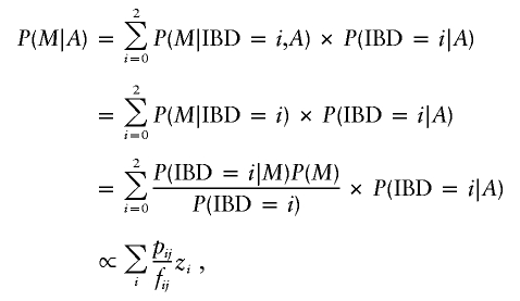where z_i is a vector of parameters representing the probabilities that an affected sib pair shares i=0, 1, or 2 alleles IBD, f_ij is the prior probability (given relationship only), and p_ij the posterior probability (given relationship and observed marker data) that sib pair j shares i alleles IBD. For a sib pair, these prior probabilities are just f_0j=0.25, f_1j=0.5, f_2j=0.25, and the posterior probabilities may be calculated, given the observed marker data, using programs such as Genehunter, Allegro, or Merlin.

An overall maximum LOD score (MLS) test statistic may be defined as

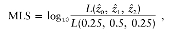where represent the maximum-likelihood estimates of the sharing parameters, and the likelihood (for the entire sample of sib pairs) may be written as

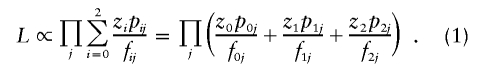Note that, for completely informative data (i.e., when the IBD sharing is known with certainty), this MLS statistic is identical to the statistic considered by Schork and Greenwood (2004). However, the statistics differ with regard to the treatment of uninformative pairs. If a pair is completely uninformative, so that the posterior probabilities are p_0j=0.25, p_1j=0.5, and p_2j=0.25, then, in the MLS statistic, the posterior and prior probabilities cancel out, and the likelihood contribution for the pair is , giving a log-likelihood contribution of 0, so that the pair makes no contribution to the resulting likelihood-ratio test statistic. For the MLS statistic, therefore, it should make absolutely no difference whether the pair is included in the calculation.

The MLS statistic defined above may be calculated in Genehunter with the “estimate” command. Genehunter uses a restricted maximization, proposed by Holmans (1993), that restricts the values of the sharing parameters to values that lie in a possible triangle consistent with genetic segregation. Genehunter can additionally calculate an MLS that is further restricted to correspond to a situation of “no dominance variance,” which essentially restricts the value of to equal 0.5. An MLS with an unrestricted maximization may be calculated in the program Aspex. Aspex and Genehunter differ slightly in the way that the multipoint posterior probabilities p_ij are calculated, and this will be seen below (in the simulation study) to have some importance with regard to the performance of the two programs in the presence of uninformative pairs.

Another popular statistic for model-free linkage analysis is the nonparametric linkage (NPL) statistic, available in such programs as Genehunter, Allegro, and Merlin. This statistic is based on scoring functions proposed by Whittemore and Halpern (1994). For a sample consisting solely of affected sib pairs (as opposed to also including other types of affected relative pairs), the NPL statistic is equivalent to a test of the mean proportion of alleles shared IBD (the “mean test”) proposed by Blackwelder and Elston (1985). Suppose that, for pedigree i, we have complete information, in the sense that we know the inheritance vector ν_i at a given location on the genome. Then, we define a score, S_i, that is based on the number of alleles shared IBD by the affected members of the pedigree, and a normalized score,

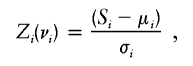where μ_i and σ_i are the mean and SD of S_i, respectively, under the null hypothesis of no linkage, calculated by enumeration of all possible inheritance vectors (which, under null hypothesis, are all equally likely), regardless of whether they are compatible with observed genotype data. For incomplete data, we instead use a score , which is the expected value of S_i evaluated over all inheritance vectors compatible with observed genotype data (in the correct proportion, given the observed data), and a normalized score,

An overall test statistic can be constructed as a weighted average of the test statistics from the different pedigrees. Note that, here, we approximate the null SD of by σ_i, the null SD of S_i. This is known as the “perfect data approximation” and results in a conservative test (Kruglyak et al. 1996; Kong and Cox 1997) when the IBD sharing is not known with certainty. Because the score is the expected value of S_i evaluated over the possible underlying inheritance vectors (i.e., evaluated over the possible IBD-sharing configurations), a relative pair for which IBD sharing is uncertain will still contribute to the test statistic. The exact contribution depends on the scoring function used; under one popular scheme (“pairs” scoring), a sib pair with posterior IBD-sharing probabilities p_0j=0.25, p_1j=0.5, and p_2j=0.25 will contribute exactly the same score as if the pair had been observed to share exactly 1 allele IBD. It would therefore seem likely that this NPL test statistic could be affected by the bias problem suggested by Schork and Greenwood (2004).

In practice, the bias potentially incurred when using the NPL test statistic can be avoided by use of two alternative statistics, denoted here as “Z-lin” and “Z-exp,” which are based on normalized likelihood-ratio (Z_lr) statistics. These statistics were originally proposed by Kong and Cox (1997) to avoid the power loss caused by the “perfect data approximation” in the NPL approach. Kong and Cox (1997) construct a likelihood on the basis of either a linear or exponential model, parameterized by a parameter δ that represents the magnitude of deviation from null IBD sharing, and they note that the score test from the linear or exponential likelihood is equivalent to the previously proposed NPL method. However, Kong and Cox (1997) propose testing the null hypotheses that δ=0 with a likelihood-ratio test that is based on an exact log likelihood, even in the presence of missing data and thus uncertain IBD information. The Z_lr test statistic is defined as

where denotes the log-likelihood ratio; for example, for the exponential model,

and c_i(δ)^-1 is a normalization constant satisfying

Given a sib pair with posterior IBD-sharing probabilities p_0j=0.25, p_1j=0.5, and p_2j=0.25, the contribution E_H0[exp(δZ_i)|markerdata] can be shown to equal the normalization constant c_i(δ)^-1, and so the contribution to the log likelihood from this sib pair will again be 0. For the Z_lr statistics, therefore, one would again not expect it to make any difference whether the pair is included in the calculation. Provided a genome screen has been performed using Z_lr statistics (available in programs such as Allegro, Merlin, and Genehunter-Plus) rather than with NPL statistics, the bias problem is therefore unlikely to be an issue. As an alternative, one could use NPL statistics and derive correct P values by use of simulations, although, for genome screens, such approaches may be prohibitively time consuming.

To demonstrate the performance of the different test statistics in practice, I performed a simulation study. I simulated replicates of 200 affected sib pairs by use of the same six underlying genetic models considered by Schork and Greenwood (2004). Initially, I used a single genetic marker located at the disease locus, and I attempted to analyze replicates in which varying proportions of the 200 sib pairs were assumed to be completely uninformative (genotypes missing or parents homozygous), with the remaining pairs all completely informative. However, it proved impossible to compare the performance of the methods when applied to the full data set (with the uninformative pairs kept in the analysis) compared with when the uninformative pairs were excluded from the analysis, because every linkage analysis package that I tried recognized the pairs that were uninformative and automatically discarded them from the analysis! (However, it was possible to output posterior IBD-sharing probabilities for these pairs, if desired.) It was encouraging to see that most linkage analysis packages were able to automatically detect and discard such pairs, but, in practice, of course, the problem would arise with pairs that show low informativity in certain chromosomal regions rather than with pairs that are entirely uninformative. To assess the performance of the statistics, I therefore simulated a more-complex scenario involving three linked markers positioned 100 cM apart, with the central marker located at the disease locus. The informative pairs had complete IBD information at each of the three markers, whereas the uninformative pairs had complete information at the two outer (flanking) markers but no information at the inner (disease) locus. By use of multipoint methods, these essentially uninformative pairs could be included in the analysis because of the very small amount of information coming from the linked flanking markers.

Table 1 shows the average difference between the test statistic calculated at the disease locus position, with uninformative pairs removed from the analysis and the one calculated with the uninformative pairs kept in the analysis (means and SDs of the difference over 100 replicates). Results are shown for six test statistics calculated using the linkage packages Genehunter, Allegro, and Aspex; results for the NPL statistic were virtually identical among the packages Genehunter, Allegro, and Merlin, and results for the Z-lin statistic were virtually identical between the packages Allegro and Merlin (data not shown). For every simulation model considered, it can be seen that the MLS statistics from Genehunter (MLS-gh and MLS-ndv) and the Z_lr statistics from Allegro (Z-lin and Z-exp) are not affected by the bias problem described by Schork and Greenwood (2004); it makes no difference whether the uninformative pairs are removed from the analysis—on average, there is no difference between the test statistics. For the NPL statistic (calculated in either Genehunter, Allegro, or Merlin), however, the bias problem is quite apparent. In some simulation scenarios, even a small percentage of uninformative pairs causes the NPL statistic to be considerably reduced when the uninformative pairs are retained in the analysis, resulting in the positive difference between the statistics shown in table 1. With 50% uninformative pairs, the effect is quite pronounced; for example, in simulation scenario 5, the NPL is reduced by 1.86, on average, when the pairs are retained compared with when they are discarded. It is interesting that the MLS statistic calculated using the “sib_phase” option in Aspex (MLS-aspex) also suffers to a lesser extent from the bias problem, suggesting that, in the Aspex package, the calculation of this statistic in the presence of incomplete IBD information differs from the calculation as described here (eq. [1]) and performed by Genehunter.

Table 1.

Results from Simulations Performed to Assess Impact of Uninformative Sibling Pairs on Linkage Analysis for Different Test Statistics^[Note]

	Difference between Test Statisticsb by % Uninformative
	5%		10%		25%		50%
Simulationand TestStatistica	Mean	SE	Mean	SE	Mean	SE	Mean	SE
1:
NPL	.1699	.0488	.3461	.0815	.8379	.1400	1.4854	.2458
Z-lin	.0004	.0052	−.0006	.0076	−.0006	.0135	−.0004	.0241
Z-exp	.0004	.0054	−.0006	.0079	−.0008	.0141	−.0007	.0251
MLS-gh	.0012	.0170	−.0018	.0244	−.0028	.0396	−.0024	.0591
MLS-ndv	.0012	.0165	−.0018	.0236	−.0023	.0380	−.0019	.0566
MLS-aspex	.0395	.1582	.0412	.2232	.1219	.3589	.2583	.5198
2:
NPL	.1084	.0449	.2176	.0718	.5214	.1312	.9361	.2618
Z-lin	.0004	.0061	.0000	.0087	.0025	.0163	.0001	.0284
Z-exp	.0003	.0061	.0000	.0087	.0025	.0165	−.0003	.0286
MLS-gh	.0008	.0117	.0003	.0165	.0051	.0303	.0010	.0431
MLS-ndv	.0008	.0114	.0003	.0162	.0049	.0292	.0010	.0431
MLS-aspex	.0189	.1054	.0268	.1496	.1003	.2762	.1182	.3809
3:
NPL	.1323	.0491	.2641	.0754	.6309	.1418	1.0807	.2613
Z-lin	.0002	.0069	−.0005	.0094	−.0022	.0152	−.0038	.0267
Z-exp	.0002	.0070	−.0005	.0096	−.0023	.0155	−.0039	.0272
MLS-gh	.0009	.0159	−.0008	.0224	−.0039	.0319	−.0059	.0469
MLS-ndv	.0009	.0154	−.0007	.0216	−.0036	.0307	−.0056	.0448
MLS-aspex	.0250	.1450	.0267	.2032	.0479	.2918	.0962	.4135
4:
NPL	.0073	.0236	.0141	.0442	.0489	.1180	.0947	.2176
Z-lin	−.0005	.0039	−.0016	.0069	−.0009	.0138	−.0018	.0195
Z-exp	−.0006	.0052	−.0014	.0083	−.0008	.0156	−.0007	.0265
MLS-gh	−.0002	.0024	−.0003	.0031	−.0003	.0056	−.0006	.0094
MLS-ndv	−.0003	.0023	−.0003	.0029	−.0003	.0052	−.0009	.0085
MLS-aspex	−.0025	.0220	−.0028	.0330	.0007	.0541	−.0050	.0870
5:
NPL	.2288	.0741	.4364	.0953	1.0399	.1568	1.8594	.2205
Z-lin	−.0003	.0055	−.0006	.0080	.0000	.0151	.0026	.0242
Z-exp	−.0003	.0060	−.0006	.0087	.0001	.0163	.0027	.0262
MLS-gh	−.0011	.0241	−.0025	.0342	.0002	.0580	.0079	.0767
MLS-ndv	−.0011	.0233	−.0024	.0327	.0002	.0565	.0074	.0743
MLS-aspex	.0414	.2305	.0737	.3223	.2442	.5281	.5341	.6792
6:
NPL	.1128	.0400	.2175	.0632	.5218	.1386	.9335	.2714
Z-lin	−.0008	.0061	−.0017	.0091	−.0021	.0149	−.0016	.0266
Z-exp	−.0008	.0062	−.0017	.0092	−.0021	.0151	−.0015	.0268
MLS-gh	−.0018	.0124	−.0039	.0190	−.0029	.0281	−.0006	.0411
MLS-ndv	−.0018	.0121	−.0038	.0183	−.0028	.0270	−.0008	.0398
MLS-aspex	−.0060	.1113	−.0121	.1701	.0324	.2543	.1104	.3713

Note.— Means and SEs of test statistic are given over 100 replicates.

^aTest statistics considered were as follows: NPL = NPL statistic calculated using Allegro; Z-lin = allele-sharing statistic Z_lr calculated under linear model, by use of Allegro; Z-exp = allele-sharing statistic Z_lr calculated under exponential model, by use of Allegro; MLS-gh = MLS statistic (“loglike”) calculated using estimate command in Genehunter; MLS-ndv = MLS statistic (“loglike”) calculated using estimate command, with no dominance variance in Genehunter; and MLS-aspex = MLS statistic on 2 df, calculated using ASPEX.

^bThe difference between the test statistic achieved when uninformative pairs are removed from the analysis and that achieved when they are kept in the analysis

For a statistician, the concept of “bias” usually applies to parameter estimates rather than to test statistics; in particular, it refers to whether the expected value of a parameter estimate obtained from some analysis procedure is equal to its true value. For affected-sib-pair studies, a natural parameterization is in terms of the IBD-sharing probabilities , conditional on the fact that a pair is affected. These sharing probabilities are functions of the underlying genetic parameters (disease penetrances and disease-allele frequencies) but, unlike the underlying genetic parameters, may be estimated from affected-sib-pair data. Note that the probabilities are not the same as the average (over pairs; i.e., over j) of the posterior probabilities p_ij, since the posterior probabilities p_ij are calculated conditional on the marker data but not conditional on the fact that the pair is affected. The appropriate way to estimate is not, therefore, to output and average the posterior probabilities p_ij but, rather, to use maximum-likelihood estimation of the likelihood in equation (1). The only methods considered in the simulation study that produce maximum-likelihood estimates of are the MLS methods implemented in Genehunter and Aspex. (The Z_lr methods implemented in Allegro and Merlin produce estimates of a different sharing parameter, δ; however, the relationship between δ and the underlying genetic parameters is unclear.)

Table 2 shows the mean (over 100 simulation replicates) of the parameter estimates as obtained using the programs Genehunter (MLS-gh) and Aspex (MLS-aspex), with a sample size of either 200 or 1,000 affected sib pairs and 50% of the sample deemed uninformative (but retained in the analysis). Even in this extreme situation with regard to informativity, the parameter estimates are seen to be essentially unbiased. The estimates from Genehunter differ slightly from the true values (i.e., show a very slight bias), as expected from the fact that Genehunter employs a restricted maximization under “possible triangle constraints” (Holmans 1993). This means that maximum-likelihood estimates that fall outside the possible triangle of plausible genetic values are adjusted to move into the possible triangle, resulting in a slight bias in this case away from (rather than toward) the null hypothesis. This effect will disappear asymptotically, as demonstrated by the closer correspondence between the estimates and the true values with the larger sample size of 1,000. The Aspex analysis uses an unrestricted maximization (by use of the “sib_phase” option with a 2-df test) and shows no discernible bias for either sample size.

Table 2.

Parameter Estimates for Sharing Parameters (z₀, z₁, z₂) under Different Simulation Models, When 50% of Samples Are Uninformative^[Note]

	True			MLS-gh			MLS-aspex
Sample Size and Simulation	z0	z1	z2	z0	z1	z2	z0	z1	z2
200:
1	.077	.500	.423	.076	.477	.447	.073	.492	.434
2	.142	.500	.358	.139	.486	.375	.135	.505	.361
3	.119	.500	.381	.127	.477	.397	.122	.493	.384
4	.243	.498	.260	.234	.491	.275	.235	.507	.258
5	.026	.500	.474	.026	.482	.492	.025	.500	.474
6	.144	.500	.356	.144	.479	.377	.139	.496	.365
1,000:
1	.077	.500	.423	.078	.491	.431	.076	.500	.423
2	.142	.500	.358	.142	.493	.365	.140	.501	.359
3	.119	.500	.381	.124	.491	.384	.122	.501	.377
4	.243	.498	.260	.240	.494	.266	.243	.496	.261
5	.026	.500	.474	.027	.489	.484	.026	.497	.476
6	.144	.500	.356	.145	.489	.367	.142	.496	.361

Note.— Mean values of the sharing parameters are given over 100 replicates.

It seems, therefore, as if many of the most popular methods for affected-relative-pair analysis are not affected by the bias problem noted by Schork and Greenwood (2004). A final question of interest is whether nonparametric methods for linkage analysis of quantitative traits may be affected by the bias. Two widely used methods for linkage analysis of quantitative traits are the Haseman-Elston (H-E) method (Haseman and Elston 1972) and the variance-components (VC) method (Amos 1994; Almasy and Blangero 1998). More recent versions of these methods have included the H-E “revisited” method (Elston et al. 2000), the “unified” H-E method (Xu et al. 2000), and an alternative regression-based approach (Sham et al. 2002). Another approach, proposed by Kruglyak and Lander (1995), is an expectation-maximization (EM) version of the traditional H-E method that allows for uncertain IBD sharing via an EM algorithm, although this is calculated under the incorrect assumption that the trait difference squared for a pair of siblings is distributed normally, given IBD sharing.

Table 3 shows the results from simulations performed to examine the performance of a variety of H-E and VC methods, when applied to partially informative sib-pair data. The same complex scenario involving three linked markers positioned 100 cM apart was used, with the central marker again located at the trait locus. I considered two rather extreme genetic models: simulation 1, in which the variant allele frequency was assumed to be 0.1, with the trait distributed normally with SE 2 and means 10, 25, or 35 for genotypes with 0, 1, or 2 copies of the allele, respectively (giving a heritability of 90.5%); and simulation 2, with variant allele frequency 0.2, with the trait distributed normally with SE 2 and means 10, 45, or 55 for genotypes with 0, 1, or 2 copies of the allele, respectively (giving a heritability of 98.7%). Results are shown for either 200 or 1,000 sib pairs, with varying proportions assumed uninformative at the trait locus. Seven test statistics were calculated: the LOD score (HE-LOD) from a traditional H-E regression performed in Genehunter; the LOD score (EM-LOD) from an EM H-E analysis performed in Genehunter; a t statistic (HE-t) from a traditional H-E regression performed in the statistical-analysis package Stata, with posterior IBD-sharing probabilities calculated in Genehunter; a t statistic (HE-revisited) from an H-E “revisited” analysis performed in Stata, with posterior IBD probabilities from Genehunter; a normally distributed statistic (HE-unified) from a “unified” H-E analysis performed in Stata, with posterior IBD probabilities from Genehunter; the LOD score for a regression-based statistic (MR-LOD) calculated using the program Merlin-Regress; and the VC-LOD score from a VC analysis, under the assumption of no dominance variance, calculated in either Genehunter or Merlin.

Table 3.

Results from Simulations to Assess Impact of Uninformative Sibling Pairs on Quantitative-Trait Linkage Analysis for H-E and VC Methods^[Note]

	Difference between Test Statisticsb by % Uninformative
	5%		10%		25%		50%
Sample Size,Simulation,and Test Statistica	Mean	SE	Mean	SE	Mean	SE	Mean	SE
200:
1:
HE-LOD	−.0036	.1709	−.0017	.2637	.0331	.4231	.0297	.5449
EM-LOD	.0100	.0422	.0153	.0651	.0504	.1173	.0826	.1751
HE-t	.0049	.1043	.0114	.1588	.0496	.2741	.0725	.3920
HE-revisited	−.0003	.1014	−.0131	.1383	.0135	.2206	.0595	.3191
HE-unified	.0045	.1029	.0083	.1590	.0467	.2620	.0919	.3533
MR-LOD	−.0001	.0111	.0002	.0150	.0044	.0260	.0044	.0363
VC-LOD	−.0039	.1507	−.0148	.2268	.0072	.3462	.0091	.5764
2:
HE-LOD	.0307	.2012	.0600	.2759	.1065	.3822	.1305	.4989
EM-LOD	.0060	.0358	−.0043	.0606	.0001	.0920	.0045	.1521
HE-t	.0278	.0894	.0525	.1248	.1089	.1885	.1734	.2741
HE-revisited	.0165	.0619	.0267	.0940	.0848	.1537	.1347	.2214
HE-unified	.0263	.0761	.0513	.1128	.1202	.1868	.1992	.2737
MR-LOD	.0010	.0127	.0011	.0186	.0024	.0336	.0009	.0490
VC-LOD	.0054	.1227	−.0053	.1793	−.0049	.2411	−.0035	.4484
1,000:
1:
HE-LOD	.0118	.4077	−.0028	.5489	.0846	.8343	.0939	.9681
EM-LOD	.0461	.0797	.0834	.1186	.2252	.2026	.3961	.2946
HE-t	.0134	.1139	.0186	.1556	.0671	.2584	.1049	.3643
HE-revisited	.0179	.1107	.0163	.1328	.0769	.2421	.1037	.3381
HE-unified	.0190	.1063	.0257	.1420	.0990	.2470	.1622	.3265
MR-LOD	.0001	.0237	.0010	.0321	.0095	.0495	.0016	.0773
VC-LOD	−.0155	.1482	−.0390	.1995	−.0170	.3570	−.0902	.4669
2:
HE-LOD	.1241	.4070	.2418	.5189	.4309	.7742	.5345	.7368
EM-LOD	.0128	.0510	.0131	.0721	.0450	.1227	.0767	.1574
HE-t	.0530	.0834	.1045	.1083	.2167	.1781	.3356	.2126
HE-revisited	.0385	.0677	.0662	.0968	.1716	.1426	.2843	.1868
HE-unified	.0559	.0770	.1075	.1005	.2356	.1682	.3689	.2025
MR-LOD	−.0005	.0285	−.0043	.0395	−.0049	.0647	−.0164	.0884
VC-LOD	.0038	.1430	−.0141	.1887	−.0345	.3417	−.0113	.4695

Note.— Means and SEs of test statistic are given over 100 replicates.

^aSimulation 1: allele frequency = 0.1; trait means = 10, 25, and 35 for 0, 1, 2 copies of allele, respectively; residual environmental variance = 4. Simulation 2: allele frequency = 0.2; trait means = 10, 45, and 55 for 0, 1, and 2 copies of allele, respectively; residual environmental variance = 4. Test statistics considered are described in the text.

^bThe difference between the test statistic achieved when uninformative pairs are removed from the analysis and that achieved when they are kept in the analysis.

Table 3 shows the average difference between the test statistic calculated at the trait locus position with uninformative pairs removed from the analysis and that calculated with the uninformative pairs retained in the analysis (means and SDs of the difference over 100 replicates). The H-E methods (including the “revisited” and “unified” versions) appear to show a slight bias, such that the analysis with the pairs removed gives a generally higher test statistic than the analysis with the pairs retained. This bias increases with increasing sample size and is more severe for the more extreme simulation model 2. The EM version of the H-E method shows bias under simulation model 1 but negligible bias under simulation model 2. The VC-LOD and regression (MR-LOD) analyses appear to show no bias for either simulation model.

In the standard H-E method, the sib-pair trait difference squared is regressed on the estimated proportion of alleles shared identical-by-descent, π_j, calculated for each pair j from the posterior IBD sharing probabilities π_j=p_2j+0.5p_1j. Under this method, a sib pair with posterior IBD sharing probabilities p_0j=0.25, p_1j=0.5, and p_2j=0.25 will contribute exactly the same score as a pair observed to share exactly 1 allele IBD. It would therefore seem reasonable to think that the H-E statistic might be adversely affected by the bias problem. The trait values and thus the difference in trait squared for the uninformative (and therefore apparently 1-allele-sharing) pairs will, in fact, come from three different distributions, according to whether the pair in reality shares 0, 1, or 2 alleles IBD. The inclusion of these pairs will increase the variance of the sib-pair trait difference squared observations around the H-E regression line, increasing the residual variance and thus the estimated variance of the regression coefficient. This will decrease the H-E test statistic, which is equal to the regression coefficient divided by its estimated SE.

Although the H-E methods are somewhat affected by the bias problem, in practice, the bias appears to be very small, requiring an extreme genetic model and a large sample size to be discernible. It is interesting that the regression-based method proposed by Sham et al. (2002) appears not to be affected by the bias problem. In the method proposed by Sham et al. (2002), the IBD sharing is regressed on the trait values (as opposed to the other way around), by use of a multivariate regression approach. The calculation involves use of the estimated variance/covariance matrix for the IBD-sharing estimates between relative pairs. Use of this variance/covariance matrix appears to adequately correct for the uncertainty in the IBD sharing caused by marker uninformativity.

In the VC method, the likelihood of the observed phenotype data (assuming multivariate normality) is maximized with respect to underlying genetic mean and variance parameters, with the IBD sharing between relatives contributing to the fitted covariance matrix. A sib pair with posterior IBD-sharing probabilities p_0j=0.25, p_1j=0.5, and p_2j=0.25 will again contribute exactly the same score as a pair observed to share exactly 1 allele IBD, but it is not clear to what extent this might be expected to result in a bias in the linkage test. The fitted covariance for an uninformative (and therefore apparently 1-allele-sharing) pair will be either underestimated, correctly estimated, or overestimated, according to whether the pair in reality shares 2, 1, or 0, respectively, alleles IBD. The contribution of the pair to the multivariate normal likelihood will be incorrect (for 2 or 0 sharers) with regard to the covariance but correct with regard to the mean and variance. The assumption of multivariate normality in the VC approach fixes the fourth moment (the kurtosis) rather than estimating it as in the H-E approach (via the estimated variance of the sib-pair difference squared). It therefore seems reasonable that the VC procedure might be less affected by the inclusion of the uninformative pairs, and, indeed, this is what was observed in the simulation study.

Although the test statistics from the VC analysis do not show a bias in the sense of a consistent inflation or deflation of the VC-LOD, it is worth noting that the SEs of the differences shown in table 3 are quite large. This indicates that, although the removal of uninformative pairs does not, on average, increase the LOD score, in any given simulation replicate (or equivalently, in any given real data set), the LOD score could be substantially increased or decreased by removal of these pairs. A similar effect with regard to the inclusion/exclusion of unphenotyped and ungenotyped “edge” individuals in a VC analysis was noted by Mukhopadhyay et al. (2003). In my simulations, the maximum inflation in the VC-LOD was found to be 2.06 from simulation model 2, and the maximum deflation was found to be 2.13, with 1,000 sib pairs, with 50% deemed uninformative. One could argue that, in a real study, one would wish to remove these pairs, since they are contributing, in some sense, a false increase or decrease in the LOD score, even though, on average (over a large number of studies), the LOD score is not affected. These results contrast with those observed for the MLS and Z_lr statistics in table 1 and the regression-based statistic MR-LOD in table 3, for which the SEs are very small, indicating little difference between the results when uninformative pairs are removed compared with when they are retained (any differences are presumably due to the small amount of information coming from the flanking markers). Although removal of uninformative pairs from a VC analysis would seem to be warranted, in practice it may be difficult to decide which relative pairs to remove if the pairs are not completely uninformative, since this would involve choosing some potentially arbitrary threshold for removal, as pointed out by Schork and Greenwood (2004). Indeed, some pairs may show high informativity in some regions of the genome and low informativity in other regions (even on the same chromosome) and therefore would presumably be preferably retained for analysis of some regions and not for analysis of other regions, leading to a somewhat complicated removal strategy. Perhaps a better solution for VC analysis would be to develop improved statistical methodology in order to produce test statistics that are less affected by the treatment of uninformative or partially informative pairs.

There is a bewildering variety of software packages available for linkage analysis of qualitative and quantitative traits, as well as a number of different proposed test statistics. It was not possible in this investigation to exhaustively investigate every test statistic and software implementation. It would certainly be of interest to examine the behavior of other test statistics, such as those proposed by Forrest (2001) and Sham and Purcell (2001). It would also be of interest to examine other software implementations for the statistics examined here, such as implementations of H-E, mean test (NPL) and MLS procedures available in the SAGE (2002) package, and implementations of VC methodology in the packages SOLAR (Almasy and Blangero 1998) and ACT (Amos 1994; Amos et al. 1996). It would also be interesting to examine the performance of the various statistics when applied to family structures other than sib pairs (for statistics that are defined for such structures).

Nevertheless, even for the simplified situations considered here, the conclusions from this investigation are that the bias problem noted by Schork and Greenwood (2004) is highly dependent on the test statistic used. Many of the test statistics available in standard packages for linkage analysis of qualitative or quantitative traits are not, in fact, affected by the bias problem. A few test statistics—most notably the NPL and, to a lesser extent, the Aspex-MLS and H-E statistics—are affected by the bias, and results obtained using these methods might be worth revisiting to see if greater power can be obtained by eliminating or downweighting uninformative relative pairs or by using a different test statistic. In particular, use of the Z_lr statistic (Kong and Cox 1997) would appear to always be preferable, in comparison with the previously proposed NPL statistic. For quantitative traits, the new regression-based method of Sham et al. (2002) appears to be less affected by the bias problem than other methods, although other methods may still offer some advantages with regard to power and/or robustness. Although VC procedures do not appear to exhibit bias, the results in any given analysis can vary, depending on whether uninformative pairs are retained or removed; so, for these procedures, it might also be worth considering removal of uninformative pairs. However, use of a more efficient analysis cannot compensate for an inherent lack of information. Studies in which many individuals are found to be uninformative would probably be most improved by use of a denser, more informative (but therefore undoubtedly more expensive) marker map.

References

- Abecasis GR, Cherny SS, Cookson WO, Cardon LR (2002) Merlin-rapid analysis of dense genetic maps using sparse gene flow trees. Nat Genet 30:97–101 10.1038/ng786 [DOI] [PubMed] [Google Scholar]
- Almasy L, Blangero J (1998) Multipoint quantitative-trait linkage analysis in general pedigrees. Am J Hum Genet 62:1198–1211 [DOI] [PMC free article] [PubMed] [Google Scholar]
- Amos CI (1994) Robust variance-components approach for assessing genetic linkage in pedigrees. Am J Hum Genet 54:535–543 [PMC free article] [PubMed] [Google Scholar]
- Amos CI, Zhu DK, Boerwinkle E (1996) Assessing genetic linkage and association with robust components of variance approaches. Ann Hum Genet 60:143–160 [DOI] [PubMed] [Google Scholar]
- Blackwelder WC, Elston RC (1985) A comparison of sib-pair linkage tests for disease susceptibility loci. Genet Epidemiol 2:85–97 [DOI] [PubMed] [Google Scholar]
- Elston RC, Buxbaum S, Jacobs KB, Olson JM (2000) Haseman and Elston revisited. Genet Epidemiol 19:1–17 [DOI] [PubMed] [Google Scholar]
- Forrest WF (2001) Weighting improves the new Haseman-Elston method. Hum Hered 52:47–54 10.1159/000053353 [DOI] [PubMed] [Google Scholar]
- Gudbjartsson DF, Jonasson K, Frigge ML, Kong A (2000) Allegro, a new computer program for multipoint linkage analysis. Nat Genet 25:12–13 10.1038/75514 [DOI] [PubMed] [Google Scholar]
- Haseman JK, Elston RC (1972) The investigation of linkage between a quantitative trait and a marker locus. Behav Genet 2:3–19 [DOI] [PubMed] [Google Scholar]
- Holmans P (1993) Asymptotic properties of affected-sib-pair linkage analysis. Am J Hum Genet 52:362–374 [PMC free article] [PubMed] [Google Scholar]
- Kong A, Cox NJ (1997) Allele-sharing models: LOD scores and accurate linkage tests. Am J Hum Genet 61:1179–1188 [DOI] [PMC free article] [PubMed] [Google Scholar]
- Kruglyak L, Daly MJ, Reeve-Daly MP, Lander ES (1996) Parametric and nonparametric linkage analysis: a unified multipoint approach. Am J Hum Genet 58:1347–1363 [PMC free article] [PubMed] [Google Scholar]
- Kruglyak L, Lander E (1995) Complete multipoint sib pair analysis of qualitative and quantitative traits. Am J Hum Genet 57:439–454 [PMC free article] [PubMed] [Google Scholar]
- Mukhopadhyay N, Finegold DN, Larson MG, Cupples LA, Myers RH, Weeks DE (2003) A genome-wide scan for loci affecting normal adult height in the Framingham Heart Study. Hum Hered 55:191–201 14566097 [DOI] [PubMed] [Google Scholar]
- Risch N (1990a) Linkage strategies for genetically complex traits. I. Multilocus models. Am J Hum Genet 46:222–228 [PMC free article] [PubMed] [Google Scholar]
- ——— (1990b) Linkage strategies for genetically complex traits. II. The power of affected relative pairs. Am J Hum Genet 46:229–241 [PMC free article] [PubMed] [Google Scholar]
- ——— (1990c) Linkage strategies for genetically complex traits. III. The effect of marker polymorphism on analysis of affected relative pairs. Am J Hum Genet 46:242–253 [PMC free article] [PubMed] [Google Scholar]
- SAGE (2002) Statistical analysis for genetic epidemiology. Statistical Solutions, Cork, Ireland [Google Scholar]
- Schork NJ, Greenwood TA (2004) Inherent bias toward the null hypothesis in conventional multipoint nonparametric linkage analysis. Am J Hum Genet 74:306–316 [DOI] [PMC free article] [PubMed] [Google Scholar]
- Sham PC, Purcell S (2001) Equivalence between Haseman-Elston and variance-components linkage analyses for sib pairs. Am J Hum Genet 68: 1527–1532 [DOI] [PMC free article] [PubMed] [Google Scholar]
- Sham PC, Purcell S, Cherny SS, Abecasis GR (2002) Powerful regression-based quantitative-trait linkage analysis of general pedigrees. Am J Hum Genet 71:238–253 [DOI] [PMC free article] [PubMed] [Google Scholar]
- Whittemore AS, Halpern J (1994) A class of tests of linkage using affected pedigree members. Biometrics 50:118–127 [PubMed] [Google Scholar]
- Xu X, Weiss S, Xu X, Wei LJ (2000) A unified Haseman-Elston method for testing linkage with quantitative traits. Am J Hum Genet 67:1025–1028 [DOI] [PMC free article] [PubMed] [Google Scholar]