Incorporating Genotyping Uncertainty in Haplotype Inference for Single-Nucleotide Polymorphisms

Abstract

The accuracy of the vast amount of genotypic information generated by high-throughput genotyping technologies is crucial in haplotype analyses and linkage-disequilibrium mapping for complex diseases. To date, most automated programs lack quality measures for the allele calls; therefore, human interventions, which are both labor intensive and error prone, have to be performed. Here, we propose a novel genotype clustering algorithm, GeneScore, based on a bivariate t-mixture model, which assigns a set of probabilities for each data point belonging to the candidate genotype clusters. Furthermore, we describe an expectation-maximization (EM) algorithm for haplotype phasing, GenoSpectrum (GS)-EM, which can use probabilistic multilocus genotype matrices (called “GenoSpectrum”) as inputs. Combining these two model-based algorithms, we can perform haplotype inference directly on raw readouts from a genotyping machine, such as the TaqMan assay. By using both simulated and real data sets, we demonstrate the advantages of our probabilistic approach over the current genotype scoring methods, in terms of both the accuracy of haplotype inference and the statistical power of haplotype-based association analyses.

Introduction

SNPs, which are the most abundant and stable genetic markers in the human genome, have been widely used in linkage disequilibrium (LD) mapping for complex traits (Risch 2000). Because association tests based on haplotypes may provide greater statistical power than SNP-by-SNP analysis, haplotype reconstruction based on SNP genotype data has become a daunting challenge for bench scientists. Direct laboratory haplotyping assays, such as long-range allele-specific PCR (Michalatos-Beloin et al. 1996) or diploid-to-haploid conversion (Yan et al. 2000; Douglas et al. 2001), are expensive and low-throughput. A more sensible strategy is to use high-throughput genotyping technologies, such as the 5′ nuclease assay (TaqMan), the oligonucleotide ligation assay (OLA), and Sequenom’s matrix-assisted laser desorption/ionization time-of-flight (MALDI-TOF) mass spectrometry assay, to assess genotype information on each marker for each individual and to subsequently infer haplotype phases and frequencies through use of computational means, either with or without pedigree information.

An array of in silico haplotype inference algorithms have been developed and improved over the past decade (Clark 1990; Excoffier and Slatkin 1995; Hawley and Kidd 1995; Long et al. 1995; Stephens et al. 2001; Lin et al. 2002; Niu et al. 2002; Qin et al. 2002). A prerequisite for these algorithms to work is a high-fidelity genotyping technology. Several recent studies have demonstrated that even the slightest amount of genotyping error can lead to serious consequences with regard to haplotype reconstruction and frequency estimation (Kirk and Cardon 2002) and have a negative impact on the downstream linkage analysis (Buetow 1991; Goldstein et al. 1997; Douglas et al. 2000, 2002; Abecasis et al. 2001; Sobel et al. 2002), genetic distance estimation (Goldstein et al. 1997), and background LD estimation (Akey et al. 2001).

Genotyping errors can be divided into two broad categories: operational errors (e.g., sample swaps, pipetting mistakes, or DNA template contamination) and genotype scoring errors. Because of an increased use of robotic workstations, stringent quality control procedures, and optimized experimental conditions, the occurrence of operational errors has been greatly reduced for high-throughput genotyping technologies developed in recent years. In contrast, genotype scoring errors remain a significant challenge for automated scoring programs. In circumstances when genotype clusters are not sufficiently separated, which can be caused by (1) wide variations in fluorescence signals for different subjects and (2) unbalanced amplifications of the two alternative alleles for heterozygotes, genotype scoring is typically performed manually. However, this is extremely time consuming and error prone (humans are likely to make errors due to fatigue or oversight when manual scoring becomes routine). Moreover, manual scoring rules are difficult to standardize, and different readers can inject different subjective views (van den Oord et al. 2003).

A survey of the published literature reveals that, besides human “eyeballing,” the K-means algorithm (Hartigan and Wong 1979) is the method most widely used for genotype clustering (Ranade et al. 2001; Akula et al. 2002; Grant et al. 2002; Olivier et al. 2002). However, to date, the accuracy of the K-means algorithm in genotype clustering has not been systematically assessed, and the uncertainties in such clustering and their impacts on haplotype inferences have not been studied. To address these important issues encountered by laboratory scientists, we propose a clustering algorithm based on mixtures of t distributions and show that it outperforms the conventional K-means algorithm. Then, we present an expectation-maximization (EM) algorithm (Dempster et al. 1977) for haplotype inference that uses, as input for each individual, a multilocus genotype likelihood matrix rather than a deterministic multilocus genotype vector. We illustrate the advantages of the new algorithm by simulation studies.

Material and Methods

SNP Genotyping Technologies

The three most widely used large-scale genotyping technologies for SNPs are the TaqMan assay, the OLA, and Sequenom’s MassARRAY system. The TaqMan assay is a popular high-throughput genotyping technology, based on 5′ nuclease allelic discrimination (Livak et al. 1995), that uses the ABI PRISM 7700 or 7900 sequence detection systems (Applied Biosystems). In this method, the region flanking the SNP is amplified using two allele-specific oligonucleotide probes. The TaqMan probe contains a reporter dye (FAM) at the 5′ end and a quencher dye (TAMRA) at the 3′ end. During PCR amplification, the 5′→3′ nuclease activity of the DNA polymerase releases a TaqMan probe that hybridizes to amplified sequences. Cleavage of the probe by DNA polymerase separates the reporter from the quencher. The resulting intensified fluorescence signal can be detected by the laser detector of the ABI 7700 or 7900 sequence detection systems.

OLA is a well-established genotyping method that makes use of three oligonucleotide probes: one common probe and two allele-specific probes. The terminal 3′ bases of the allele-specific probes are positioned at the polymorphic base of the target DNA and are immediately adjacent to the 5′ end of the common probe. The common probe has a 5′ phosphate molecule and a 3′ reporter (i.e., a fluorescent tag). The gene fragment containing the polymorphic site is amplified by PCR. The amplified fragment is then subject to allele-specific ligation. Allele discrimination is achieved through electrophoresis based on electrophoretic mobility and fluorescent color (Applied Biosystems). Genescan software (Applied Biosystems) is used to track the lanes to size the ligation products. Genotyper software (Applied Biosystems) is used to quantify both the size (peak location) and the fluorescent intensity (peak height) of the separated OLA products.

The MassARRAY system uses MALDI-TOF mass spectrometry to analyze SNPs in amplified DNA fragments and is the leading industry-scale genotyping method. In this method, multiplexed PCR and then a minisequencing reaction are performed in a single well. The two alleles of a given SNP are represented by differently sized primer extension products generated in the homogeneous mass extension assay. The sizes of reaction products are determined by MALDI-TOF mass spectrometry, yielding genotype information. By use of Spectrodesigner software, multiplex SNP assays may be designed to allow the simultaneous measurement of at least two to five SNPs per individual sample. The software also automatically scores each individual sample for the presence of either or both alleles.

Genotype Scoring

For fluorescence-based genotyping assays such as TaqMan and OLA, the reactions are assessed by a fluorescent reader. The two different alleles are labeled with two different dyes. For each dye used, the reader produces a fluorescent intensity (FI) value. Note that, for non-fluorescence-based assays such as MassARRAY, the signal values are not measurements of fluorescence but rather measurements of heights of the allele-specific primer extension product mass peaks. However, the conceptual frameworks of all the popular genotyping techniques are the same: all are based on measurements of signal intensities of the two alternative SNP alleles. Throughout the article, we use “FI” in this broader sense. Each pair of FI readouts, denoted as (x_i,y_i), i=1,…,n, forms a point on the scatterplot (fig. 1) indicating the quantitative intensities of the two SNP alleles for a given individual. As depicted in figure 2A, a typical SNP scatterplot normally has four distinct clusters (or “groups”), representing the “no fluorescence signal” (NFS) cluster, the “wild-type allele homozygote” (AA) cluster, the “heterozygote” (Aa) cluster, and the “variant allele homozygote” (aa) cluster. The NFS cluster is always located in the lower left corner, close to the origin; the AA and aa clusters are located in the upper left and lower right corners, respectively; and the Aa cluster is located in the upper right corner (van den Oord et al. 2003) (fig. 2A). In an ideal situation, the NFS, AA, Aa, and aa clusters have distinct boundaries, and visual inspection is sufficient to make the genotype call (e.g., fig. 1A, 1C, and 1E). However, owing to various artifacts, segregation can be poor with points lying between groups (e.g., fig. 1B, 1D, and 1F), which often results in ambiguous genotype calls.

Figure 1.

Scatterplots of FI readouts from genotyping a marker by use of various assays. Each point (x, y) represents the genotype of an individual, where x and y denote the FI values for the two alleles, respectively. A, A typical good result from the TaqMan assay. Four distinct clusters are shown, corresponding to major-allele homozygotes, minor-allele homozygotes, heterozygotes, and NFS. B, A typical but not ideal result from the TaqMan assay. It is difficult to separate all points into distinct clusters. The point in a circle is located between two groups of dense points, demonstrating the case in which a clear-cut genotype call is difficult to make. C, A typical good result from the OLA. The three genotype clusters are in the form of three straight lines: the one close to the x-axis and the one close to the y-axis correspond to major and minor homozygotes respectively, and the center line corresponds to heterozygotes. The points near the origin indicate experimental failures, resulting in NFS. D, A typical but not ideal result from the OLA. The points located between line patterns demonstrate the cases in which a clear-cut genotype call is difficult to make. E, A typical good result from the MassARRAY assay. The scatterplot looks similar to the ones obtained from the OLA. F, A typical but not ideal result from the MassARRAY assay. The points that are located between the genotype line patterns are the cases in which a clear-cut genotype call is difficult to make.

Figure 2.

A, Illustration of the genotype clusters on 2-D fluorescent intensity plots. A = wild-type allele; a = variant allele. B, Illustrations of the simulated FI scatterplots that mimic the real data at low, medium, and high ambiguity levels.

Deterministic scoring

Deterministic scoring is the most widely used practice in molecular genetics laboratories. It means that every non-NFS data point is assigned exclusively to a particular genotype cluster (or “missing”). Even when the genotype clusters do not segregate sufficiently from each other (fig. 2B, medium- and high-ambiguity cases), deterministic calls are made such that any data point is assigned to its closest (i.e., “most likely”) cluster. Occasionally, technicians may elect to mark an individual’s genotype as “missing” if it is too difficult to determine the cluster to which it should be assigned.

Probabilistic scoring

A probabilistic call assigns a likelihood vector, which can be obtained from a model-based clustering algorithm, to each data point for denoting its respective likelihoods of belonging to the three respective genotype clusters. Probabilistic scoring is particularly attractive when genotype clusters are not well segregated. The resulting probabilistic multilocus genotype matrix for any given individual is referred to as a “GenoSpectrum,” the description of which will be given in more detail below.

Clustering Algorithm

We will discuss three haplotype phasing strategies based on raw FI readouts. Each strategy consists of two steps: a clustering step and a phasing step, such that the output of the clustering step is used as the input for the phasing step. A clustering algorithm is defined as a statistical procedure applied either to classify a data point of the raw FI data exclusively into one of the three genotype clusters (i.e., deterministic scoring) or to assign to a data point a likelihood vector of its being a member of one of the three genotype clusters (i.e., probabilistic scoring). We discuss below two clustering algorithms, the outputs of which may be used in the subsequent haplotype inference.

The K-means algorithm

The widely used K-means algorithm requires the user to first prespecify the number of clusters. It starts by creating a random centroid for each of the clusters. Then, each data point is classified into the cluster whose centroid is the closest. The centroid’s position is recalculated every time a component is added to a cluster, and this continues until all the components are grouped into the final required number of clusters and the centroids do not change in successive calculations. The K-means algorithm gives deterministic calls based only on the raw FI data.

The t-mixture algorithm

This new clustering algorithm (see the appendix for technical details) uses a mixture of four bivariate t distributions to fit the observed pairs of FI readouts, where the four distributions represent clusters of heterozygotes, major-allele homozygotes, minor-allele homozygotes, and NFS. The Gaussian mixture model can be viewed as a t-mixture model with infinite degrees of freedom. Because the t distribution has a heavier tail than the Gaussian distribution, the t-mixture model is less sensitive to the outlying points and is more robust than a Gaussian mixture model (van den Oord et al. 2003). Although t distributions have various desired properties, they have not been broadly used in practice because of the computational difficulties in parameter estimation. We describe in the appendix a fast-converging parameter-expanded data augmentation (PXDA) (Liu and Wu 1999) method for estimating parameters in the t-mixture model. The estimated t distributions from this algorithm are then used to compute the likelihood values required by our probabilistic allele-calling scheme. Note that we can also use the t-mixture clustering algorithm to make deterministic calls by assigning individuals to their most probable clusters (i.e., the ones with the highest posterior probabilities).

The FI readout patterns of the OLA and MassARRAY assays look different from those of the TaqMan assays, in that they form three straight lines on the scatterplot (fig. 1C–1F) with almost no “width.” The diagonal line represents the Aa cluster, and lines close to the x- and y-axes represent homozygous AA and aa clusters, respectively. In such cases, the fitting of the t-mixture model may become unstable, because the estimated covariance matrices may be numerically degenerated. To overcome this difficulty, we may add a small 2-D random jittering (e.g., a Gaussian noise with σ=10^-7 at each dimension) to each data point to avoid numerical instability.

Haplotype Phasing Methods

Phasing methods can be applied at both individual and population levels (fig. 3). We will focus on two phasing methods, discussed below.

Figure 3.

Schematic diagram for strategies S1, S2, and S3. Each strategy consists of two steps: a clustering step and a phasing step. For each strategy, the raw FI scatter data were used, and both individual phasing and haplotype frequency estimation were achieved. S3 mimics the human “best guess” strategy. S1 and S3 output deterministic calls, and S2 outputs probabilistic genotype calls. The new algorithms introduced in this article are in boldface type.

Conventional EM with deterministic inputs (EM-I)

For deterministic inputs for multiple linked SNPs, the conventional EM algorithm has been applied successfully both to construct individual haplotype phases and to estimate population haplotype frequencies from deterministic multilocus genotype data, because of its stable convergence (Excoffier and Slatkin 1995; Hawley and Kidd 1995; Long et al. 1995; Niu et al. 2002; Qin et al. 2002). In brief, let Y=(Y¹,…,Yⁿ) denote the genotypes of a sample with n individuals; let Z=(Z¹,…,Zⁿ) denote the unobserved haplotype configuration, where Zⁱ=(Zⁱ₁,Zⁱ₂) represents the haplotype pairs for the ith individual; and let Θ=(θ₁,…,θ_s) denote the population haplotype frequencies, where s is the total number of existing haplotypes. We use the notation Zⁱ₁⊕Zⁱ₂=Yⁱ to denote that the two haplotypes are compatible with genotype Yⁱ. The likelihood function can be written as

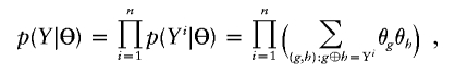and the maximum-likelihood estimate (MLE) of Θ satisfies , where n_g is the count of occurrences of haplotype g in a particular phase configuration Z, and E_Θ(·) means to average over Z under the distribution p(Z|Θ,Y). With Θ^(t) denoting the frequency estimation at the tth iteration, the EM iterates as

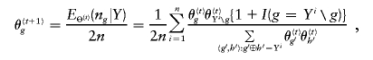where Yⁱ∖g denotes the complement haplotype that pairs with g to make up the genotype Yⁱ, and I(·) is an indicator function. Given the final estimate , we phase the ith individual’s genotype Yⁱ by finding a compatible haplotype pair, (g,h):g⊕h=Yⁱ, that maximizes .

An EM algorithm with probabilistic inputs (EM-II)

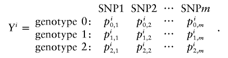
For probabilistic inputs of multiple linked SNPs, such as those resulting from the t-mixture algorithm, the conventional method (EM-I) can no longer be applied. Here, we introduce a new EM-based algorithm, called “GenoSpectrum” (GS)-EM, which can handle such inputs. Let pⁱ_0,k, pⁱ_1,k, and pⁱ_2,k be the likelihood of the ith individual’s FI readouts at marker k, given that its genotype at this marker is heterozygous (Aa, denoted by “0”), wild-type homozygous (AA, denoted by “1”), and variant homozygous (aa, denoted by “2”), respectively. That is, pⁱ_c,k=p{xⁱ_k|yⁱ_k=“c”}=t₂(xⁱ_k;μ_c,k,Σ_c,k,ν), where xⁱ_k represents the FI values of the kth SNP of the ith individual, yⁱ_k represents the genotype at the kth SNP, and t₂(xⁱ_k;μ_c,k,Σ_c,k,ν) is the density function of the bivariate t distribution, with mean μ_c,k, scale Σ_c,k, and known degrees of freedom ν, for cluster “c” (c=0,1,2) at the kth SNP. Note the distinction between the likelihood of the FI values given a cluster, pⁱ_c,k=p{xⁱ_k|yⁱ_k=“c”}, and the posterior cluster (membership) probability, , where w_c is the mixture weight for cluster “c” (see appendix for details). These likelihood vectors for all markers form a 3×m matrix:

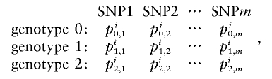where m is the total number of markers in consideration. From this matrix, we can obtain the likelihood of any m-SNP genotype of this individual by multiplying the corresponding single-marker genotype likelihoods under the assumption that the SNPs’ FI readouts are mutually independent. For example, the likelihood for a 3-SNP genotype, Yⁱ=(1,0,2), is

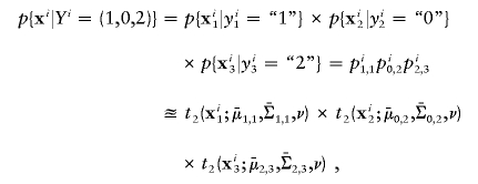where xⁱ represents the FI values of the ith individual, and and are the estimated location and scale parameters of cluster “c” at the kth SNP. Note that this equation is an approximation because the estimated (as opposed to the true) values of the location and scale parameters are used. We order all m-SNP genotypes of the ith individual as Y^i,1,…,Y^i,l_i, with their associated likelihoods π^i,1,…,π^i,l_i, and call

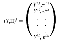the “GenoSpectrum” of the ith individual, where l_i is the number of possible genotypes for the ith individual—that is, those with π^i,j>0. Although there are a total of 3^m possible genotypes for m closely linked biallelic SNP markers, we usually only need to list a small number of the genotypes with nonzero likelihood values.

In situations in which the GenoSpectrum of each individual is available, the likelihood function for haplotype frequencies can be computed as in a typical missing data problem:

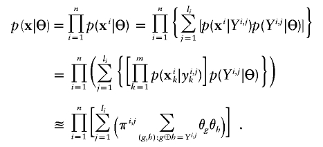From this expression, we are able to obtain the following EM iteration for Θ:

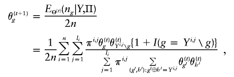where Y^i,j∖g denotes the complement haplotype that pairs with g to make up the genotype Y^i,j. Note that the EM-I algorithm is a special case of the EM-II with l_i=1. The ith individual’s genotype is phased, given the final estimate , by finding a compatible haplotype pair (g,h):g⊕h=Y^i,j that maximizes .

Three phasing strategies based on raw FI values

Three phasing strategies (denoted as “S1,” “S2,” and “S3”) have been used in our study (illustrated in fig. 3):

• S1: clustering step uses the t-mixture model; phasing step uses EM-I algorithm;
• S2: clustering step uses the t-mixture model; phasing step uses EM-II algorithm;
• S3: clustering step uses the t-mixture model with a removal of ambiguous points; phasing step uses EM-I algorithm.

S1 uses the t-mixture model in the clustering step to make deterministic calls (assigning each individual to its most probable cluster) and uses the EM-I algorithm in the phasing step. For example, for a data point with cluster probabilities 0.51, 0.48, and 0.01 of belonging to the AA, Aa, and aa clusters, respectively, S1 will still deterministically assign it to the AA cluster. Although the K-means algorithm can also be applied in the clustering step, we observed that the results obtained by the K-means algorithm were much worse than those based on the t-mixture model in our simulation comparisons (see table 1). We thus drop the K-means algorithm from subsequent analyses. S2 uses the t-mixture model in the clustering step in making probabilistic calls and uses EM-II in the following phasing step (i.e., in S2, EM-II takes GenoSpectrum as an input). S3 is essentially the same as S1, except that it attempts to simulate the human “best guess” strategy commonly practiced by laboratory technicians: when a data point cannot be assigned with a consensus call by two independent readers, it will be set to “missing.” Here, we assume that the independent human readers will not be able to make consensus calls for all ambiguous data points (i.e., a SNP with all the cluster probability values <0.9 cannot be assigned to any of the AA, Aa, or aa genotype clusters.). Thus, all such ambiguous data points of the raw FI data will be removed at this step and not used in the phasing step. For a data point with cluster probabilities 0.51, 0.48, and 0.01 of belonging to the AA, Aa, and aa clusters, respectively, S3 will toss it away. However, for a data point with cluster probabilities 0.045, 0.91, and 0.045 of belonging to the AA, Aa, and aa clusters, respectively, S3 will assign it to the Aa cluster.

Table 1.

Comparison of Clustering Accuracy between the K-Means Algorithm and the t-Mixture Model in Making Deterministic Genotype Calls^[Note]

	% Miscalls for Scenario
Algorithm/Model	LowAmbiguity	MediumAmbiguity	HighAmbiguity
K-means	9.59	8.82	8.82
t-mixture	.03	.30	.72

Note.— For comparison purposes, we generated 100 data sets for each of low, medium, or high ambiguity scenarios. In each data set, the Gaussian mixture model was used in generating 100 data points forming three genotype clusters. For each algorithm, the percentage (%) of miscalls was defined as number of miscalls / total genotype calls.

Simulation Schemes

Comparison of the three phasing strategies

To compare the performances of S1, S2, and S3, we simulated FI data for each SNP such that each genotype cluster’s shape and size are similar to that of the real FI data generated by a standard genotyping machine. For example, each genotype cluster has a center and spreads in two dimensions with a constant variance. Also, we assumed that the genotype distribution of our simulated data conformed to Hardy-Weinberg equilibrium. To assess the performances of S1–S3 for different levels of “difficulty” in clustering, we simulated the low, medium, and high levels of clustering ambiguity on the basis of different variance-covariance matrices of the t distributions (fig. 2B). The ambiguity level is controlled by changing the correlation coefficient (ρ) of the variance-covariance matrix, such that ρ=0.9, 0.75, and 0.6 correspond to low, medium, and high ambiguity levels, respectively. As the ambiguity level increases, the proportion of ambiguous points on the 2-D FI plots increases (fig. 2B). We generated a two-SNP data set consisting of 100 individuals 100 times for each of the 27 different cases (3 ambiguity levels × 3 allele frequencies × 3 LD levels).

Power studies

To find out whether the power of detecting the disease-related haplotype in these tests can be enhanced by considering genotyping uncertainties, we conducted the following haplotype-based case-control association tests. Suppose that the haplotypes consist of two linked SNP markers that are associated with the disease (denoted as “SNP1” with alleles A and a and “SNP2” with alleles B and b). The four haplotypes are AB, Ab, aB, and ab, with haplotype frequencies θ_AB, θ_Ab, θ_aB, and θ_ab, respectively, which satisfy θ_AB+θ_Ab+θ_aB+θ_ab=1. For the hypothetical case-control study, we considered three different models in our simulation experiment, with the frequencies listed as θ_AB, θ_Ab, θ_aB, and θ_ab. These models are (1) case group: 0.4, 0.3, 0.2, 0.1 and control group: 0.25, 0.25, 0.25, 0.25; (2) case group: 0.4, 0.1, 0.1, 0.4 and control group: 0.25, 0.25, 0.25, 0.25; and (3) case group: 0.4, 0.1, 0.2, 0.3 and control group: 0.3, 0.1, 0.4, 0.2. The simulation proceeds as follows:

• 1. Simulate n=100 haplotypes and randomly pair them to obtain 50 individual genotypes in each of the case and control populations, according to each group’s haplotype frequencies.
• 2. Pool all 100 individuals (50 cases + 50 controls) and generate their FI values according to low, medium, and high ambiguity levels.
• 3. Cluster the 100 individuals through use of the t-mixture model and obtain the estimated cluster likelihoods, pⁱ_0,k, pⁱ_1,k, and pⁱ_2,k, as well as the cluster posterior probabilities for each individual and SNP.
• 4. Phase the 100 genotypes (or GenoSpectrums) through use of strategies S1, S2, and S3 and count the number of times each of the four different haplotypes appears in the case and control populations. Record counts in each cell of the 2 (case/control) × 4 (AB/Ab/aB/ab) table. It is also possible to use the expected haplotype counts, as in the EM algorithm.
• 5. Compute the homogeneity test statistic for the 2 × 4 table: (observed count−expected count)²/expected count], where expected count = (row total × column total)/2n.
• 6. 
  Randomize to obtain the critical values:

  • a. 
    Assign individuals randomly to the control and case groups, along with their pⁱ_0,k, pⁱ_1,k, and pⁱ_2,k values obtained in step 3. Redo steps 4 and 5 for this randomly permuted data set.
  • b. 
    Repeat step 6a 500 times and obtain the 90th, 95th, and 99th percentiles of the test statistics, which serve as critical values for significance levels .10, .05, and .01, respectively.
• 7. Record whether the null hypothesis is rejected or accepted by comparing the test statistics of the original simulated data with the critical values from step 6b.
• 8. Repeat steps 1–7 500 times.
• 9. Compute the power of the test—that is, the proportion of times the test was rejected.

Although the test statistic λ has an approximate χ²(3df) distribution under the null hypothesis of no association in the standard situation, we cannot use this property here, because the haplotype counts in the table are not truly observed. Rather, these counts are estimated from the genotype data, which introduces additional uncertainty and may inflate the type I error. As an alternative, we employed a randomization procedure to determine the critical values for a given significant level, as detailed in step 6 above.

Results

Simulation Study for Phasing Accuracy

Comparing the K-means and t-mixture models for genotype scoring

We compared the accuracies of the K-means algorithm and the t-mixture model under low, medium, and high ambiguity levels. To reduce the complexity of the simulation study, we focused on a three-cluster model without the NFS cluster for the FI outputs. In our simulation, bivariate Gaussian distributions were used to generate the FI scatterplots (we also used t distributions for simulating the FI scatterplots, and the results were similar). We fixed centers of the distributions for AA, Aa, and aa clusters at those estimated from a true data set and generated 100 data points from the multinomial distribution with randomly generated cluster probabilities (which results in a wide range of cluster sizes). Then, FI points were scattered given the true cluster indicators and the ambiguity level. We clustered all 100 points through use of both the K-means algorithm and the t-mixture model. The K-means algorithm was implemented using the K-means function in software package R v.1.5.0. We also implemented the K-means algorithm through use of Splus v.5.1 and found that the results were comparable to the R implementation (data not shown).

To make a fair comparison, we assumed that the number of clusters was three and gave the same starting points for the centers of clusters for both algorithms. In the t-mixture model, we picked the cluster with the highest probability. We counted the number of erroneous calls (defined as the calls different from the true calls) in each simulation and repeated this procedure 100 times. At every ambiguity level, the t-mixture model outperformed the K-means algorithm (table 1) by a large margin. One of the reasons for the poor performance of the K-means method is that it had difficulty accommodating the elongated shapes of the FI clusters, because of its use of the standard Euclidean distance. In contrast, the t-mixture model can utilize the shape information by updating the covariance matrix of each component.

In addition to performing poorly, the K-means algorithm also requires correct specification of the number of clusters, which requires the human judgment of “eyeballing” the scatterplot to determine the proper number of clusters before running the program. In contrast, the t-mixture model is not sensitive to the input cluster number, as long as it matches or exceeds the true number (at most 4 in this case). The use of informative priors ensures that the t-mixture model is not sensitive to empty clusters. Examples of obvious mistakes made by the K-means algorithm in the clustering are shown in figure 4. The choice of prior distributions for the t-mixture model will be discussed in the appendix.

Figure 4.

Comparisons of the K-means algorithm and the t-mixture algorithm. Each point (x, y) represents the genotype of an individual, where x and y denote the FI values for the two alleles, respectively. The cluster label is shown for each data point for the ground truth, as well as the clustering results of the bivariate t-mixture model (“t-mix”) and the K-means algorithm. A, A three-cluster example. B, A two-cluster example. Note that the K-means algorithm requires the user to prespecify the number of clusters, whereas the t-mixture algorithm can determine the number of clusters automatically.

Performance comparisons of S1, S2, and S3 in haplotype inference

After excluding the K-means algorithm from further use, we compared the performances of S1, S2, and S3, which all use the t-mixture algorithm in the clustering step. For demonstration purposes, only two SNPs were considered, and both SNPs were assumed to have the same allele frequency distributions (three different minor-allele frequencies were considered: 0.1, 0.3, and 0.5), and haplotype frequencies were generated in such a way that low, medium, and high LDs were found between the two markers (D′ [Lewontin 1964] ranges from 0 to 0.5; 0.5 to 0.75; and 0.75 to 0.95, respectively).

The first step is to specify the “ground truth” haplotype phase. After the haplotype frequencies were chosen according to the allele frequency and the LD rate, 200 haplotypes were drawn randomly, according to their corresponding frequencies. Then, the 200 haplotypes were randomly paired to make 100 hypothetical individual genotypes.

The second step is to simulate raw FI readout data given the individual genotypes. For each marker, 100 pairs of data were generated, which can be translated to a scatterplot containing 100 points representing the FI readout data of the 100 hypothetical individuals on this marker. Note that we did not include the NFS cluster when simulating the FI values. This is a legitimate exclusion because, in real experiments, most NFS points result from blank control samples that are artificially added for experimental convenience to serve as negative controls. Genotyping uncertainties were introduced at three different ambiguity levels: low, medium, and high. That is, an FI data point was generated from a bivariate t distribution with a given center and different covariance matrices according to the ambiguity level. The center vectors and the covariance matrices were based on those estimated from a real data set in the XRCC1 gene study, through use of the t-mixture model.

For frequency estimates, we used the following discrepancy measure (Excoffier and Slatkin 1995; Stephens et al. 2001): , where s denotes the total number of existing haplotypes and θ^true_g and denote the true haplotype frequency and the estimated haplotype frequency, respectively. The results are presented in figure 5. At a low ambiguity level, all three strategies perform similarly. At medium and high ambiguity levels, S2 outperforms both S1 and S3. As we expected, S2 was especially advantageous in high-LD cases. For the phasing of each individual’s haplotypes, S1 and S2 showed comparable accuracies, although, in the case of high LD, S2 outperformed S1 slightly. This is consistent with the result from the frequency estimate. Both S1 and S2 were much more robust than S3 in the high ambiguity case (data not shown).

Figure 5.

Performance comparison of haplotype frequency estimations of the three strategies. The vertical axis measures discrepancy is , the scaled absolute difference between the estimated and the true haplotype frequencies. The error bars are shown as ±1 SE. S1, S2, and S3 represent competing strategies shown in figure 3, and “base” refers to the use of true genotype calls to feed in the EM-based haplotype phasing algorithms. A total of 100 data sets were generated for each calculation, and each simulated data set contained 100 individuals. The gray bar represents low LD (D^′=0–0.5), the hatched bar represents medium LD (D^′=0.5–0.75), and the unshaded bar represents high LD (D^′=0.75–0.95). f = minor-allele frequency.

A Real-Data Example

We applied S1, S2, and S3 to a real genotype data set of four SNPs (C26304T, C26602T, G28152A, and G36189A) located on the XRCC1 gene through use of a TaqMan assay (Han et al. 2003). This data set resulted from a nested case-control study of breast cancer within the Nurses’ Health Study. From this data set, the genotypes of 2,244 individuals (a mix of both cases and controls) were used to derive the overall population haplotype frequencies. We applied S1, S2, and S3 to a subset of 315 subjects (including both cases and controls). Genotyping was performed by bench scientists blinded to case-control status; 10% blinded quality-control samples were inserted and therefore genotyped twice, and the concordance rates among the duplicate samples were found to be 100%. Haplotype inference was performed using the partition-ligation EM (PLEM) algorithm (Qin et al. 2002). A bootstrap-like simulation study demonstrated that the haplotype frequencies estimated by PLEM in the overall sample (with N>2,000) were very close to the “truth” (data not shown), and we thus used this estimate as the “benchmark.” All the results are summarized in table 2. The discrepancy rates (D) for S1, S2, and S3 were 0.03215, 0.0284, and 0.03217, respectively, indicating that S2 performed better than both S1 and S3 in this example.

Table 2.

Comparison of Haplotype Frequency Estimated Using the S1, S2, and S3 Strategies for a Data Set Obtained Using the TaqMan Assay

	Haplotype FrequencyEstimated using Strategyb
Haplotypea	S1	S2	S3	Benchmark Haplotype Frequency Estimatec
0000	.1378	.1377	.1347	.116
0001	.3905	.3948	.3917	.408
0010	.3591	.3592	.3637	.357
0011	.0044	.0000	.0000	.000
0100	.0557	.0557	.0574	.051
1000	.0513	.0507	.0505	.061
1001	.0001	.0001	.0001	.003
1010	.0012	.0018	.0019	.000

^aHere, “0” stands for the major allele and “1” stands for the minor allele.

^bIn this study, four SNP markers (from left to right: C26304T, C26602T, G28152A, and G36189A) in the XRCC1 gene were typed using the TaqMan assay for a subset of 315 individuals out of the overall sample (N=2,244).

^cThe weighted average (case plus control) of haplotype frequency estimates reported by Han et al. (2003). The haplotype frequency estimates of the benchmark were obtained by using PLEM.

Power Comparisons of S1, S2, and S3

The results of power comparison in association tests are presented in table 3. Models 1 and 2 assume that the two SNPs are in perfect linkage equilibrium among the controls, whereas, among the cases, they are in strong LD (model 2 had a stronger LD than model 1). Model 3 mimics a complex disease scenario when the case and the control haplotype distributions differ only slightly. Overall, the haplotype distribution differences are the greatest in model 2. Thus, for each method considered, the power was always the greatest in model 2 (table 3). As we expected, the test using the true genotypes as inputs for the haplotype phasing has the largest power in every scenario, which is likely due to the fact that only phasing uncertainty—but no clustering uncertainty—is present. In low-ambiguity cases, S1, S2, and S3 yielded similar powers. In medium- and high-ambiguity cases, it can be seen that S1 and S2 always outperformed S3 because of the obvious reason that in S3 one throws away information (by removing ambiguous points). For model 2, where the cases have a significant LD compared with the controls, S2 had the greatest power among the three under all ambiguity and significance levels.

Table 3.

Comparison of Power to Detect Disease-Related Haplotypes through Use of Different Haplotype Inference Strategies under Various Disease Models and Disease Prevalences at Different Type I Error Rates

		Power
		Low Ambiguity			Medium Ambiguity			High Ambiguity
Modeland αa	Base	S1	S2	S3	S1	S2	S3	S1	S2	S3
1:
.10	55.6	55.2	56.2	55.4	55.2	56.8	51.4	57	58	54
.05	45	43.6	44	43.4	44.4	44	42.4	46.6	48.2	41
.01	29.2	29.8	29.6	30.4	29.4	29.4	25.6	30.4	28.4	24
2:
.10	85.2	82.8	84.2	82.6	80.8	82	78.6	78.8	81	77.4
.05	75	73.2	74	72.4	72.2	73.4	70.8	68.6	71.2	67.2
.01	55.4	53	53.4	52.8	52.8	54.6	52.4	49.8	51.2	46.6
3:
.10	71.8	68.2	68.8	67.4	67.4	68.4	64.4	64.2	65.2	60.2
.05	56.8	55	55.2	54.4	55.8	54.6	51.2	49	50	49.2
.01	32.6	31.4	32.2	29.8	30.2	28.6	25.6	26.8	26.4	26.2

^aFor the hypothetical case-control study, we considered three different models in our simulation experiment with the frequencies listed as θ_AB, θ_Ab, θ_aB, and θ_ab. These models are (1) case group: .4, .3, .2, .1; control group: .25, .25, .25, .25; (2) case group: .4, .1, .1, .4; control group: .25, .25, .25, .25; and (3) case group: .4, .1, .2, .3; control group: .3, .1, .4, .2. α = type I error rate.

Discussion

We developed a novel clustering algorithm based on the t-mixture model for making genotype calls. Using extensive simulations, we compared the performance of this new algorithm with that of the K-means algorithm. Our findings are in agreement with those of Olivier et al. (2002), who found that the K-means algorithm often placed two centroids within one group of data that would be assigned manually to a single cluster (see fig. 4 for examples). As noted by Olivier et al. (2002), this is particularly apparent when one of the homozygote clusters had only a few data points. A reason for the poor performance of the K-means algorithm is that it cannot incorporate information on the approximate locations of the genotype clusters and cannot handle well the elongated shape of these clusters. The t-mixture clustering method addresses the inherent limitation of the K-means method through use of a Bayesian approach based on the mixture of t distributions and can score genotypes probabilistically, which allows for the incorporation of genotyping uncertainties in subsequent analyses.

In our t-mixture clustering algorithm, users can either include or exclude the NFS cluster beforehand. The reasons for excluding the NFS cluster a priori are as follows: (1) blank control samples are often known to the laboratory technician in advance, and there is no need to classify them (i.e., there is no “ambiguity”); (2) genotyping assays for the vast majority of SNP assays typically have a success rate of >98%, which results in a very small group size for assay failures of real samples, which are visually detectable as belonging to the NFS cluster; and (3) the small cluster size of NFS may result in an unstable estimate of the variance-covariance matrix, which may compromise the performance in some cases. In the case in which the NFS cluster was not well defined, users could apply a simple rule (if we assume that the NFS cluster takes an oval in shape) such as (x-x₀)²/a+(y-y₀)²/b⩽R², where (x₀, y₀) denotes the center for the NFS cluster, a and b control the oval’s shape, and R controls the oval’s spread, all of which can be customized for different FI plots by the human reader. When users choose to include the NFS in running our algorithm, the algorithm outputs the probabilities of each individual belonging to the AA, Aa, aa, and NFS clusters, on the basis of which they can then decide whether to exclude an individual.

Poor separation between genotype clusters always constitutes a problem in genotype scoring. For those ambiguous data points, we demonstrated that throwing away ambiguous individuals clearly results in a loss of information and tends to result in reduced accuracy in haplotype frequency estimation when using deterministic calls. Probabilistic scoring gives rise to more quantitative information and flexibility in the haplotype phasing step and thus can improve the accuracy in haplotype phasing, especially in high-LD and high-ambiguity situations.

The haplotype inference method presented here is formulated for unrelated individuals in random samples of case-control association studies or sib-pair studies without parental data. Although many genotyping errors can be directly resolved in light of parental genotype data, a substantial fraction of errors may still go undetected on the basis of inheritance checking (Douglas et al. 2002). The strategies described here should also be applicable to pedigree data, but modifications of the haplotype inference procedure are necessary. Since it faces the same capacity problem as encountered by the EM algorithm for haplotype inference, the current approach is limited in the number of linked loci, especially when ambiguous marker loci are abundant. The partition-ligation strategy introduced by Niu et al. (2002) can be applied to solve this problem, in which genotyping uncertainties can be addressed at each atomistic unit.

The question of how to best use the haplotype frequencies and phases inferred from the genotype data is still an unsolved issue in case-control epidemiology studies. The classic χ² test is no longer valid, because haplotype counts in both cases and controls are not observed but, rather, are inferred. We used a randomization procedure for the power comparison of the three phasing strategies in case-control studies (table 2). The randomization procedure is a nonparametric means for deriving the threshold for a prespecified type I error and may thus be less powerful compared with a valid parametric test. However, such permutation tests are guaranteed to have the stated significance level and have been a popular method in case-control studies for investigating haplotypic effects (Fallin et al. 2001; Li 2001; Luo et al. 2003; North et al. 2003; Tsai et al. 2003).

In sum, the statistical handling of uncertainties in genotype scoring merits more attention than it has received in the past. The use of formal statistical procedures like ours relieves geneticists of the responsibility of manually determining the correct values of doubtful genotypes and is thus essential for an efficient analysis of high-throughput data. The statistical model presented here is formulated only for SNP markers and is not directly applicable to microsatellite genotyping. However, our algorithms can be straightforwardly generalized to that situation or can be used directly if the microsatellite alleles are binned into two categories using a reasonable allele size cut-off. Although we considered only Taqman, OLA, and MassARRAY, the same strategies developed in this article can be extended to handle data from other experimental platforms, such as florescence-polarization single-base extension and Illumina’s BeadArray technologies, Third Wave’s Invader assay, rolling circle amplifications, and molecular beacons.

The GeneScore and GS-EM (i.e., EM-II) software packages are accessible online, at the authors' Web site.

Appendix: A Fast-Convergent Clustering Algorithm based on the t-Mixture Model

The likelihood function of the bivariate t mixture model is

where x={xⁱ=(x_i,y_i)^′;i=1,…,n} is the set of observed pairs of FI values for a SNP location, C is the number of mixture components, the w_c values are the mixture weights (i.e., 0<w_c<1 for all c=1,…,C and ), and t₂(xⁱ;μ_c,Σ_c,ν) is the probability density function of the bivariate t distribution with location parameter μ_c, scale parameter Σ_c, and known degrees of freedom ν. Since the choice of ν is not critical to the analysis, we set ν=7 as a default choice. In practice, lower degrees of freedom are especially desirable when there are many ambiguous points in the scatterplot of FI values. The number of mixture components, C, is fixed at 4 to represent four clusters: AA, Aa, aa, and NFS (see fig. 2B).

Our algorithm iterates the following two steps and outputs Markov chain samples of the model parameters and the cluster indicator (for each individual) from the desired posterior distribution. First, given current values of the parameters, w^(t)_c, μ^(t)_c, and S^(t)_c for c=1,…,C, we sample the unobserved mixture indicator J^i,(t)=(j^i,(t)₁,…,j^i,(t)_C) for each x_i from Multinomial(1;q^i,(t)₁,…,q^i,(t)_C), where j^i,(t)_c is equal to 1 if xⁱ is assigned to the cth cluster and 0 otherwise, and

the probability that x_i belongs to the cth cluster at the tth iteration. Second, given the current mixture indicator, J^i,(t)=(j^i,(t)₁,…,j^i,(t)_C), we sample the parameters, w^(t+1)_c,μ^(t+1)_c, and S^(t+1)_c for c=1,…,C, from their posterior distribution. Note that, given the mixture index, model fitting is straightforward because the parameters follow a series of standard distributions. We assume the natural conjugate proper prior on the mixture weights, (w₁,…,w_c,)∼Dirichlet(1,…,1), which results in the conjugate posterior distribution

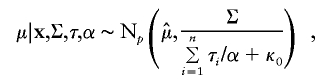
For each cluster, given that we know which cluster each point belongs to from J^i,(t), the sampling of (μ^(t+1)_c,Σ^(t+1)_c) is equivalent to fitting a multivariate t distribution, which can be achieved efficiently using a PXDA scheme (Liu and Wu 1999; van Dyk and Meng 2001) shown at the end of this section.

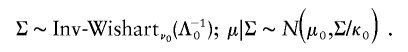
Some difficulties in mixture modeling include the label switching problem (Stephens 2000), the incorrect specification of the cluster numbers, and the occurrences of clusters of small sizes. To make the algorithm stable, we use our prior knowledge of the well-known structure of the FI value scatter plot. First, we use proper priors for the parameter μ_c and Σ_c. Our priors are not proper and are data dependent. They prevent the posterior distribution from being improper even when the data set has an empty cluster. We let the prior distribution of μ_c conditional on Σ_c be N(μ_c0,Σ_c/κ₀), where μ_c0 can be either inputted by the user or defaulted at one of the four “corners” of the data scatterplot, and κ₀ can be chosen by the user (default at 1). The prior for Σ_c is taken as Inv-Wishart_ν0(Λ^-1₀), where Λ₀ is the sample covariance matrix based on all the FI values, and ν₀=p+1, where p=2 is the dimension of the data point. Second, we impose an identifiability constraint on the parameter space of μ_c. Since the general pattern of the scatterplot of FI values contains three clusters away from the origin and one close to the origin, we impose a constraint such that |μ_c|>|μ_NFS|, c=AA, Aa, and aa, and |·| denotes the distance from the origin to the vector. Furthermore, for non-NFS clusters, we impose another constraint that ω_AA>ω_Aa>ω_aa (fig. 2A), where ω_c is the angle of between the vector μ_c and the x-axis. The subscripts indicate the heterozygote cluster (Aa), the homozygote cluster near the x-axis (aa), and the homozygote cluster near the y-axis (AA), respectively.

After the Markov chain of the above posterior sampling scheme has converged, we estimate the likelihood for the ith individual’s FI values at this marker, given that it is in cluster c by , where and are posterior means for the location and scale parameter of the cluster “c.” The reason for using only this value instead of the cluster membership posterior probability is because of the need of computing P(xⁱ|Y^i,j) in the EM-II algorithm. We also compute the posterior mean of the mixture weights, , to compute the cluster membership posterior probabilities for deterministic calls. We repeat this process for all the SNP markers to obtain the matrix representation of the GenoSpectrum of the ith individual:

PXDA for Multivariate t Distribution

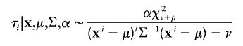
To illustrate the PXDA scheme, we let t_p(μ,Σ,ν) denote the p-dimensional t distribution with center μ, covariance matrix Σ, and known degrees of freedom ν. Note the fact that xⁱ|μ,Σ∼t_p(μ,Σ,ν) is equivalent to xⁱ|τ_i,μ,Σ∼N_p(μ,αΣ/τ_i), and τ_i|μ,Σ∼αχ²_ν/ν, i=1,…,n. The auxiliary scale parameter α is incorporated here to derive a fast-converging Gibbs sampling algorithm. To avoid an improper posterior distribution, we use the conjugate prior distribution for (μ,Σ), which can be parameterized in terms of hyperparameters (μ₀,Λ₀/κ₀;ν₀,Λ₀):

Jointly, we have

According to Liu and Wu (1999), we used Jeffreys’ prior p(α)∝α^-1 for the auxiliary variable. Under this prior specification, we obtain the following sampling scheme:

First, draw

independently for i=1,…,n. Next, draw

and

where Wishart_k(A) denotes the Wishart distribution with scale matrix A and degrees of freedom k. Finally, draw

where

Liu and Wu (1999) showed that the scheme converges to the correct posterior distribution for (μ,Σ), although the posterior distribution of α is still improper. They also proved that the PXDA converges faster than the standard data augmentation scheme and attains the optimal convergence speed when Jeffrey’s prior on α is used.

References

- Abecasis GR, Cherny SS, Cardon LR (2001) The impact of genotyping error on family-based analysis of quantitative traits. Eur J Hum Genet 9:130–134 [DOI] [PubMed] [Google Scholar]
- Akey JM, Zhang K, Xiong M, Doris P, Jin L (2001) The effect that genotyping errors have on the robustness of common linkage-disequilibrium measures. Am J Hum Genet 68:1447–1456 [DOI] [PMC free article] [PubMed] [Google Scholar]
- Akula N, Chen YS, Hennessy K, Schulze TG, Singh G, McMahon FJ (2002) Utility and accuracy of template-directed dye-terminator incorporation with fluorescence-polarization detection for genotyping single nucleotide polymorphisms. Biotechniques 32:1072–1078 [DOI] [PubMed] [Google Scholar]
- Buetow KH (1991) Influence of aberrant observations on high resolution linkage analysis outcome. Am J Hum Genet 49:985–994 [PMC free article] [PubMed] [Google Scholar]
- Clark AG (1990) Inference of haplotypes from PCR-amplified samples of diploid populations. Mol Biol Evol 7:111–122 [DOI] [PubMed] [Google Scholar]
- Dempster AP, Laird NM, Rubin DB (1977) Maximum likelihood from incomplete data via EM algorithm. J Roy Stat Soc Ser B 39:1–38 [Google Scholar]
- Douglas JA, Boehnke M, Gillanders E, Trent JM, Gruber SB (2001) Experimentally-derived haplotypes substantially increase the efficiency of linkage disequilibrium studies. Nat Genet 28:361–364 10.1038/ng582 [DOI] [PubMed] [Google Scholar]
- Douglas JA, Boehnke M, Lange K (2000) A multipoint method for detecting genotyping errors and mutations in sibling-pair linkage data. Am J Hum Genet 66:1287–1297 [DOI] [PMC free article] [PubMed] [Google Scholar]
- Douglas JA, Skol AD, Boehnke M (2002) Probability of detection of genotyping errors and mutations as inheritance inconsistencies in nuclear-family data. Am J Hum Genet 70:487–495 [DOI] [PMC free article] [PubMed] [Google Scholar]
- Excoffier L, Slatkin M (1995) Maximum-likelihood estimation of molecular haplotype frequencies in a diploid population. Mol Biol Evol 12:921–927 [DOI] [PubMed] [Google Scholar]
- Fallin D, Cohen A, Essioux L, Chumakov I, Blumenfeld M, Cohen D, Schork NJ (2001) Genetic analysis of case/control data using estimated haplotype frequencies: application to APOE locus variation and Alzheimer’s disease. Genome Res 11:143–151 10.1101/gr.148401 [DOI] [PMC free article] [PubMed] [Google Scholar]
- Goldstein DR, Zhao H, Speed TP (1997) The effects of genotyping errors and interference on estimation of genetics distance. Hum Hered 47:86–100 [DOI] [PubMed] [Google Scholar]
- Grant SF, Steinlicht S, Nentwich U, Kern R, Burwinkel B, Tolle R (2002) SNP genotyping on a genome-wide amplified DOP-PCR template. Nucleic Acids Res 30:e125 10.1093/nar/gnf125 [DOI] [PMC free article] [PubMed] [Google Scholar]
- Han J, Hankinson SE, De Vivo I, Spiegelman D, Tamimi R, Mohrenweiser HW, Colditz GA, Hunter DJ (2003) A prospective study of XRCC1 haplotypes and their interaction with plasma carotenoids on breast cancer risk. Cancer Res 63:8536–8541 [PubMed] [Google Scholar]
- Hartigan JA, Wong MA (1979) A K-means clustering algorithm. Appl Stat 28:100–108 [Google Scholar]
- Hawley ME, Kidd KK (1995) HAPLO: a program using the EM algorithm to estimate the frequencies of multi-site haplotypes. J Hered 86:409–411 [DOI] [PubMed] [Google Scholar]
- Kirk KM, Cardon LR (2002) The impact of genotyping error on haplotype reconstruction and frequency estimation. Eur J Hum Genet 10:616–622 10.1038/sj.ejhg.5200855 [DOI] [PubMed] [Google Scholar]
- Lewontin RC (1964) The interaction of selection and linkage. I. General consideration; heterotic models. Genetics 49:49–67 [DOI] [PMC free article] [PubMed] [Google Scholar]
- Li H (2001) A permutation procedure for the haplotype method for identification of disease-predisposing variants. Ann Hum Genet 65:189–196 10.1046/j.1469-1809.2001.6520189.x [DOI] [PubMed] [Google Scholar]
- Lin S, Cutler DJ, Zwick ME, Chakravarti A (2002) Haplotype inference in random population samples. Am J Hum Genet 71:1129–1137 [DOI] [PMC free article] [PubMed] [Google Scholar]
- Liu JS, Wu YN (1999) Parameter expansion for data augmentation. J Am Stat Assoc 94:1264–1274 [Google Scholar]
- Livak KJ, Marmaro J, Todd JA (1995) Towards fully automated genome-wide polymorphism screening. Nat Genet 9:341–342 [DOI] [PubMed] [Google Scholar]
- Long JC, Williams RC, Urbanek M (1995) An E-M algorithm and testing strategy for multiple-locus haplotypes. Am J Hum Genet 56:799–810 [PMC free article] [PubMed] [Google Scholar]
- Luo X, Kranzler HR, Zhao H, Gelernter J (2003) Haplotypes at the OPRM1 locus are associated with susceptibility to substance dependence in European-Americans. Am J Med Genet 120B:97–108 [DOI] [PubMed] [Google Scholar]
- Michalatos-Beloin S, Tishkoff SA, Bentley KL, Kidd KK, Ruano G (1996) Molecular haplotyping of genetic markers 10 kb apart by allele-specific long-range PCR. Nucleic Acids Res 24:4841–4843 10.1093/nar/24.23.4841 [DOI] [PMC free article] [PubMed] [Google Scholar]
- Niu T, Qin ZS, Xu X, Liu JS (2002) Bayesian haplotype inference for multiple linked single-nucleotide polymorphisms. Am J Hum Genet 70:157–169 [DOI] [PMC free article] [PubMed] [Google Scholar]
- North BV, Curtis D, Cassell PG, Hitman GA, Sham PC (2003) Assessing optimal neural network architecture for identifying disease-associated multi-marker genotypes using a permutation test, and application to calpain 10 polymorphisms associated with diabetes. Ann Hum Genet 67:348–356 10.1046/j.1469-1809.2003.00030.x [DOI] [PubMed] [Google Scholar]
- Olivier M, Chuang LM, Chang MS, Chen YT, Pei D, Ranade K, de Witte A, Allen J, Tran N, Curb D, Pratt R, Neefs H, de Arruda Indig M, Law S, Neri B, Wang L, Cox DR (2002) High-throughput genotyping of single nucleotide polymorphisms using new biplex invader technology. Nucleic Acids Res30:e53 [DOI] [PMC free article] [PubMed] [Google Scholar]
- Qin ZS, Niu T, Liu JS (2002) Partition-ligation-expectation-maximization algorithm for haplotype inference with single-nucleotide polymorphisms. Am J Hum Genet 71:1242–1247 [DOI] [PMC free article] [PubMed] [Google Scholar]
- Ranade K, Chang MS, Ting CT, Pei D, Hsiao CF, Olivier M, Pesich R, Hebert J, Chen YD, Dzau VJ, Curb D, Olshen R, Risch N, Cox DR, Botstein D (2001) High-throughput genotyping with single nucleotide polymorphisms. Genome Res 11:1262–1268 [DOI] [PMC free article] [PubMed] [Google Scholar]
- Risch NJ (2000) Searching for genetic determinants in the new millennium. Nature 405:847–856 10.1038/35015718 [DOI] [PubMed] [Google Scholar]
- Sobel E, Papp JC, Lange K (2002) Detection and integration of genotyping errors in statistical genetics. Am J Hum Genet 70:496–508 [DOI] [PMC free article] [PubMed] [Google Scholar]
- Stephens M (2000) Dealing with label switching in mixture models. J R Stat Soc Ser B 62:195–809 [Google Scholar]
- Stephens M, Smith NJ, Donnelly P (2001) A new statistical method for haplotype reconstruction from population data. Am J Hum Genet 68:978–989 [DOI] [PMC free article] [PubMed] [Google Scholar]
- Tsai CT, Fallin D, Chiang FT, Hwang JJ, Lai LP, Hsu KL, Tseng CD, Liau CS, Tseng YZ (2003) Angiotensinogen gene haplotype and hypertension: interaction with ACE gene I allele. Hypertension 41:9–15 10.1161/01.HYP.0000045080.28739.12 [DOI] [PubMed] [Google Scholar]
- van den Oord EJ, Jiang Y, Riley BP, Kendler KS, Chen X (2003) FP-TDI SNP scoring by manual and statistical procedures: a study of error rates and types. BioTechniques 34: 610–624 [DOI] [PubMed] [Google Scholar]
- van Dyk D, Meng XL (2001) The art of data augmentation. J Comput Graph Stat 10:1–50 10.1198/10618600152418584 [DOI] [Google Scholar]
- Yan H, Papadopoulos N, Marra G, Perrera C, Jiricny J, Boland CR, Lynch HT, Chadwick RB, de la Chapelle A, Berg K, Eshleman JR, Yuan W, Markowitz S, Laken SJ, Lengauer C, Kinzler KW, Vogelstein B (2000) Conversion of diploidy to haploidy. Nature 403:723–724 10.1038/35001659 [DOI] [PubMed] [Google Scholar]