

Abstract
We consider the probability distribution for fluctuations in dynamical action and similar quantities related to dynamic heterogeneity. We argue that the so-called “glass transition” is a manifestation of low action tails in these distributions where the entropy of trajectory space is subextensive in time. These low action tails are a consequence of dynamic heterogeneity and an indication of phase coexistence in trajectory space. The glass transition, where the system falls out of equilibrium, is then an order–disorder phenomenon in space–time occurring at a temperature Tg, which is a weak function of measurement time. We illustrate our perspective ideas with facilitated lattice models and note how these ideas apply more generally.
Keywords: dynamic heterogeneity, entropy, phase transition, supercooled liquids
A glass transition, where a supercooled fluid falls out of equilibrium, is irreversible and a consequence of experimental protocols, such as the time scale over which the system is prepared and the time scale over which its properties are observed (for reviews, see refs. 1–3). It is thus not a transition in a traditional thermodynamic sense. Nevertheless, the phenomenon is relatively precipitous, and the thermodynamic conditions at which it occurs depend only weakly on preparation and measurement times. In this article, we offer an explanation of this behavior in terms of a thermodynamics of trajectory space.
Our considerations seem relatively general because they are a direct consequence of dynamic heterogeneity (4–6) in glassforming materials. Our primary point is that the order–disorder of glassy dynamics is revealed by focusing on a probability distribution for an extensive variable manifesting dynamic heterogeneity. There are various choices for this variable, depending on the specific system under investigation. We have more to say about this later, but to be explicit about what can be learned, most of this article focuses on kinetically constrained models (7) and the dynamical actions of these models.
We show here that due to the emergence of spatial correlations in the dynamics, i.e., dynamic heterogeneity, action distributions have larger low action tails than what would be expected in a homogeneous system. These tails indicate a coexistence between space–time regions where motion is plentiful and regions where motion is rare. In the latter the entropy of trajectories is subextensive in time, as previously suggested (8). The glass transition, where the system falls out of equilibrium at long but finite observation time, is thus a disorder–order transition in space–time. In contrast with thermodynamic theories of the glass transition (e.g., refs. 9–12), this ordering in trajectory space is not a consequence of any underlying static transition. Further, it follows from our results here that the exponential tails observed in the aging of soft materials, so-called intermittency (refs. 13–15, and see refs. 16–18), are a consequence of dynamic heterogeneity and should be seen in mesoscopic measurements in the equilibrium dynamics of glass formers.
Models and Distributions of Dynamical Activity
We consider two facilitated models of glass formers to illustrate our ideas: the lattice model of Fredrickson and Andersen (FA) (19) in spatial dimension d = 1 and its dynamically asymmetric variant, the East model (20). The FA and East models serve as a caricatures of strong and fragile glass formers, respectively (21, 22). In both cases, there is an energy function JΣini, where J > 0 sets the equilibrium temperature scale, ni is either 1 or 0, indicating whether lattice site i is excited or not, and the sum over i extends over lattice sites. The system moves stochastically from one microstate to another through a sequence of single-cell moves. In the FA model, the state of cell i at time slice t + 1, ni,t+1, can differ from that at time slice t, ni,t, only if at least one of two nearest neighbors, i± 1, is excited at time t. In the East model the condition is that ni+1,t must be excited. These dynamic constraints affect the metric of motion, confining the space–time volume available for trajectories (23). This mimics the effects of complicated intermolecular potentials in a dense nearly jammed material. Excitations in this picture are regions of space–time where molecules are unjammed and exhibit mobility. As such, we refer to ni,t as the mobility field. For both models, the dynamics is time-reversal symmetric and obeys detailed balance. The equilibrium concentration of excitations,  , is the relevant control parameter. The average distance between excitations sets the characteristic length scale for relaxation,
  , and thus the typical relaxation time, τ ≈ c-Δ, where Δ = 3 for the FA model and Δ ≈ -ln c/ln 2 for the East model (see ref. 7 for details).
The total system under consideration has Ntot sites and evolves for ttot time steps, so that the total space–time volume is Ntot× ttot. Within it, we consider a subsystem with spatial volume N and observed time duration tobs, and use x(tobs) to denote a trajectory in that space–time volume. For the FA and East models, this trajectory specifies the mobility field ni,t for 1 ≤ i ≤ N and 0 ≤ t ≤ tobs. The probability density functional for x(tobs), denoted by P[x(tobs)], defines an action,  ; namely,
  . In the FA and East models,
  is a sum over i and t of terms coupling ni,t to mobility fields at nearby space–time points.¶ As such, its average value will be extensive in N× tobs. This extensivity is a general property for any system with Markovian dynamics and short-ranged interparticle forces.
The distribution function for the action is
 |
[1] |
where the pointed brackets indicate average over the ensemble of trajectories of length tobs, and  is the number of such trajectories with action ℰ. When N is much larger than any dynamically correlated volume in space, and tobs is much larger than any correlated period,
 |
[2] |
will be extensive in the space–time volume Ntobs. In this case, the entropy per space–time point,  , will be intensive. Similarly, and for the same reasons, the mean square fluctuation,
 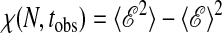 , is extensive for large enough Ntobs. The onset of this extensivity with respect to tobs can be viewed as an order–disorder phenomenon, as we will discuss shortly.
The distribution function for the action can be obtained from simulation by running trajectories and creating a histogram for the logarithm of the probabilities for taking steps in the trajectory. Far into the wings of the distribution, satisfactory statistics is obtained with transition path sampling (25). This methodology allows us to carry out umbrella sampling (26) applied to trajectory space.∥ Fig. 1 illustrates the  we have obtained in this way for the FA and East models. Whereas the bulk of the distributions is Gaussian, for values of the action sufficiently smaller than
  , they display exponential tails. Similar distributions are found for other measures of dynamic activity, such as the number of transitions or kinks in a space–time volume,
 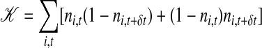 , or the total number of excitations
  . This is shown in Fig. 1 Left Inset.
Fig. 1.

Distribution functions for action and related quantities. (Left) Probability distribution of the action  in the FA model at T = 1, subsystem size
  , and tobs = 320 ≈ 3τ.(Inset) Probability distribution of number of kinks,
  (left and upper axes) and of number of excitations,
  (lower and right axes). (Right)
  but now for tobs = 1,280 ≈ 12τ. The straight line indicates the exponential tail
 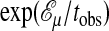 (regime a; see text). (Inset) Coefficient μ at different T from simulation and theory for both the FA and East models. Statistical uncertainties from simulations are smaller than the symbols.
Dynamic Heterogeneity and Susceptibility
Fig. 2 makes vivid the fact that the exponential tails in these distributions are manifestations of dynamic heterogeneity. The extended bubble or stripe in trajectory a of Fig. 2 illustrates a volume of space–time that is absent of excitations. Because it extends throughout the pictured time frame, the statistical weight for this excitation void is dominated by the probability to observe this void at the initial time t = 0. Because excitations at a given time slice are uncorrelated, this probability is Poissonian, exp(-cL), where L is the width of the stripe. In the presence of a bubble occupying a space–time volume Ltobs, the net action is 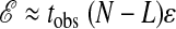 , where ε is the average action per unit space–time. In this regime, the probability density for the action is then
 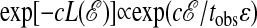 . This proportionality explains why the slope of the exponential tail scales linearly with inverse time. The specific value of that slope is determined from evaluating the action density. Performing the requisite average of the action gives
  c ln c, for small c, where f(c) ≈ 2c for the FA model and f(c) ≈ c for the East model. Hence, to the degree that this picture is correct, the slope μ/tobs in Fig. 1 should coincide with μ = c/ε. Fig. 1 Right Inset shows that this relationship holds to a good approximation. Thus, the exponential tail in
  manifests structures in space–time that depend on initial conditions over a time frame tobs. It also follows that the entropy for trajectories with action that falls in the exponential tails is nonextensive in time tobs.
Fig. 2.

Trajectories in the FA model corresponding to the regimes a, b, and c of Fig. 1. Unexcited and excited sites are colored white and dark, respectively. Space runs along the vertical direction, and time runs along the horizontal direction. Dashed lines delimit the measured space–time volume, N × tobs.
The tails in  are statistically negligible when tobs is large compared with the relaxation time τ, but they are dominant when tobs ≲ τ. The latter regime is where the mean square fluctuation or susceptibility, χ(N, tobs), is nonlinear in time. Fig. 3 Left shows the growth of this quantity with respect to tobs. The susceptibility per unit space–time increases with increasing tobs because increasing time allows for increased fluctuations. With the onset of decorrelation, when tobs > τ, the susceptibility becomes extensive and χ(N, tobs)/Ntobs becomes a constant. This plateau or constant value increases with decreasing T because fluctuations become more prevalent as c decreases. Indeed, the FA and East models approach dynamic criticality as c → 0 (27).
Fig. 3.

Action susceptibility per unit length and time, χ/Ntobs, for the FA model. (Left) This quantity as a function of observation time tobs for constant temperature T, in the FA model. (Inset) Scaled susceptibility, 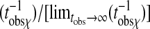 as a function of tobs/τ.(Right) Action susceptibility per unit length and time, χ/Ntobs but now as a function of T at constant tobs.(Inset) Free energies of trajectories,
  , for observation time tobs = 3,200 at different temperatures. System sizes are N = 16c-1. For tobs = 3,200, T* ≈ 0.44. Statistical uncertainties from simulations are smaller than the symbols.
While the plateau value of χ(N, tobs)/Ntobs increases with decreasing T or c, the time for the onset to extensivity also increases. As a result, if tobs is kept fixed and T is varied, χ(N, tobs) will have a maximum. This behavior is illustrated in Fig. 3 Right. The extremum will approach a singularity in the limit of criticality, tobs → ∞, c → 0. For tobs fixed and finite, the extremum is located at a finite temperature, T*, namely, τ(T*) ∼ tobs, where τ(T) denotes the equilibrium relaxation time at the temperature T. Accordingly, T* is a glass transition temperature. In particular, below this temperature, the system cannot equilibrate on time scales as short as tobs. In other words, with observation times no longer than this, the system will have fallen out of equilibrium. For the Arrhenius FA model, ln τ(T) ∝ 1/T, so that T* in this case varies logarithmically with observation time tobs. For the super-Arrhenius East model, ln τ(T) ∝ 1/T2, T* is even more weakly dependent upon observation time, going as  . It is because of this weak dependence on observation time that the glass transition is very nearly a material property, being confined to a narrow range of temperatures.
Similar behaviors are expected for distributions of analogous quantities in continuous force systems. One such quantity is  , where rj(t) refers to the position of the jth particle at time t, and the sum includes all those particles j that are in volume V at time 0. The wave-vector k and time lag δt, while microscopic, should be such that variation in 𝒬 is due to particle diffusion or reorganization and not simply vibrational motion. In the past, studies of dynamic heterogeneity have considered the susceptibility for
  , regarding the time lag δt as a variable that can be large (27, 28). The effect of this variability and the differentiation is to focus on an object that is not extensive in tobs, thus obscuring order–disorder in space–time.
Not all variables extensive in space and time are useful for the type of analysis illustrated here. This situation is familiar in standard phase transition theory. Phase transitions are recognized only through physically motivated choices of variables that are then shown to reflect the transition. For example, consider Langevin dynamics, 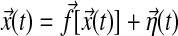 , where
  is a Gaussian random force. In this case, the contribution to the action for a transition in infinitesimal time dt → 0 is, up to a constant,
  , which is distributed as
  independently of the forces
  . The net action for a trajectory is simply the accumulation of these infinitesimal steps and will therefore be distributed in a trivial manner. It is insensitive to the phenomenon we are after. The action for nonlinear functions or functionals of the Langevin
  , however, need not be trivial (see, for example, ref. 29). For variables that manifest dynamic heterogeneity, in particular, a meaningful observable can be constructed out of the probability for finite (not infinitesimal) steps:
  , where δt is an appropriate coarse-graining time. The integrals over intermediate states make the action for finite moves,
  , dependent on the actual forces
  , and the distribution for this action will be system-dependent. The case of deterministic dynamics is similar in that the microscopic action is always vanishing, and a coarse-grained action is needed to reveal interesting behavior. Whether or not this coarse-graining is practical, other variables, such as 𝒬, are clearly useful and practical.
Order–Disorder in Space–Time
Above T*, the system is equilibrated and disordered with respect to order parameters like ℰ or 𝒦 or 𝒬. Below T*, the system is ordered with respect to these quantities, and the order manifests dependence upon initial conditions. In view of the anomalous behavior of χ(N, tobs; T) near T = T*, this dependence can be manipulated in a fashion familiar in the context of equilibrium phase transitions. To this end, it is useful to define 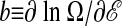 and a corresponding free energy
  . The parameter b is to trajectory space what reciprocal temperature is to state space. In particular, an extremum in χ(T) corresponds with a rapid change in
  with respect to T, which in turn implies a bistable free energy,
  , near b = 1 and T = T*.
Fig. 4 illustrates this behavior. Coexistence takes place at b = b* > 1, the precise value depending on T and tobs. The free energy for b > 1 can be computed from path sampling with a form of thermodynamic perturbation theory (26), running trajectories as before (i.e., with b = 1) and averaging the functional  . In the case illustrated, b* = 1.003, very close to the physical value b = 1. The basin at low action coincides with the exponential tail and, thus, correlation with initial conditions throughout the observed time frame.
Fig. 4.

Free energies of trajectories,  , for different values of the parameter b. The curve for b = 1 is that of Fig. 1 Left, with T = 1, N = 16c-1, and tobs = 320. The curves with b = 1.001, 1.002, and 1.003 are obtained by adding
  to the b = 1 curve. Triangles show the free energy computed by simulation at b = 1.001 using transition path sampling combined with free energy perturbation theory.
For an equilibrium system, b = 1. In this case, there will be a true dynamical singularity for tobs → ∞ only at T = 0. In particular, from the exponential tails of  , we know that b* = 1 + μ/tobs, so that b* → 1 when c → 0 with tobs/τ → finite. An interesting question is whether it is possible to define a dynamical protocol, perhaps through some form of external driving, which would allow one to tune b from b = 1 to b = b* and thus observe this dynamical transition at T > 0.
Acknowledgments
We thank Hans Andersen and Jorge Kurchan for helpful comments on earlier drafts. This work was supported by the National Science Foundation, Department of Energy Grant DE-FE-FG03-87ER13793, Engineering and Physical Sciences Research Council Grants GR/R83712/01 and GR/S54074/01, and University of Nottingham Grant FEF 3024.
Author contributions: M.M., J.P.G., and D.C. performed research and wrote the paper.
Abbreviation: FA, Fredrickson and Andersen.
Footnotes
The microscopic action of either the FA or East models is  . Here, xt ≡ {nit} denotes a configuration at time t, ρ(x0) is the distribution of initial conditions, and
 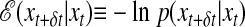 , with p(xt+δt|xt) the probability for an elementary microscopic move in time δt. In a Monte Carlo simulation, for example, δt = 1/N, and the move is an attempted spin-flip. The explicit form of the operator
  is given in ref. 8. Here, we use continuous time Monte Carlo (24), where all attempted moves are accepted: site i is chosen to flip at time t, ni → 1 - ni, with probability (δt)[ni + (1 - ni)e-1/T], and time is increased by δt = (N1f + N0fe-1/T)-1, where N1f and N0f are the number of facilitated up and down sites, respectively, at time t. The corresponding contribution to the action is
  (the last term is added to remove trivial ln N dependences, also present in standard Monte Carlo).
A trajectory of the total system is accepted if the action of the subsystem computed from that trajectory lies between  and
and  . A new trajectory is created from the accepted trajectory by implementing shooting and shifting moves (25). The new trajectory is accepted if the action of the subsystem again lies between
  and
and  , and is rejected otherwise. The ensemble of trajectories created by repeating this process many times provides the distribution function for the action for the subsystem when that action is between
  and
and  . Yet another part of the distribution is created by performing the sampling again, this time for subsystem actions in a different range, say between
  and
and  . Eventually, the distribution is mapped out over the entire range of interest by splicing together many of these partial distributions.
References
- 1.Ediger, M. D., Angell, C. A. & Nagel, S. R. (1996) J. Phys. Chem. 100, 13200-13212. [Google Scholar]
- 2.Angell, C. A. (1995) Science 267, 1924-1935. [DOI] [PubMed] [Google Scholar]
- 3.Debenedetti, P. G. & Stillinger, F. H. (2001) Nature 410, 259-267. [DOI] [PubMed] [Google Scholar]
- 4.Ediger, M. D. (2000) Annu. Rev. Phys. Chem. 51, 99-128. [DOI] [PubMed] [Google Scholar]
- 5.Glotzer, S. C. (2000) J. Non-Cryst. Solids 274, 342-355. [Google Scholar]
- 6.Richert, R. (2002) J. Phys. Condens. Matter 14, R703-R738. [Google Scholar]
- 7.Ritort, F. & Sollich, P. (2003) Adv. Phys. 52, 219-342. [Google Scholar]
- 8.Garrahan, J. P. & Chandler, D. (2002) Phys. Rev. Lett. 89, 035704. [DOI] [PubMed] [Google Scholar]
- 9.Kivelson, D., Kivelson, S. A., Zhao, X., Nussinov, Z. & Tarjus, G. (1995) Physica A 219, 27-38. [Google Scholar]
- 10.Xia, X. & Wolynes, P. G. (2000) Proc. Natl. Acad. Sci. USA 97, 2990-2994. [DOI] [PMC free article] [PubMed] [Google Scholar]
- 11.Franz, S. & Parisi, G. (2000) J. Phys. Condens. Matter 12, 6335-6342. [Google Scholar]
- 12.Bouchaud, J. P. & Biroli, G. (2004) J. Chem. Phys 121, 7347-7354. [DOI] [PubMed] [Google Scholar]
- 13.Cipelletti, L., Bissig, H., Trappe, V., Ballesta, P. & Mazoyer, S. (2003) J. Phys. Condens. Matter 15, S257-S262. [Google Scholar]
- 14.Chamon, C., Charbonneau, P., Cugliandolo, L. F., Reichman, D. R. & Sellitto, M. (2004) J. Chem. Phys. 121, 10120-10137. [DOI] [PubMed] [Google Scholar]
- 15.Ritort, F. (2004) J. Stat. Mech., P10016.
- 16.Bramwell, S. T., Christensen, K., Fortin, J.-Y., Holdsworth, P. C. W., Jensen, H. J., Lise, S., López, J. M., Nicodemi, M., Pinton, J.-F. & Sellitto, M. (2000) Phys. Rev. Lett. 84, 3744-3747. [DOI] [PubMed] [Google Scholar]
- 17.Buisson, L., Bellon, L. & Ciliberto, S. (2003) J. Phys. Condens. Matter. 16, S1163-S1180. [Google Scholar]
- 18.Sibani, P. & Jensen, H. J. (2005) Europhys. Lett. 69, 563-569. [Google Scholar]
- 19.Fredrickson, G. H. & Andersen, H. C. (1984) Phys. Rev. Lett. 53, 1244-1247. [Google Scholar]
- 20.Jäckle, J. & Eisinger, S. (1991) Z. Phys. B 84, 115-124. [Google Scholar]
- 21.Garrahan, J. P. & Chandler, D. (2003) Proc. Natl. Acad. Sci. USA 100, 9710-9714. [DOI] [PMC free article] [PubMed] [Google Scholar]
- 22.Jung, Y. J., Garrahan, J. P. & Chandler, D. (2004) Phys. Rev. E 69, 061205. [DOI] [PubMed] [Google Scholar]
- 23.Whitelam, S. & Garrahan, J. P. (2004) J. Phys. Chem. B 108, 6611-6615. [Google Scholar]
- 24.Bortz, A. B., Kalos, M. H. & Lebowitz, J. L. (1975) J. Comp. Phys. 17, 10-18. [Google Scholar]
- 25.Bolhuis, P. G., Chandler, D., Dellago, C. & Geissler, P. L. (2002) Annu. Rev. Phys. Chem. 53, 291-318. [DOI] [PubMed] [Google Scholar]
- 26.Frenkel, D. & Smidt, B. (2002) Understanding Molecular Simulation (Academic, Boston).
- 27.Whitelam, S., Berthier, L. & Garrahan, J. P. (2004) Phys. Rev. Lett. 92, 185705. [DOI] [PubMed] [Google Scholar]
- 28.Toninelli, C., Wyart, M., Berthier, L., Biroli, G. & Bouchard, J.-P. (2005) Phys. Rev. E 71, 041505. [DOI] [PubMed] [Google Scholar]
- 29.Biroli, G. & Kurchan, J. (2001) Phys. Rev. E 64, 016101. [DOI] [PubMed] [Google Scholar]