An enhanced walrus optimization algorithm for flexible job shop scheduling with parallel batch processing operation

Abstract

The flexible job shop scheduling problem with parallel batch processing operation (FJSP_PBPO) in this study is motivated by real-world scenarios observed in electronic product testing workshops. This research aims to tackle the deficiency of effective methods, particularly global scheduling metaheuristics, for FJSP_PBPO. We establish an optimization model utilizing mixed-integer programming to minimize makespan and introduce an enhanced walrus optimization algorithm (WaOA) for efficiently solving the FJSP_PBPO. Key innovations of our approach include novel encoding, conversion, inverse conversion, and decoding schemes tailored to the constraints of FJSP_PBPO, a random optimal matching initialization (ROMI) strategy for generating diverse and high-quality initial solutions, as well as modifications to the original feeding, migration, and fleeing strategies of WaOA, along with the introduction of a novel gathering strategy. Our approach significantly improves solution quality and optimization efficiency for FJSP_PBPO, as demonstrated through comparative analysis with four enhanced WaOA variants, eleven state-of-the-art algorithms, and validation across 30 test instances and a real-world engineering case.

Introduction

The flexible job shop scheduling problem (FJSP), first explored by Brucker and Schlie¹ and Brandimarte², evolved from the classic job shop scheduling problem (JSP). This problem poses a complex combinatorial optimization challenge involving multiple equalities and inequalities constraints. Due to its wide range of engineering applications and inherent complexity, FJSP has consistently attracted significant research attention^3,4.

The FJSP with parallel batch (p-batch) processing operation (FJSP_PBPO), explored in this study enables multiple jobs to be processed jointly on the same machine, thus posing a challenge to the traditional constraint of the FJSP, where each machine can handle only one job at a time. This problem is motivated by real-world scenarios observed in electronic product testing workshops. In electronic product testing, the workshop devises an overarching testing process plan for prototypes of the same product model. These prototypes are grouped into distinct categories, and each group undergoes sequential testing operations according to specified sub-routes within the plan. Figure 1 illustrates a performance testing process plan for a mobile phone, where 14 prototypes are divided into 7 groups. Each group of prototypes is treated as a single job. However, certain prototypes necessitate cross-group combination testing, leading to parallel batch processing operation (PBPO) on the same machine, as illustrated by (O₁₄, O₂₄) and (O₃₃, O₄₄) in Fig. 1 The introduction of PBPO to the FJSP further complicates the already NP-hard nature of the FJSP^4,5, making it significantly challenging to find viable and optimal solutions, which urgently needs resolution in electronic product testing workshops.

Fig. 1.

Performance testing process plan of the mobile phone.

Recently, swarm-based metaheuristic algorithms have gained significant attention for addressing FJSP due to their efficiency in producing high-quality solutions^6–10. Integrating FJSP_PBPO characteristics with advanced swarm-based metaheuristic mechanisms shows promise for improving optimization in this area. The walrus optimization algorithm (WaOA) is a relatively recent metaheuristic inspired by the behavior of walruses. It is known for its strong exploration capabilities and a balanced approach between exploration and exploitation. This balance allows the algorithm to avoid local optima and effectively explore the solution space, making it particularly well-suited for tackling global optimization problems. However, the algorithm uses a continuous encoding scheme, making it unsuitable for directly solving the FJSP_PBPO addressed in this study. Additionally, the No Free Lunch theorem asserts that no single algorithm is universally effective for all optimization problems, indicating that strong performance on one problem does not guarantee similar results on others¹¹. In industrial applications, the selection, design, and fine-tuning of metaheuristic algorithms must consider the unique demands and characteristics of specific problems to optimize performance effectively¹². Therefore, this study aims to leverage the potential of WaOA and improve it to better address the FJSP_PBPO and enhance its solution quality. The specific innovative contributions are as follows:

1. An optimization model for FJSP_ PBPO is formulated using mixed-integer programming (MIP).

2. An enhanced WaOA (eWaOA) is proposed specifically for FJSP_PBPO.

3. New encoding, conversion, inverse conversion and decoding schemes tailored to FJSP_PBPO are developed.

4. A random optimal matching initialization (ROMI) strategy is designed to generate diverse and high-quality initial solutions.

5. Enhancements to feeding, migration, and fleeing strategies, coupled with the introduction of a novel gathering strategy, enhance the algorithm’s effectiveness in both global exploration and local exploitation.

The subsequent sections are structured as follows: “Related works” section reviews literature on FJSP with p-batch processing and swarm-based metaheuristic algorithms for FJSP. “Description and modeling of FJSP_PBPO” section presents the problem description and model of FJSP_PBPO. “Walrus optimization algorithm” section details the mathematical modeling of WaOA. “The proposed improved WaOA for FJSP_PBPO” section outlines the design of the eWaOA, encompassing encoding, conversion and inverse conversion technique, decoding, population initialization, enhancements of WaOA’s strategies, and newly designed gathering strategy. “Computational experiments and real-word case study” section presents the created benchmark instances, along with the conducted experiments, engineering case study, and results. “Conclusion and future research” section provides the conclusions and the future work.

Related works

FJSP and FJSP with p-batch processing

Since its inception in the beginning of the 90s^1,2, the FJSP has evolved significantly over the past three decades. During this time, researchers have incorporated additional resource constraints, including transport resources^13–16, molds¹⁷, and dual human–machine resources^18,19. Furthermore, new time-related constraints, such as setup times ²⁰ and uncertain processing times^21,22, have been introduced. These advancements continuously broaden the applicability of FJSP, aligning the problem more closely with the optimization demands of real-world workshops⁴. In addition, the FJSP with p-batch processing has also been extensively studied^4,5, with a primary focus on wafer fabrication environments.

According to the standard three-field α|β|γ notation in scheduling, introduced by Graham et al.²³, the FJSP with p-batch processing can be represented as FJ|p-batch |γ, where γ denotes the objective to be optimized. The objectives in these studies mainly include minimizing makespan (C_max), total weighted tardiness (TWT), total tardiness (TT), total completion time (TC), total weighted completion time (TWC), maximum lateness (L_max), maximum tardiness (T_max), and number of tardy jobs (NTJ).

Many studies have proposed heuristic methods based on disjunctive graph (DG), with the most widely explored being variations of the shifting bottleneck heuristic (SBH) initially introduced by Adams et al.²⁴. Mason et al.^25,26 presented a modified SBH to address the FJ| p-batch |TWT. Experimental results show that their modified SBH outperforms dispatching rules and surpasses an MIP heuristic in all but small instances. To reduce computational costs, Mönch and Drießel^27,28 adopted a two-layer hierarchical decomposition approach, using a modified SBH²⁷ and a SBH enhanced by a genetic algorithm (GA)²⁸ for sub-problems optimization. Mönch and Zimmermann²⁹ further applied the SBH to the same problem in a multi-product setting. Barua et al.³⁰ developed a SBH to optimize L_max, TT, TC of the problem within a stochastic and dynamic environment using discrete-event simulation, demonstrating superior performance compared to traditional dispatching methods. Upasani et al.³¹ streamlined the problem by focusing on bottleneck machines in the DG while representing non-bottlenecks as delays, effectively balancing solution quality and computational effort. Sourirajan and Uzsoy³² introduced a SBH that employs a rolling horizon approach to create manageable sub-problems. Upasani and Uzsoy³³ further integrated this rolling horizon strategy with the reduction approach proposed by Upasani et al.³¹. Pfund et al.³⁴ expanded the SBH to optimize TWT, C_max, and TC, employing desirability functions to evaluate criteria at both the sub-problems and machine criticality levels. Yugma et al.³⁵ proposed a constructive algorithm for a diffusion-area FJSP, incorporating iterative sampling and simulated annealing (SA), which demonstrated effectiveness on real-world instances. Knopp et al.³⁶ introduced a new DG and a greedy randomized adaptive search procedure (GRASP) metaheuristic combined with SA, yielding excellent results on benchmark and industrial instances. Ham and Cakici^37,38 developed an enhanced optimization model employing MIP and constraint programming (CP) for the FJ| p-batch |C_max, which was solved using IBM ILOG CPLEX. The computational results demonstrate that the proposed MIP model significantly reduces computational time compared to the original model, while the CP model outperforms all MIP models. Wu et al.³⁹ introduced an efficient algorithm based on dynamic programming and optimality properties for scheduling diffusion furnaces. The developed algorithm not only surpasses human decision-making but also enhances productivity compared to existing methods.

The FJ|p-batch |γ has also been investigated across various other industrial environments. Boyer et al.⁴⁰ investigated this problem in seamless rolled ring production, where jobs are processed in batch furnaces, often in a first-in, first-out sequence, resulting in a PBPO structure. Zheng et al.⁴¹ examined the JSP with p-batch processing, inspired by practical military production challenges, and proposed an auction-based approach combined with an improved DG for solution optimization. Xue et al.⁴² developed a hybrid algorithm integrating variable neighborhood search (VNS) with a multi-population GA to address this problem, validated in a heavy industrial foundry and forging environment. Ji et al.⁴³ constructed a novel multi-commodity flow model for the FJ|p-batch |C_max, introducing an adaptive large neighborhood search (ALNS) algorithm with optimal repair and tabu-based components (ALNSIT) to effectively solve large-scale instances.

The above research provides valuable references for this study. However, existing optimization methods for FJSP with p-batch constraints are challenging to apply directly to the scheduling requirements of electronic product testing workshops. The main reasons are as follows: (1) Most of the research above, particularly studies on wafer fabrication scheduling, primarily focuses on batch processing machines (BPMs) scheduling and multi-level local optimization. In contrast, electronic product testing requires integrated scheduling of all jobs and machines throughout the workshop. (2) Except for the studies by Xue et al.⁴² and Ji et al.⁴³, the process plans of all jobs are similar, and all jobs require processing through BPMs (e.g., acid bath wet sinks, heat treatment machines). In contrast, in this study, job process plans vary significantly, and only the jobs forming the PBPO need to undergo specified p-batch processing in the BPMs. (3) In existing studies, batch processing decisions are dynamically made based on each job’s ready time and the capacity of the BPMs. In contrast, p-batching in this study pertains to specific operations from different jobs that must be processed jointly according to a predefined testing process plan.

Swarm-based metaheuristic algorithms for FJSP

Swarm-based metaheuristic algorithms are inspired by the collective behaviors observed in natural phenomena among mammals, birds, insects, and other organisms. Prominent examples include particle swarm optimization (PSO) (PSO)⁴⁴, ant colony optimization (ACO)⁴⁵, and artificial bee colony (ABC)⁴⁶, which are considered classical swarm-based metaheuristic algorithms. These algorithms have been extensively applied to the FJSP. For instance, Ding and Gu developed an enhanced PSO for addressing the FJSP⁴⁷. Shi et al.⁴⁸ proposed a two-stage multi-objective PSO to tackle a dual-resource constrained FJSP. Zhang and Wong⁴⁹ addressed the FJSP in dynamic environments using a fully distributed multi-agent system integrated with ACO. Li et al.⁵⁰ introduced a reinforcement learning (RL) variant of the ABC for the FJSP with lot streaming.

In the past decade, swarm-based metaheuristic algorithms have seen rapid development, with new algorithms continually emerging. Notable examples include grey wolf optimization (GWO)⁵¹, whale optimization algorithm (WOA)⁵², satin bowerbird optimizer (SBO)⁵³, emperor penguin optimizer (EPO)⁵⁴, squirrel search algorithm (SSA) ⁵⁵, harris hawks optimization (HHO)⁵⁶, red deer algorithm (RDA)⁵⁷, tuna swarm optimization (TSO)⁵⁸, remora optimization algorithm (ROA)⁵⁹, African vultures optimization algorithm (AVOA)⁶⁰, white shark optimizer (WSO) ⁶¹, WaOA⁶², and walrus optimizer (WO)¹². Some of these algorithms provide novel approaches for addressing (F)JSP.

Luo et al.⁶ introduced an advanced multi-objective GWO (MOGWO) aiming at minimizing both makespan and total energy consumption for the multi-objective FJSP (MOFJSP). Lin et al.⁶³ introduced a learning-based GWO tailored for stochastic FJSP in semiconductor manufacturing. It employs an optimal computing budget allocation strategy to enhance computational efficiency and adaptively adjust parameters using RL.

Liu et al.⁷ combined the WOA with Lévy flight and differential evolution (DE) strategies to tackle the JSP. The Lévy flight boosts global search and convergence during iterations, while DE enhances local search capabilities and maintains solution diversity to avoid local optima. Luan et al.⁶⁴ proposed an improved WOA (IWOA) for the FJSP, focusing on minimizing makespan. The IWOA features a conversion method to translate whale positions into scheduling solutions and employs a chaotic reverse learning strategy for effective initialization. Additionally, it integrates a nonlinear convergence factor and adaptive weighting to balance exploration and exploitation, and incorporates a VNS for enhanced local exploitation.

Ye et al.⁸ addressed the FJSP with sequence-dependent setup times and resource constraints by introducing a self-learning HHA (SLHHO) aimed at minimizing makespan. The SLHHO employs a two-vector encoding for machine and operation sequences, introduces a novel decoding method to handle resource constraints, and uses RL to intelligently optimize key parameters. Lv et al.¹⁰ developed an enhanced HHO for both static and dynamic FJSP scenarios. This enhanced algorithm incorporates elitism, chaotic mechanisms, nonlinear energy updates, and Gaussian random walks to reduce premature convergence.

Fan et al.⁶⁵ introduced the genetic chaos Lévy nonlinear TSO (GCLNTSO) for the FJSP with random machine breakdowns, focusing on minimizing a combined index of maximum completion time and stability. He et al.⁶⁶ developed an improved AVOA for the dual-resource constrained FJSP (DRCFJSP). Enhancements to the AVOA include employing three types of rules for population initialization, establishing a memory bank to store optimal individuals across iterations for improved accuracy, and implementing a neighborhood search operation to further optimize makespan and total delay. Yang et al.⁹ developed a hybrid ROA with VNS aimed at optimizing FJSP makespan. The algorithm incorporates a machine load balancing-based hybrid initialization method to enhance initial population quality and a host switching mechanism to improve exploration capabilities.

The advancements in FJSP research and engineering applications are notable, but the existing studies did not address PBPO constraints, which limits their applicability to FJSP_PBPO. Thus, new research is required to integrate the unique aspects of FJSP_PBPO with the selected swarm-based metaheuristic algorithms.

Description and modeling of FJSP_PBPO

The FJSP_PBPO extends the classic NP-hard problem FJSP⁵. It involves processing N jobs on M machines, with each job following a specific process plan composed of sequentially ordered operations. Each operation can be executed on a set of alternative machines with defined processing times. Additionally, some machines can process multiple operations from different jobs simultaneously, subject to PBPO constraints. The primary objective of the FJSP_PBPO is to determine the optimal processing order of each “task” (encompassing both operations and PBPO) on each machine to minimize the makespan (C_max), while also respecting precedence relationships among operations within the same job and among tasks on the same machine. Building on the complexities of FJSP, FJSP_PBPO further increases problem intricacy by incorporating PBPO constraints. Table 1 presents an example of an FJSP_PBPO scenario with four jobs and four machines, where the values under each machine indicate the processing time for each task. As with FJSP, FJSP_PBPO assumes that:

1. All jobs can start processing at time 0, and all the jobs have the same priority.

2. All machines are available at time 0.

3. Each machine can handle only one task at a time.

4. Each job is processed on only one machine at a time.

5. Once a task begins on a machine, it must be completed without interruption.

6. Each task can only start processing after its preceding tasks have been completed.

7. All operations that form the PBPO must start and finish simultaneously.

Table 1.

Instance of FJSP_PBPO.

Jobs	Tasks	Alternative machines
		M1	M2	M3	M4
J1	O11	5	–	7	–
	O12	5	–	–	–
	O13	10	–	12	–
	O14	14	13	–	14
J2	O21	8	–	7	10
	O23	5	7	–	5
J3	O31	4	7	6	–
	O32	8	12	–	–
	O34	5	–	3	5
J4	O41	–	4	–	7
	O42	6	–	7	–
	O44	–	12	–	8
J2, J3	{O22, O33}	7	4	–	–
J2, J4	{O24, O43}	5	3	6	–

J_i represents job i, O_ij represents the jth operation of J_i, {O₂₂, O₃₃} and {O₂₄, O₄₃} are two PBPOs.

The FJSP_PBPO is defined using specific notations. Below, we provide a concise overview of these notations and the corresponding problem formulations.

M: total number of machines;

N: total number of jobs;

m: machine index;

: the task set for all the jobs;

: task index,;

: the immediate job predecessor task(s) of ;

: the processing time of task on machine m;

: the processing time of task ;

: the completion time of task ;

: the corresponding processing time of specific operation on machine m;

: the start time of specific operation ;

: the completion time of specific operation ;

: the completion time of the last task on machine m;

: makespan;

: a sufficiently large integer;

: decision variable representing whether task u is processed on the machine m;

: decision variable representing the order of two different tasks processed on the same machine;

Based on this, an optimization model is constructed using MIP, with the objective of minimizing the maximum completion time.

1

Subject to:

2

3

4

5

6

7

8

Equation (1) represents the optimization objective function. Equation (2) indicates that tasks cannot be interrupted during processing. Equation (3) states that each task can only be processed on one machine. Equation (4) ensures that the completion time of any task does not exceed the maximum completion time . Equation (5) ensures the precedence order between tasks on the same machine. Equation (6) guarantees the precedence order between tasks of the same job. Equation (7) asserts that the start and completion time of any task is non-negative. Equation (8) specify that the various operation of task u must start and finish simultaneously.

Walrus optimization algorithm

In WaOA, each walrus serves as a candidate solution in the optimization problem. Therefore, the position of each walrus within the search space determines the candidate values for the problem variables. The optimization process begins with a population of randomly generated walruses X, representing by D-dimensional random vectors, as defined by Eq. (9).

9

where, is the pth initial walrus (candidate solution), lb and ub are the lower and upper boundaries of the problem, rand is a uniform random vector in the range 0 to 1, is the value of the jth decision variable of the initial walrus , P is the number of walruses in the population, i.e., the population size, D is number of decision variables. Based on the suggested values for the decision variables, the objective function of the problem can be evaluated, and the resulting fitness function can be obtained.

Walruses are agents that perform the optimization process. Their positions are iteratively updated using feeding, migration, fleeing strategies until a termination condition is met. Each iteration follows a structured approach divided into three phases. In Phase 1, the WaOA utilizes feeding strategy to explore globally. In this phase, the best candidate solution so far is identified as the strongest walrus according their fitness. Other walruses adjust their positions under the guidance of according to the Eqs. (10) and (11).

10

11

where is the new position for the pth walrus on the jth dimension, is the current position for the pth walrus on the jth dimension, rand_p,j is a random number lies in the range (0,1), is the position for the strongest walrus on the jth dimension, is an integer selected randomly between 1 or 2.

In Phase 2, each walrus migrates to a randomly selected walrus position in another area of the search space and the new position for each walrus can be generated according to Eqs. (12) and (13).

12

13

where and is the position of the selected walrus to migrate the pth walrus towards it, is its jth dimension, and is its objective function value.

In Phase 3, the WaOA utilizes fleeing strategy to adjust the positions of each walrus within its neighborhood radius. This strategy is used to exploit the problem-solving space around candidate solutions. The new position can generate randomly in this neighborhood using Eqs. (14) and (15).

14

15

where and are the lower and upper bounds of the jth position, respectively, and are allowable local lower and upper bounds for the jth position, respectively. The pseudocode for WaOA is shown in Algorithm 1.

Algorithm 1.

Walrus optimization algorithm (WaOA).

The proposed improved WaOA for FJSP_PBPO

Framework of the eWaOA

Due to the introduction of new constraints by FJSP_PBPO, existing encoding, conversion, and decoding methods for swarm-based metaheuristics used in FJSP are not directly applicable. Consequently, we first develop new encoding, conversion, inverse conversion and decoding schemes tailored to these constraints. Preliminary experiments have identified several shortcomings of the original WaOA when applied to FJSP_PBPO, such as premature convergence to local optima and inefficient updates. To address these issues, this study first create new initialization strategy and then enhance the WaOA’s feeding, migrating, and fleeing strategies. Additionally, a gathering strategy is introduced to enhance both global and local optimization capabilities. The framework for the proposed eWaOA is illustrated in Fig. 2 and detailed below.

Fig. 2.

Flowchart of the proposed eWaOA for the FJSP_PBPO.

Step 1—Data input: Operation set, operation sequence for the N jobs, alternative machines with their associated processing times for each operation, and the PBPOs, with both operations and PBPOs collectively described as tasks.

Step 2—Parameter setting: Population size (P) of walruses, termination parameter (maximum iterations maxT or time limit T), control factor A, and matching parameter K for ROMI.

Step 3—Population initialization: The optimization process begins with P randomly generated walruses based on the ROMI strategy according to the parameter K. Each walrus is encoded as a real vector and an integer vector . On this basis, segmented conversion are developed to convert the to , while the inverse conversion method is created to transform the into . The are decoded using a designed semi-active decoding method to generate feasible scheduling scheme.

Step 4—Update the position of each walrus. Walruses serve as search agents in the optimization process, with their positions continuously updated through enhanced feeding, migration, fleeing strategies, or through the enhanced feeding and introduced gathering strategy. The decision between choosing the gathering strategy or the migration and fleeing strategies is controlled by A. For the feeding, migration, and fleeing strategies, real vectors X are updated directly during each iteration, with simultaneous conversion of the updated real vector into corresponding integer vector . Conversely, gathering strategy involve direct updates of to generate , followed by inversely converting it to corresponding . This ensures synchronization in updating the X and at each iteration.

Step 5—Updating the strongest walrus: Each are decoded into a feasible semi-active schedule for FJSP_PBPO, and the fitness values of the walruses is assigned the reciprocal of makespan corresponding to the schedule. And the walrus with the highest fitness so far is update as the strongest walrus .

Step 6—Termination criterion: If the iterations reaches its preset maxT or the runtime reaches its preset T, the best solution is output, and the iteration stops; else, it proceeds to Step 4.

Representation of walrus and FJSP_PBPO

In our eWaOA, a vector is represented as a D-dimensional real vector, constrained by the specific requirements of the problem. FJSP_PBPO involves two sub-problems: task sequencing and machine assignment. Therefore, X_p should encompass information from both aspects. Let TN denote total number of all tasks in the FJSP_PBPO, then D = 2TN. The first half part of represent task sequencing, while the second half part describes machine assignment for each task. Specifically, denotes the value of the jth task decision variable in the vector , represents the machine assignment decision variable for the (j-TN)th task of . The is defined as the real sub-vector for task (RVT) and is defined as the real sub-vector for machine assignment (RVM) in this study. Additionally, the value of is bound to be in the real range (-N, N), where N is the total number of jobs.

The WaOA is designed for continuous functions but is not directly applicable to discrete problems such as FJSP_PBPO. Additionally, the presence of PBPO implies that a single position in may correspond to multiple operations across different jobs. Consequently, decoding into a feasible schedule and evaluating the objective function value presents significant challenges. To address these issues, we further propose a task-based encoding method for FJSP_PBPO. This encoding scheme consists of an integer vector divided into two parts. The first part, the integer sub-vector for tasks (IVT), represents each position with job ID(s). To maintain consistency, the number of elements in each position is set to , and the length of the vector is set to the number of tasks (TN), where is the number of operations in the k-th PBPO. Positions with fewer than s elements are padded with zeros. If a position contains more than one job ID, it indicates that the position corresponds to a PBPO. For simplicity, padded zeros are omitted in the subsequent description. The second part, the integer sub-vector for machine assignment (IVM), has positions with potential values ranging from 1 to M. Each position in IVM corresponds to the processing machine for the task indicated by the same position in IVT. Figure 3 illustrates the integer vector code for FJSP_PBPO, showing the specific operations or PBPOs in IVT and their corresponding processing times. Thus, each walrus contains both continuous encoding vector and integer vector .

Fig. 3.

An instance of two integer sub-vectors code for the FJSP_PBPO.

Conversion and inverse conversion scheme

The conversion process transforms a real vector to integer vector, allowing the eWaOA to solve FJSP_PBPO. The ranked order value (ROV) rule, originally designed for FJSP or JSP, uses order relationships and random keys to map a real vector into an integer operation sequence, which outlines the order of operations on all machines and forms a scheduling scheme^7,65. However, the inclusion of PBPO in the FJSP_PBPO renders the traditional ROV method unsuitable. To address this, a novel segmented conversion algorithm is developed to convert the real vector into integer vector . This algorithm introduces a task template (TP) segmented into three sections: the first section corresponds to tasks from jobs without PBPO; the second section consists of sequential PBPO tasks; and the third section includes tasks from jobs with PBPO, excluding the PBPOs themselves. For each segment, elements in the RVT are categorized and converted based on the methods outlined in Table 2 ensure that the constraints are maintained. Additionally, when converting the RVM to the IVM, the machine index for each task must be determined first, with the conversion formula provided in Eq. (16):

16

where N denotes the number of jobs, TN represents total number of all tasks, indicates the total number of alternative machines for the task . The segmented conversion algorithm is described as follows:

Algorithm 2.

Segmented conversion.

Table 2.

Categorization and post-processing strategy of a RVT.

B and C represent the values of PBPOs. A is the value of either a job predecessor, successor of B, or the middle task between A and B. N denotes the number of jobs.

Figure 4 illustrates an example of the segmented conversion process from RVT to IVT. First, the task template TP is created with three sections according to the job process plan: the first section, from to , contains tasks for jobs without PBPO; the second section consists of sequentially arranged PBPO tasks and ; and the third section, from to , includes tasks for jobs with PBPO but excludes the PBPOs themselves. The RVT is divided into three sections according to the TP structure, and its elements of RVT is copy to CRVT. Next, related values in the second and third sections of the CRVT are updated according to the conversion formulas given in Table 2. In this example, since O₂₂ in {O₂₂, O₃₃} is a predecessor of O₂₄ in {O₂₄, O₄₃}, the value 3.28 in RVT for {O₂₂, O₃₃} is initially converted to -0.03 in CRVT using the “Predecessor” conversion formula. Subsequently, the “Predecessor”, “Middle”, and “Successor” conversion formulas are applied sequentially to convert the predecessor tasks for {O₂₂, O₃₃} and {O₂₄, O₄₃}, as well as the tasks O₂₃ (middle of the two PBPOs) and the successor tasks. The original RVT values and their converted counterparts in the CRVT for the example in Table 2, are highlighted in red in Fig. 4 Finally, the ranked values of each element in the CRVT are obtained to generate the ROV vector. Following the ascending order of the ROV vector, job IDs are sequentially copied from corresponding positions in the TP to construct the IVT.

Fig. 4.

Example of the segmented conversion from RVT to IVT.

The inverse conversion is designed to transform to while ensuring that the updates of remains consistent with the update of . When converting the IVT to the RVT, a randomly generated RVT is introduced, and the ROV is determined based on the TP and IVT. Then, the RVT is reordered according to the ROV, and the corresponding values in RVT are updated based on the categorization strategies in Table 3, forming the new RVT. When converting IVM to RVM, the value corresponding to each task are first obtained using the following Eq. (17).

17

where is the machine index of the th task, the mean of N, TN and consistent with those in Eq. (16). This inverse conversion process is detailed in Algorithm 3.

Algorithm 3.

Inverse conversion.

Table 3.

Categorization and post-processing strategy of a RVT for inverse conversion.

Figure 5 illustrates an example of the inverse conversion from IVT to the RVT. First, the positions of each TP element within the IVT are recorded to construct the ROV vector. For instance, the 12th and 7th elements of TP, with values (4, 1) and (2, 1) respectively, rank first and second in the IVT. Consequently, the 12th and 7th positions in the ROV vector are assigned the values 1 and 2, respectively. Next, a Reordered RVT is generated by sorting the RVT according to the ROV vector. For example, as shown in the figure, the first and second elements of the ROV vector are 3 and 5, respectively, so the third and fifth elements of the RVT are placed into the first and second positions of the Reordered RVT. Subsequently, the values in the Reordered RVT are converted according to the strategies outlined in Table 3 to generate NewRVT. The conversion process first applies to non-PBPO predecessor tasks, O₂₃ (between the two PBPOs {O₂₂, O₃₃}, {O₂₄, O₄₃}), as well as the successor tasks for both PBPOs. Then, the conversion is performed for {O₂₂, O₃₃}, the predecessor tasks for {O₂₄, O₄₃}. The red-highlighted text in the Reordered RVT and NewRVT in Fig. 5 indicates the corresponding values before and after the inversion conversion, as shown in Table 3.

Fig. 5.

Example of the inverse conversion from IVT to RVT.

Semi-active decoding

Bierwirth and Mattfeld⁶⁷ introduced decoding methods that transform encoded permutations into semi-active, active, non-delay, and hybrid schedules. Among these, the semi-active schedule is particularly straightforward to implement, provides high decoding efficiency, and frequently produces high-quality solutions. Therefore, the semi-active decoding is adopt to decode the for a walrus. This decoding approach ensures that each task adheres to the precedence constraints both within the same job and on the same machine. However, for the FJSP_PBPO, it is crucial to thoroughly evaluate the completion times of all predecessors for each job in the PBPO. The constraints considered during the decoding process become more complex. The specific semi-active decoding designed for FJSP_PBPO is outlined in Algorithm 4.

Algorithm 4.

Semi-active decoding.

Random optimal matching-based initialization

To quickly obtain high-quality initial solutions, it is necessary to comprehensively balance the quality and diversity of the initial population during the initialization. For the optimization of FJSP_PBPO, the quality of the corresponding initial population is related to the matching of task and machine assignment. Based on this, a ROMI method is proposed to initialize the population. Specifically, for each walrus in the first half of the population, one RVT and K RVM are generated randomly accordingly to , , respectively, where N is the number of jobs. Then, segmented conversion and semi-active decoding are employed to determine the makespan of the matched and , and the pair of RVT and with the smallest makespan is selected to initialize .

Conversely, for each walrus in the second half of the population , K RVT and one RVM are generated randomly accordingly to , , respectively. Similarly, the pair of and RVM with the smallest makespan is selected to construct . Since the RVT in the first half and the RVM in the second half of the population are generated randomly, the randomness and diversity of the initial population generation are ensured.

Enhanced feeding strategy

In the original feeding strategy of WaOA, each walrus moves toward the strongest individual in the population. And a random number rand_p,j within the interval (0,1) controls how each dimension of a walrus approaches the , limiting the solution space. Preliminary experiments indicate that when solving the FJSP_PBPO, walruses often get stuck in local optima and experience a slower convergence speed. To enhance the global search capability and efficiency of WaOA, Lévy flight⁶⁸ is incorporated into the feeding strategy. Many animals, including walruses, perform fine-grained searches within a localized area for a period, followed by longer movements to explore other regions. Lévy flight, which alternates between short-distance searches and occasional long-range moves, effectively models this behavior and aligns well with the natural feeding patterns of walruses. The feeding strategy, now integrated with Lévy flight for updating walrus positions, can be expressed by modifying the previous formula as follows:

18

where sign [rand − 0.5] can take one of three values: − 1, 0, or 1. ⊕ means entry wise multiplication.

Lévy flight is a kind of non-Gaussian random process, and its step length obeys a Lévy distribution.

19

where s represents the step length of the Lévy flight, and β is an index parameter. The value of s can be calculated using Mantegna’s algorithm as follows:

20

where β is set to be 1.5, and both μ and v follow normal distributions.

21

where Γ denotes the standard Gamma function. According to Eqs. (18)–(21), Eq. (18) can be reformulated as:

22

Enhanced migration strategy

In the original migration strategy of the WaOA, each walrus randomly selects another walrus from the population as its migration destination. Throughout the iteration process, the updates of the walruses lack an adaptive adjustment mechanism, leading to slower convergence speeds or entrapment in local optima. To enhance global exploration in the early stages and strengthen local exploitation in the later stages of iteration, the migration strategy of WaOA is modified by introducing a self-adjusting factor C to replace rand in Eq. (12). The position update formula for walrus can then be rewritten as:

23

24

where t denotes the current iteration number and T represents the maximum number of iterations. In the early stages, when t is relatively small, the value of C is large, allowing individuals to explore with a greater step size during position updates. This facilitates rapid coverage of a broader search space and enhances global exploration. As the iterations progress, t gradually increases while C decreases. In the later stages, a smaller value of C promotes fine local exploitation within these improved regions, enhancing the algorithm’s convergence efficiency.

Enhanced fleeing strategy

The original update expression for the fleeing strategy is shown in Eqs. (14) and (15). However, the local lower bound and upper bound in the Eq. (14) is controlled by the inverse proportional function and respectively. The inverse proportional function prioritizes global exploration at the beginning of the algorithm’s iterations, with a larger radius to discover optimal regions within the search space. However, the neighborhood radius of the inverse proportional function decays rapidly, leading to a quick decline in global exploration capability, which makes it difficult for the fleeing strategy to play an exploitation role in the later stages of the algorithm. Therefore, this study replaces the original inverse proportional function with an arctangent function to control the local bound in fleeing. Then the fleeing strategy can be mathematically modelled by the Eq. (25).

25

where the mean of t and T consistent with those in Eq. (24).

Gathering strategy

Walruses enhance their foraging and movement efficiency by interacting and sharing location information with one another. To model this behavior, we propose a “gathering strategy” in which walruses form pairs and exchange information, thereby improving the herd’s ability to identify areas with higher food availability. To assess this information-sharing process, walruses are paired through a random selection method. Based on these paired walruses, such as X_p^'t and , the position of each individual is updated according to the following Algorithm 5.

Algorithm 5.

Gathering strategy.

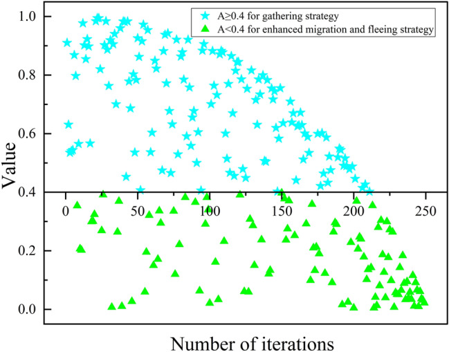
A control factor, denoted as A, is introduced to regulate the population’s updating strategy. If A reaches or exceeds 0.4 after the feeding strategy, walruses will adopt migration, fleeing strategies to explore and exploit search area. Conversely, if A falls below 0.4, a gathering strategy will be employed. In this strategy, walruses search for new territories in pairs. Multiple pairs will form within the walrus population, thereby further enhancing search range. The value of A is controlled by the Eq. (26):

26

where the rand denotes a random number between 0 and 1.

Enhanced WaOA for FJSP_PBPO

Based on the above improvements, the pseudocode of the proposed eWaOA for FJSP_PBPO in this study is outlined in Algorithm 6. The eWaOA is initialized using the ROMI strategy, and the mathematical models for the enhanced feeding, migration, fleeing strategies are shown in Eqs. (18)–(25), in combination with Eqs. (11), (13), and (15). The gathering strategy is described in Algorithm 5.

Algorithm 6.

eWaOA for FJSP_PBPO.

Computational complexity analysis

In the proposed eWaOA, the key components contributing to computational complexity include conversion and inverse conversion, population initialization, decoding, an enhanced feeding strategy, an enhanced migration strategy, an enhanced fleeing strategy, and a gathering strategy. Notably, population initialization, decoding, as well as the enhanced feeding, migration, fleeing, and gathering strategies, all involve either conversion or inverse conversion operations. Let P denote the population size, D represent the dimension of each individual, TN denote the total number of all tasks in the FJSP_PBPO (where D = 2TN), K be the parameter in the ROMI strategy, and T be the maximum number of iterations.

Conversion involves task template partitioning, data duplication, updating CRVT-related values, constructing the IVT, and determining machine indices, each with a time complexity of O(D). The corresponding inverse conversion process includes obtaining the ROV vector, generating random vectors, updating NewRVT values, and computing the RVM, all with a time complexity of O(D). Therefore, the time complexity of both conversion and inverse conversion is O(D). For decoding, the primary time consumption is spent iterating through the task sequence. For each task, it is necessary to retrieve the task, machine, and processing time, as well as determine the task’s start and completion time. Since the loop runs for a total of TN tasks, the time complexity is O(TN).

The computational complexity of population initialization using the ROMI strategy is O(PKD). For each individual in the first half of the population (a total of P/2 individuals), 1 task sequence random vectors (RVTs) and K machine assignment random vectors (RVMs) are generated. For each individual in the second half of the population (a total of P/2 individuals), K RVTs and 1 RVM are generated. The time complexity of generating each random vector is O(TN). Since the initialization process for each individual involves both conversion and decoding operations, their respective time complexities are O(D) and O(TN). Therefore, the total time complexity of generating random vectors is O(P/2(1 + K) × (TN + TN + D) + P/2(1 + K) × (TN + TN + D) = O(PKD).

The enhanced feeding, migration, fleeing, and gathering strategies each have a computational complexity of O(PD) per iteration. This complexity arises because, for each dimension of every walrus, calculating the new position involves operations such as multiplication, addition, and random number generation, all with a constant time complexity of O(1). Furthermore, the conversion or inverse conversion process for each walrus has a complexity of O(D). Given a population size of P, updating the positions of all walruses leads to a total time complexity of O(PD). Hence, the overall complexity of these strategies is O(PD).

Therefore, the overall computational complexity of the eWaOA is expressed as O(PDK + TPD). Since the value of K is generally much smaller than the maximum number of iterations T, the total computational complexity can be simplified to O(TPD).

Computational experiments and real-word case study

We first develop 30 test instances based on existing benchmark FJSP instances. We then compare the performance of original WaOA with WaOA that incorporates the ROMI initialization strategy (WaOA-R) to assess the effectiveness of the ROMI approach. Subsequently, we design and conduct experiments with four enhanced WaOA variants and eleven state-of-the-art (SOTA) metaheuristic algorithms across these test instances, followed by a real-world engineering case study to evaluate the superiority of eWaOA. To ensure the stability and reliability of the results and minimize the effects of randomness, we run each test instances and engineering case ten times. The experiments are performed using MATLAB R2018a on a desktop computer equipped with an Intel Core i7-8700 processor, 16 GB of RAM, and Windows 10.

Instance generation

Due to the absence of benchmark for FJSP_PBPO, this study extends the MK01–MK15 benchmarks provided by Brandimarte² by introducing one or two randomly selected PBPOs to create new test instances, resulting in the EMK01-EMK15 benchmarks for FJSP_PBPO. Detailed information about these PBPOs is presented in Table 4.

Table 4.

Description of the test instances.

Instances	PBPOs	Alternative machines	Processing times
EMK01	O34,O75	M2/M4	3/5
	O54,O95	M2/M4	3/5
EMK02	O34,O93	M2/M5/M6	4/2/3
	O82,O10(3)	M4/M6	5/3
EMK03	O47,O54	M2/M3/M4/M5	18/13/5/10
	O57,O82	M4/M7/M8	13/2/18
EMK04	O34,O63	M3/M4/M7	9/4/5
	O15,O11(3)	M7/M8	5/9
EMK05	O32,O62	M2/M3/M4	6/9/5
	O33,O12(4)	M1/M2/M3	8/6/7
EMK06	O14,O37	M2/M7	8/5
	O22,O94	M1/M4/M6	6/6/2
EMK07	O12,O33	M1/M2	5/1
	O15,O92	M2/M3	4/8
EMK08	O74,O45	M1/M10	10/19
	O38,O17(5)	M3/M4	19/5
EMK09	O77,O12(5)	M2/M6/M8	16/10/17
	O12(8),O15(6)	M2/M3/M9	12/11/6
EMK10	O27,O8(10)	M2/M6/M7	5/5/15
	O57,O13(5)	M2/M4/M7	16/13/14
EMK11	O33,O54	M4/M5	17/18
	O65,O10(4)	M3/M4	28/22
EMK12	O13,O57	M5/M10	22/15
	O15,O71	M5/M7	18/24
EMK13	O84,O10(8)	M1/M9	29/29
	O15(6),O16(5)	M2/M10	21/18
EMK14	O14(2),O15(7)	M4/M13	16/10
	O20(1),O22(4)	M5/M9	25/28
EMK15	O31,O68	M2/M15	25/27
	O37,O44	M3/M4	24/28

All other data remain consistent with the original benchmarks. For example, in EMK02, the first PBPO consists of tasks O₃₄ and O₉₃, which can be processed on machines 2, 5, and 6 with processing times of 4, 2, and 3 units, respectively. The second PBPO includes tasks O₈₂ and O₁₀₍₃₎, which are processed on machines 4 and 6 with processing times of 5 and 3 units, respectively. Test instances are identified with the suffixes “s” and “d”, where “s” denotes instances considering only the first PBPO, and “d” denotes instances that include both PBPOs. Accordingly, the test instances are EMK01(s)-EMK15(s) and EMK01(d)-EMK15(d), totaling 30 instances. The extension to additional PBPOs follows the same principle as the scenario with two PBPOs, as these two PBPOs are generated randomly.

Parameter setting and notations

The performance of an algorithm is significantly influenced by its parameter configurations, which are selected based on extensive experimental validation and practical experience to ensure optimal results within a reasonable time. In this study, the parameters are configured as follows: the walrus population size is set to 200, maximum iterations is 250, different T are assigned based on the scale of each case when using time limit as the termination criterion, the parameter K in the ROMI is set to 7, as determined by the experiments discussed in “Effectiveness of ROMI” section.

To facilitate subsequent discussions and analyses, this paper standardizes the naming and descriptions for the algorithm variants as follows: WaOA-R denotes the original WaOA enhanced with ROMI strategy; WaOA-RF builds upon WaOA-R by incorporating the enhanced feeding strategy; WaOA-RFM further advances WaOA-RF by implementing the enhanced migration strategy; WaOA-RFMF, in turn, adds the improved fleeing strategy to WaOA-RFM. Finally, eWaOA integrates the gathering strategy into WaOA-RFMF. For performance evaluation, the following metrics are used for quantitative analysis in this section.

• B(C_max): the best makespan achieved across ten runs, assessing the optimal performance potential of algorithm.

• Av: the average makespan over ten runs, indicating the algorithm’s overall performance.

• Sd: the standard deviation of C_max across ten runs, measuring performance of stability and consistency.

• RPD (%): the relative percentage difference between the current algorithm and the best-performing algorithm, calculated as , where Min is the smallest C_max value obtained by all algorithms on the same test instance. A lower RPD value signifies closer proximity to the optimal solution and better search capability.

• SdMean: the average Sd value for each algorithm across all test instances of varying sizes, reflecting the algorithm’s stability and consistency across different problem scales.

• RPDMean: the average RPD value across all test instances of varying sizes, providing a comprehensive evaluation of the algorithm’s search capabilities across diverse problem scales.

Effectiveness of ROMI

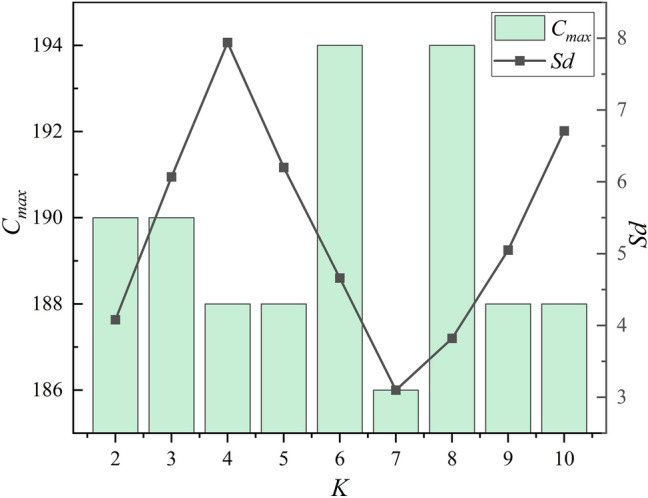
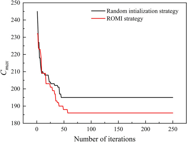
To determine the optimal value for the “K” in the ROMI, experiments are conducted using the EMK05(s) benchmark. The “K” values range from 2 to 10, resulting in nine distinct experimental setups. The results, depicted in Fig. 6, show that when “K” is set to 7, the algorithm consistently achieves lower B(C_max) and Sd values across the ten runs. Therefore, 7 is selected as the optimal parameter for the ROMI strategy. Figure 7 illustrates a detailed comparison of convergence processes for WaOA-R and WaOA, with walruses initialized by ROMI converging faster and more efficiently to a better makespan than those initialized randomly in WaOA.

Fig. 6.

Optimal selection of ROMI strategy parameter “K”.

Fig. 7.

Convergence for two initialization strategies in EMK05(s).

Table 5 presents the comparative experimental results of WaOA-R and the original WaOA across 30 test instances. The comparison reveals that incorporating the ROMI strategy improves B(C_max) in 25 instances, with 1 instance yielding identical results and only 4 instances performing worse. For Av, improvements are observed in 28 instances, with only 2 instances performing worse. Regarding the Sd metric, 22 instances show improvement, and 8 instances perform worse. These comparisons, illustrated in Table 5 and Fig. 7, suggest that WaOA-R with the ROMI strategy not only demonstrates superior search capability but also exhibits improved stability and consistency compared to WaOA, while further enhancing the algorithm’s convergence efficiency.

Table 5.

Comparison between WaOA-R and WaOA.

Instances	WaOA			WaOA-R			Instances	WaOA			WaOA-R
	B(Cmax)	Av	Sd	B(Cmax)	Av	Sd		B(Cmax)	Av	Sd	B(Cmax)	Av	Sd
EMK01(s)	47	49.1	2.4	46	48.1	1.7	EMK08(d)	550	569.4	13.7	536	558	14.7
EMK01(d)	44	47.7	3.1	42	45.6	3.1	EMK09(s)	428	447.5	12.3	423	443.1	11.1
EMK02(s)	40	45.2	2.8	33	37.5	2.1	EMK09(d)	423	458.7	16.5	415	449.3	18.2
EMK02(d)	39	42.8	2.6	36	38.4	2.2	EMK10(s)	368	384.6	15.8	355	378.2	14.2
EMK03(s)	238	258.6	9.4	236	249.8	11.2	EMK10(d)	352	395.8	16.9	357	384.9	11.3
EMK03(d)	260	274.3	6.4	231	251	10.0	EMK11(s)	675	691.2	20.4	675	689.3	17.2
EMK04(s)	82	95.3	3.9	75	80	2.9	EMK11(d)	676	689.4	17.6	654	673.4	19.8
EMK04(d)	82	92.7	4.2	78	80.8	2.1	EMK12(s)	564	598.3	23.7	553	584.5	21.2
EMK05(s)	195	203.8	5.1	186	196	3.2	EMK12(d)	579	591.3	24.8	589	599.1	20.4
EMK05(d)	202	224.6	8.5	189	197	6.7	EMK13(s)	569	625.2	40.7	558	617.4	33.5
EMK06(s)	124	148.3	7.5	112	125	7.0	EMK13(d)	576	623.8	21.6	589	633.3	24.3
EMK06(d)	122	134.5	11.7	119	130.1	8.9	EMK14(s)	758	792.3	32.8	752	788.2	28.6
EMK07(s)	173	187.4	8.5	173	185.6	8.2	EMK14(d)	773	810.2	36.2	778	806.6	31.2
EMK07(d)	194	208.7	10.4	175	189.2	10.2	EMK15(s)	567	587.5	24.1	562	584.1	25.2
EMK08(s)	566	584.1	10.5	547	568	14.8	EMK15(d)	532	581.1	27.2	521	572.8	19.8

Significant values are in bold.

Comparative experiments with enhanced WaOA variants

To validate the effectiveness and advantages of the enhanced feeding, migration, and fleeing strategies and the proposed the gathering strategy, we compare the metrics B(C_max), Av and Sd across ten runs for the algorithms WaOA-R, WaOA-RF, WaOA-RFM, WaOA-RFMF and eWaOA. The experimental results are detailed in Table 6.

Table 6.

Results obtained by different WaOA variants.

Instances	WaOA-R			WaOA-RF			WaOA-RFM			WaOA-RFMF			eWaOA
	B(Cmax)	Av	Sd	B(Cmax)	Av	Sd	B(Cmax)	Av	Sd	B(Cmax)	Av	Sd	B(Cmax)	Av	Sd
EMK01(s)	46	48.1	1.7	45	47.6	2.7	43	46.3	2.2	42	44.3	1.9	42	42.0	0.0
EMK01(d)	42	45.6	3.1	42	46.3	2.8	39	43.6	1.8	40	42.8	1.5	39	39.1	0.3
EMK02(s)	33	37.5	2.1	35	39.2	2.5	34	37.9	2.3	34	37.1	2.0	27	28.1	0.7
EMK02(d)	36	38.4	2.2	36	41.3	3.3	35	38.5	2.7	32	35.8	2.6	28	28.6	0.8
EMK03(s)	236	249.8	11.2	230	248.1	8.5	227	241	7.1	226	234.4	7.4	204	204.0	0.0
EMK03(d)	231	251	10.0	232	252.9	9.7	228	245.4	8.3	217	229.2	7.5	187	187.0	0.0
EMK04(s)	75	80	2.9	74	82.1	3.2	73	79	2.5	73	76	2.5	66	68.1	2.5
EMK04(d)	78	80.8	2.1	74	78.3	1.6	74	77.7	2.9	73	75.8	2.4	66	68.3	2.5
EMK05(s)	186	196	5.4	186	192.2	4.7	186	193.7	4.1	184	187.7	3.3	173	175.3	1.7
EMK05(d)	189	197	6.7	188	195.7	6.8	188	193.5	5.7	180	188.4	4.1	171	172.7	1.0
EMK06(s)	112	125	7.0	112	123.9	8.5	111	121.9	6.8	107	119.8	6.0	72	75.8	2.7
EMK06(d)	119	130.1	8.9	117	125.4	8.5	114	122.1	10.6	110	119.6	8.1	69	75.7	3.5
EMK07(s)	173	185.6	8.2	170	184.8	11.8	175	183.4	9.5	166	179.1	8.2	138	142.5	2.5
EMK07(d)	175	189.2	10.2	173	185.5	8.4	169	183.3	6.0	171	178.9	5.2	137	142.2	3.7
EMK08(s)	547	568	14.8	545	565.6	16.5	545	563	14.5	533	554.8	13.6	523	532.0	3.0
EMK08(d)	536	558	14.7	536	557.5	18.9	534	557.3	17.2	523	545.2	16.7	513	521.0	4.0
EMK09(s)	423	443.1	11.1	409	428.7	21.6	387	413.8	21.0	380	402.2	21.3	319	327.8	6.3
EMK09(d)	415	449.3	18.2	410	441.2	17.0	407	436.1	15.3	391	413.5	14.9	318	329.9	5.7
EMK10(s)	355	378.2	14.2	351	371.3	15.6	347	368.5	19.5	334	370.8	20.3	241	250.6	7.7
EMK10(d)	357	384.9	11.3	347	375.1	12.7	338	366.6	18.4	325	359.7	20.7	228	248.0	3.9
EMK11(s)	675	689.3	17.2	661	681.8	16.4	656	673.3	14.1	639	664.3	13.7	615	619.2	2.9
EMK11(d)	654	673.4	19.8	654	673.2	15.2	646	671.1	15.9	646	666.7	14.4	613	624.5	2.5
EMK12(s)	553	584.5	21.2	542	576	14.7	535	572	10.5	540	554.6	10.0	508	513.8	9.2
EMK12(d)	589	599.1	20.4	571	587.4	22.8	567	579.1	19.7	532	561.5	19.9	508	517.5	7.1
EMK13(s)	558	617.4	33.5	558	603	27.4	554	598.1	20.6	552	578.8	19.9	421	452.1	9.1
EMK13(d)	589	633.3	24.3	572	602.9	17.5	544	595.5	17.1	568	592.6	16.7	417	448.6	6.8
EMK14(s)	752	788.2	28.6	739	787.2	27.3	745	784.6	26.4	694	730.6	20.3	694	694.0	0.0
EMK14(d)	778	806.6	31.2	757	783.4	21.8	745	784.6	21.3	694	734.9	22.7	694	694.0	0.0
EMK15(s)	562	584.1	25.2	549	562.5	23.6	520	549.7	22.0	539	567.2	21.7	366	395.9	5.1
EMK15(d)	521	572.8	19.8	521	571.7	18.3	519	547	17.5	549	570.8	21.4	382	404.6	5.0

Significant values are in bold.

Table 6 shows that WaOA-RF surpasses WaOA-R in terms of B(C_max) for 20 out of 30 test instances, with 8 instances achieving identical results and only 2 instances showing slightly lower performance. For the Av metric, WaOA-RF demonstrates superior performance in 25 instances compared to WaOA-R, while 5 instances exhibit relatively lower Av values. Regarding the Sd metric, WaOA-RF outperforms WaOA-R in 17 instances, with 13 instances exhibiting comparatively higher Sd values. These results suggest that incorporating Lévy flight into WaOA’s feeding strategy enhances both makespan and solution stability. The key benefit of Lévy flight is its combination of short- and long-distance moves, which enables more effective exploration of the search space and better balance between exploration and exploitation.

The comparative analysis between WaOA-RFM and WaOA-RF highlights a significant performance improvement due to the enhanced migration strategy. For the B(C_max) metric, 24 test instances show notable improvement, with 2 instances experiencing a minor decline and 4 remaining unchanged. Similarly, in the Av metric, 28 test instances demonstrate performance gains, while only 2 show slight declines. Regarding the Sd metric, WaOA-RFM outperforms WaOA-RF in 25 instances, with 5 instances exhibiting relatively higher Sd values. These findings underscore the enhanced migration strategy’s effectiveness in achieving an optimal makespan, along with improved stability and consistency. This improvement is likely due to the self-adjusting factor in the migration strategy, which promotes global exploration in early iterations and strengthens local exploitation in later stages.

Comparing WaOA-RFMF with WaOA-RFM reveals that the enhanced fleeing strategy positively impacts WaOA. Specifically, for the B(C_max) metric, 21 test instances show performance gains, 6 instances experience slight declines, and 3 instances remain unchanged. In the case of the Av metric, 27 test instances show improvements, while only 3 instances perform worse than with the original fleeing strategy. For the Sd metric, 23 instances show improvements, while 7 instances perform relatively worse. These results conclusively demonstrate that the fleeing strategy with arctangent function-controlled local bounds significantly outperforms the original strategy, enhancing makespan, maintaining algorithmic consistency and stability, and reducing variability across runs.

Table 6 shows that eWaOA significantly improves the B(C_max) metric in 27 test instances compared to WaOA-RFMF, with performance in the remaining 3 instances being comparable. This result robustly demonstrates eWaOA’s potential in global optimization. Additionally, eWaOA consistently improves the Av metric across all test instances. For the Sd metric, eWaOA achieves lower values in 28 instances, with 1 instance showing the same value as WaOA-RFMF, and only 1 instance showing a minor 0.1 increase. These findings strongly indicate that the gathering strategy significantly enhances WaOA’s ability to achieve a globally optimal makespan while markedly improving stability and consistency across multiple executions and diverse test scenarios.

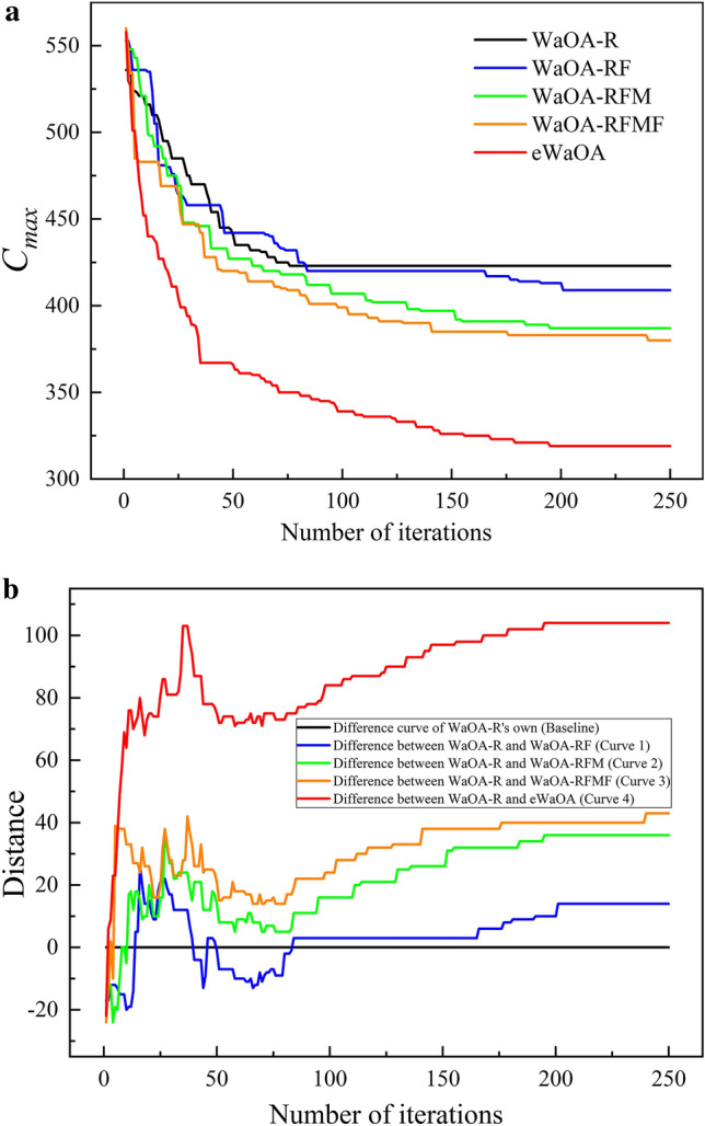
The evolutionary trajectories of these algorithms on EMK09(s) are analyzed to assess whether the refined strategies accelerate WaOA’s convergence, as illustrated in Fig. 8a. This figure demonstrates that each improvement, relative to the baseline (WaOA-R), enhances convergence speed and achieves a better makespan. As shown in Fig. 8b, Curve 1, representing the difference between WaOA-RF and WaOA-R, displays fluctuations in the early and middle iterations, suggesting that Lévy flight significantly enhances WaOA’s global exploration capabilities. In the later stages, the differences in results continue to increase until reaching stability, indicating that Lévy flight also strengthens exploitation in the middle and later iterations, allowing the algorithm to escape local optima through occasional long-distance moves.

Fig. 8.

The diversity curves for the five algorithms to solve EMK09(s).

Curve 2, representing the difference between WaOA-RFM and WaOA-RF, oscillates above the baseline with a broader range of values than Curve 1 during the early and middle stages. This pattern indicates that the enhanced migration strategy strengthens WaOA-R’s global exploration through the introduced adaptive parameter. In the middle and later stages, the differences continue to increase, reaching values significantly higher than those of Curve 1. This trend demonstrates that the adaptive parameter also facilitates more effective local search guidance.

Curve 3, which represents the difference between WaOA-RFMF and WaOA-R, shows pronounced fluctuations in the early and middle stages before transitioning into a phase of steady, stepwise improvement. Notably, Curve 3 consistently remains above Curve 2 throughout the process. This suggests that introducing the arctangent function to replace the inverse proportional function in the fleeing strategy does not diminish the global exploration capability provided by the enhanced feeding and migration strategies. Instead, it further enhances WaOA’s local search capacity in the middle and later stages. This improvement is mainly attributed to the extended global search range produced by the combined effect of the three enhanced strategies in the early and middle stages. The arctangent function expands the local bound, enabling the algorithm to perform more detailed local searches within a larger search space, thereby enhancing solution optimization in the later stages.

The combined application of all three enhanced strategies substantially improves WaOA-R's exploration and exploitation capabilities, leading to a reduced makespan. However, results indicate that WaOA still risks becoming trapped in local optima, with local search improvements progressing slowly during the middle and later stages. The proposed gathering strategy effectively addresses this issue. As shown in Fig. 8b, Curve 4, representing the difference between eWaOA and WaOA-R, remains consistently above Curve 3 throughout the process. Alongside Fig. 8a, it is clear that the algorithm demonstrates strong global search capabilities, leading to a rapid reduction in makespan and producing significantly better results than WaOA-RFMF in the early and middle stages. In the mid-to-later stages (e.g., after 75 generations), the stepwise increases in Curve 4 occur more frequently than in Curve 3, stabilizing around 200 iterations. Overall, the gathering strategy significantly enhances both exploration and exploitation in WaOA. The primary advantage of the gathering strategy lies in its random pairing of agents for positional information exchange, which prevents excessive concentration in specific regions and reduces the risk of becoming trapped in local optima. As iterations progress into the middle and later stages, shared positional information among paired agents converges, allowing individuals to refine their positions within localized areas. This process enhances both convergence speed and solution accuracy.

Figure 9 depicts the variation in the value of A according to Eq. (26) over iterations when solving EMK09(s), showing that in the early stages, the gathering strategy is highly likely to be employed, thereby enhancing WaOA’s exploration capability. Conversely, in the middle and later stages, the probability of using the gathering strategy decreases, shifting the focus toward improving exploitation. Thus, this strategy effectively balances exploration and exploitation throughout different phases. Figure 10 shows the Gantt chart for EMK09 (d), generated using the eWaOA algorithm. The chart illustrates that all operations comply with both the sequential order constraints of the process plan and the PBPO requirements. This demonstrates that the proposed methods for encoding, conversion, inverse conversion, and decoding effectively can handle the constraints of FJSP_PBPO.

Fig. 9.

The value of A over iterations of a run while solving EMK09(s).

Fig. 10.

Gantt chart of a scheduling scheme for EMK09 (d).

Comparative experiments with other metaheuristic algorithms

Due to the novelty of FJSP_PBPO, there are no publicly available algorithms for direct comparison. Meanwhile, the eWaOA proposed in this study is a standalone algorithm rather than a hybrid one. Therefore, this study selected 11 SOTA standalone metaheuristic algorithms for evaluation. Each algorithm uniformly employs the encoding scheme, conversion scheme and semi-active decoding method. The main differences among the algorithms lie in their initialization and iterative processes. These algorithms can be categorized into four groups: evolutionary-based, swarm-based, physics-based, and human-based. Evolutionary-based algorithms mimic natural evolution using selection, crossover, and mutation to optimize solutions. The GA and DE⁶⁹, renowned for their robust global search capabilities, are the most prevalent evolutionary-based algorithms. They are widely applied in scheduling optimization and are chosen as comparison algorithms for this study. Swarm-based metaheuristic algorithms are developed by modeling the collective behaviors seen in natural phenomena. This study compares classic swarm-based metaheuristic algorithms, including PSO⁴⁴ and GWO⁵¹, alongside newer algorithms such as HHO⁵⁶, artificial rabbits optimization (ARO)⁷⁰, and the latest WO¹². Physics-based algorithms utilize principles from physics to address optimization challenges. In this paper, multi-verse optimization (MVO)⁷¹ and optical microscope algorithm (OMA)⁷⁵ are chosen as comparison algorithms within the physics-based category. Human-based algorithms, inspired by human cognitive processes and behaviors, are represented here by the teaching learning based optimization (TLBO)⁷⁶ and poor and rich optimization (PRO)⁷². To eliminate variations from differences in initial candidate solutions, enhance the repeatability and stability of the experiments, and ensure fairness and consistency in evaluation, the initial population size is uniformly set to 200. Other parameters are configured according to the default settings of each algorithm, with the specific values presented in Table 7.

Table 7.

Parameter settings for the comparison algorithms.

Category	Algorithm	Parameter (value)	Category	Algorithm	Parameter (value)
Evolutionary-based	GA	Crossover rate (0.8) Mutation rate (0.05)	Swarm-based	PSO	Cognitive coefficient (2) Social coefficient (2) Inertia weight (Linear reduction from 0.9 to 0.2)
	DE	Mutation factor (0.5) Crossover probability (0.2)		GWO	Convergence parameter (Linear reduction from 2 to 0)
Physics-based	OMA	–		HHO	Escape energy (Linear reduction from 2 to 0)
	MVO	WEP_Max (1) WEP_Min (0.2)		ARO	Energy factor ([0.1, 2]) Hiding parameter ([0.01, 0.5])
Human-based	TLBO	Teaching factor (1,2)		WO	Female rate ([0.4]) Danger signal (2)
	PRO	Mutation probability (0.06)

To comprehensively evaluate the performance of the algorithms across 30 extended test instances, we conducted two experiments: one with a fixed maximum number of iterations (Experiment 1) and the other with a time-limited termination criterion, where the algorithms terminate once the time limit is reached (Experiment 2). These experiments assess each algorithm’s capability to find the global optimal solution and its trade-off between solution quality and search efficiency. We compare the metrics B(C_max), Av, Sd, RPD, SdMean, RPDMean for all 12 algorithms.

The results of Experiment 1 are presented in Table 8. Notably, eWaOA achieves optimal values for the B(C_max), Av, and PRD metrics across all 30 test instances. Specifically, eWaOA attains optimality in 26 instances for B(C_max), while in the remaining 4 instances, it ties with other top algorithms. For the Av metric, eWaOA achieves optimality in all 30 instances. Furthermore, among the 12 algorithms, eWaOA records the lowest Sd value in 22 of the test instances. In terms of SdMean and RPDMean metrics across all instances, eWaOA demonstrates superior performance with values of 3.3 and 0, respectively. Table 9 presents the termination time settings (Time) and the results of Experiment 2. As shown, eWaOA also demonstrates strong competitiveness. Specifically, eWaOA achieves the minimum values for the B(C_max), Av, and Sd metrics in 28, 30, and 15 instances, respectively. Notably, eWaOA also performs well in the SdMean and PRDMean metrics, with the lowest values of 3.9 and 0.1, respectively. These results indicate eWaOA’s efficient optimization capability within a fixed termination time.

Table 8.

Comparison results with the same maximum number of iterations.

Instance	GA				DE				PSO				GWO				HHO				ARO
	B(Cmax)	Av	Sd	RPD	B(Cmax)	Av	Sd	RPD	B(Cmax)	Av	Sd	RPD	B(Cmax)	Av	Sd	RPD	B(Cmax)	Av	Sd	RPD	B(Cmax)	Av	Sd	RPD
EMK01(s)	48	54.2	2.7	14.3	46	46.6	0.7	9.5	42	47.9	3.8	0.0	45	47.7	2.5	7.1	43	50.3	3.5	2.4	43	45.6	0.9	2.4
EMK01(d)	51	52.2	1.2	30.8	42	43.7	1.1	7.7	42	44.1	2.3	5.1	40	44.8	3.2	2.6	46	48.3	1.5	17.9	39	41.5	1.2	0.0
EMK02(s)	43	46.4	2.5	59.3	38	40.1	1.0	40.7	34	37.4	1.7	25.9	37	39.9	1.8	37.0	39	44.9	2.5	44.4	36	37.8	1.7	33.3
EMK02(d)	44	46.6	2.0	57.1	37	39.2	1.3	32.1	35	38.1	2.2	21.4	35	39.3	2.8	25.0	46	48.0	2.6	64.3	34	37.1	1.6	21.4
EMK03(s)	284	295.4	8.9	39.2	277	286.6	5.4	35.8	219	225.2	7.7	6.9	216	231.7	10.6	5.9	252	279.8	12.1	23.5	228	241.1	6.0	11.8
EMK03(d)	270	296.6	11.6	44.4	267	274.8	6.1	42.8	213	220.1	5.3	11.8	218	235.7	10.5	16.6	266	287.3	10.4	42.2	223	235.7	8.3	19.3
EMK04(s)	72	74.1	1.5	9.1	79	81.1	1.4	19.7	75	78.4	3.5	10.6	74	77.3	2.8	12.1	79	85.1	5.2	19.7	73	77.9	2.9	10.6
EMK04(d)	83	90.7	5.3	25.8	81	82.5	1.2	22.7	73	79.3	3.8	10.6	72	77.2	5.1	9.1	76	82.9	3.6	15.2	72	74.5	2.1	9.1
EMK05(s)	209	219.4	6.6	20.8	195	200.8	3.5	12.7	181	187.7	4.0	4.6	186	193.5	4.9	7.5	189	200.2	7.6	9.2	186	188.8	1.9	7.5
EMK05(d)	207	214.7	4.2	21.1	199	203.7	2.9	16.4	185	189.3	2.4	7.0	180	190.5	5.6	5.3	196	204.4	5.5	14.6	185	189.3	2.4	8.2
EMK06(s)	142	151.3	5.6	97.2	138	140.1	1.9	91.7	107	116.0	7.6	43.1	102	114.4	7.4	41.7	138	145.8	7.6	91.7	107	116.5	5.7	48.6
EMK06(d)	142	154.6	9.1	105.8	140	143.3	2.0	102.9	108	113.0	3.8	58.8	105	118.8	6.5	52.2	136	146.4	7.0	97.1	109	117.1	4.3	58.0
EMK07(s)	198	215.2	8.6	43.5	194	199.3	3.7	40.6	165	175.2	7.7	19.6	159	167.0	7.0	15.2	179	194.9	8.7	29.7	164	171.1	4.6	18.8
EMK07(d)	202	216.8	10.9	47.4	199	210.7	4.9	45.3	168	179.4	9.2	18.2	165	173.8	5.0	20.4	209	215.8	10.0	52.6	171	178.2	5.6	24.8
EMK08(s)	599	624.8	18.8	14.5	583	596.3	7.5	11.5	535	542.5	5.8	1.9	538	556.1	15.7	2.9	572	596.1	11.8	9.4	548	560.7	7.2	4.8
EMK08(d)	599	609.6	9.2	16.8	582	595.6	8.8	13.5	523	542.1	10.7	1.9	541	553.8	9.5	5.5	583	595.5	12.5	13.6	549	561.8	7.4	7.0
EMK09(s)	495	513.8	14.9	55.2	484	495.9	6.7	51.7	380	413.0	23.5	18.2	387	423.1	21.2	21.3	454	484.6	18.5	42.3	411	428.0	13.4	28.8
EMK09(d)	484	522.9	17.0	51.3	492	503.2	5.4	53.8	403	423.4	11.4	23.0	391	417.6	12.5	22.2	459	483.7	14.7	43.4	418	441.5	16.4	30.6
EMK10(s)	420	437.7	9.3	74.3	407	413.0	3.8	68.9	341	363.4	19.2	36.4	347	353.6	11.8	44.0	402	422.3	17.9	66.8	348	370.6	9.8	44.4
EMK10(d)	421	436.3	13.1	84.6	402	416.0	8.0	76.3	327	348.8	20.6	40.8	345	361.9	13.0	51.3	412	431.1	14.0	80.7	338	361.6	13.0	48.2
EMK11(s)	722	772.1	24.6	17.4	727	735.1	5.9	18.2	646	663.1	12.5	5.0	651	673.2	17.4	5.9	695	717.0	19.7	13.0	665	675.9	7.4	8.1
EMK11(d)	704	752.0	19.6	14.8	696	718.3	8.7	13.5	657	664.1	5.0	7.2	643	671.6	15.8	4.9	680	702.6	12.4	10.9	644	655.8	6.2	5.1
EMK12(s)	634	670.7	18.0	24.8	603	610.8	5.3	18.7	531	566.7	16.1	4.5	534	551.0	12.3	5.1	562	595.4	29.5	10.6	538	561.5	12.4	5.9
EMK12(d)	668	688.5	16.4	31.5	599	609.3	5.4	17.9	541	572.2	16.6	6.5	535	558.1	16.0	5.3	603	635.4	29.3	18.7	540	558.1	16.0	6.3
EMK13(s)	679	735.3	31.7	61.3	676	692.3	9.4	60.6	528	565.8	16.3	24.0	531	561.0	18.8	26.1	605	649.8	29.7	43.7	563	586.6	17.7	33.7
EMK13(d)	716	733.3	13.9	71.7	677	686.5	6.5	62.4	556	582.5	19.6	29.5	542	561.1	14.3	30.0	605	683.3	40.7	45.1	582	594.5	8.6	39.6
EMK14(s)	932	972.9	24.1	34.3	804	822.6	8.6	15.9	721	761.4	26.8	3.9	707	733.0	11.4	1.9	752	816.6	29.1	8.4	694	724.1	17.6	0.0
EMK14(d)	947	985.5	29.1	36.5	765	792.4	12.4	10.2	707	764.8	29.0	1.9	707	729.3	18.1	1.9	772	837.2	48.7	11.2	712	728.5	9.2	2.6
EMK15(s)	618	654.6	21.4	68.9	616	632.4	9.4	68.3	527	552.6	17.9	39.6	514	543.8	20.1	40.4	575	614.9	23.6	57.1	533	561.2	17.3	45.6
EMK15(d)	633	672.8	32.7	65.7	626	644.9	10.7	63.9	515	531.3	14.1	34.3	521	542.8	16.8	36.4	590	629.0	21.7	54.5	528	560.3	14.5	38.2
SdMean	13.1				5.3				11.0				10.7				15.4				8.1
RPDMean	44.6				38.2				18.8				18.8				35.1				20.8

Instance	WO				MVO				OMA				TLBO				PRO				eWaOA
	B(Cmax)	Av	Sd	RPD	B(Cmax)	Av	Sd	RPD	B(Cmax)	Av	Sd	RPD	B(Cmax)	Av	Sd	RPD	B(Cmax)	Av	Sd	RPD	B(Cmax)	Av	Sd	RPD
EMK01(s)	48	51.1	2.0	14.3	47	49.4	2.4	11.9	49	51.1	1.1	16.7	45	46.8	1.7	7.1	48	52.1	1.8	14.3	42	42.0	0.0	0.0
EMK01(d)	43	47.3	3.3	10.3	41	46.1	3.2	5.1	46	48.1	1.7	17.9	39	40.6	1.3	0.0	48	53.0	2.4	23.1	39	39.1	0.3	0.0
EMK02(s)	36	43.6	3.2	33.3	36	40.1	2.0	33.3	46	47.4	1.2	70.4	33	38.0	2.6	22.2	39	43.3	2.7	44.4	27	28.1	0.7	0.0
EMK02(d)	39	43.8	3.5	39.3	34	40.3	3.6	21.4	43	45.1	1.0	53.6	35	39.2	3.0	25.0	39	42.3	2.1	39.3	28	28.6	0.8	0.0
EMK03(s)	238	263.2	26.3	16.7	222	248.3	19.5	8.8	268	279.4	6.0	31.4	216	249.3	21.2	5.9	281	291.9	5.4	37.7	204	204.0	0.0	0.0
EMK03(d)	249	285.9	25.2	33.2	219	240.7	14.9	17.1	266	280.3	7.4	42.2	204	237.0	20.5	9.1	286	298.3	9.1	52.9	187	187.0	0.0	0.0
EMK04(s)	73	80.6	5.1	10.6	79	82.2	3.3	19.7	81	83.6	1.9	22.7	68	74.5	3.7	3.0	85	89.7	2.9	28.8	66	68.1	2.5	0.0
EMK04(d)	73	79.8	5.1	10.6	77	80.9	2.8	16.7	80	83.7	1.7	21.2	73	76.9	2.0	10.6	84	88.3	3.3	27.3	66	68.3	2.5	0.0
EMK05(s)	190	200.2	7.6	9.8	188	198.0	7.8	8.7	203	207.2	3.1	17.3	186	195.7	6.3	7.5	213	223.8	4.6	23.1	173	175.3	1.7	0.0
EMK05(d)	180	192.7	5.6	5.3	191	197.6	6.1	11.7	202	204.0	1.5	18.1	175	189.1	6.6	2.3	213	221.1	5.3	24.6	171	172.7	1.0	0.0
EMK06(s)	119	138.9	18.0	65.3	115	127.2	7.4	59.7	142	147.3	3.4	97.2	113	127.4	9.0	56.9	153	160.7	5.5	112.5	72	75.8	2.7	0.0
EMK06(d)	111	139.5	14.5	60.9	114	127.6	9.3	65.2	141	147.9	3.7	104.3	107	126.1	12.1	55.1	146	156.1	6.5	111.6	69	75.7	3.5	0.0
EMK07(s)	176	201.2	13.4	27.5	172	185.8	7.3	24.6	191	200.4	4.8	38.4	164	179.5	11.4	18.8	204	214.8	7.5	47.8	138	142.5	2.5	0.0
EMK07(d)	182	201.8	12.8	32.8	179	189.6	11.5	30.7	206	209.3	4.6	50.4	156	171.1	9.2	13.9	201	214.1	8.4	46.7	137	142.2	3.7	0.0
EMK08(s)	548	582.2	30.2	4.8	553	573.9	17.5	5.7	582	590.3	4.5	11.3	563	581.6	10.9	7.6	604	613.4	8.2	15.5	523	532.0	3.0	0.0
EMK08(d)	526	586.6	45.3	2.5	552	576.5	21.4	7.6	573	584.8	6.7	11.7	535	574.4	17.9	4.3	599	634.6	15.6	16.8	513	521.0	4.0	0.0
EMK09(s)	423	483.9	32.3	32.6	413	439.2	14.0	29.5	493	503.2	6.1	54.5	439	462.1	17.2	37.6	481	523.3	20.9	50.8	319	327.8	6.3	0.0
EMK09(d)	485	495.3	28.9	51.6	418	441.1	15.6	30.6	500	505.9	4.0	56.3	396	443.3	39.2	23.8	503	538.8	17.9	57.2	318	329.9	5.7	0.0
EMK10(s)	357	414.3	41.4	48.1	345	375.5	20.2	43.2	417	429.3	7.7	73.0	383	421.3	15.4	58.9	436	453.0	11.9	80.9	241	250.6	7.7	0.0
EMK10(d)	378	417.7	41.4	65.8	344	372.3	15.0	50.9	434	443.0	7.1	90.4	368	410.0	24.3	61.4	430	454.4	15.3	88.6	228	248.0	3.9	0.0
EMK11(s)	677	702.1	24.3	10.1	666	686.7	14.9	8.3	691	708.2	8.4	12.4	682	695.9	10.4	10.9	714	738.5	16.4	16.1	615	619.2	2.9	0.0
EMK11(d)	683	717.7	33.2	11.4	670	682.3	10.6	9.3	714	726.5	6.9	16.5	695	718.6	15.4	13.4	723	757.7	14.5	17.9	613	624.5	2.5	0.0
EMK12(s)	552	605.0	36.2	8.7	573	591.7	15.1	12.8	572	581.2	5.6	12.6	529	549.7	13.6	4.1	639	655.4	9.8	25.8	508	513.8	9.2	0.0
EMK12(d)	564	589.0	34.0	11.0	540	584.0	28.7	6.3	572	596.4	11.1	12.6	533	558.1	17.6	4.9	617	654.7	18.6	21.5	508	517.5	7.1	0.0
EMK13(s)	605	665.3	49.9	43.7	564	612.2	33.7	34.0	687	716.9	13.3	63.2	541	635.0	50.3	28.5	711	745.6	23.1	68.9	421	452.1	9.1	0.0
EMK13(d)	552	668.0	74.3	32.4	566	612.6	30.8	35.7	718	727.1	5.6	72.2	493	607.3	54.2	18.2	680	725.6	30.3	63.1	417	448.6	6.8	0.0
EMK14(s)	727	756.1	22.4	4.8	727	782.4	41.5	4.8	734	757.1	14.1	5.8	694	716.2	10.2	0.0	882	915.0	25.5	27.1	694	694.0	0.0	0.0
EMK14(d)	733	779.0	38.2	5.6	759	808.7	22.9	9.4	748	767.6	15.8	7.8	694	705.1	11.8	0.0	873	926.2	35.8	25.8	694	694.0	0.0	0.0
EMK15(s)	541	628.1	46.0	47.8	517	565.8	29.0	41.3	621	643.2	10.7	69.7	630	650.8	13.2	72.1	648	673.8	16.1	77.0	366	395.9	5.1	0.0
EMK15(d)	548	611.8	58.6	43.5	535	573.9	32.1	40.1	640	657.1	7.8	67.5	548	620.7	31.2	43.5	673	688.9	11.3	76.2	382	404.6	5.0	0.0
sdMean	26.1				15.5				5.9				15.4				12.0				3.3
RPDMean	26.5				23.5				41.3				20.9				45.4				0.0

Significant values are in bold.

Table 9.

Comparison results with identical time-limited termination.

Instance	Time (s)	GA				DE				PSO				GWO				HHO				ARO
		B(Cmax)	Av	Sd	RPD	B(Cmax)	Av	Sd	RPD	B(Cmax)	Av	Sd	RPD	B(Cmax)	Av	Sd	RPD	B(Cmax)	Av	Sd	RPD	B(Cmax)	Av	Sd	RPD
EMK01(s)	60	49	53.6	3.1	16.7	43	44.3	0.8	2.4	43	47.9	2.4	2.4	44	46.5	1.8	4.8	46	48.8	2.0	9.5	42	44.7	1.9	0.0
EMK01(d)	60	48	51.8	2.9	23.1	40	41.5	0.8	2.6	41	43.9	2.2	5.1	41	44.4	2.6	5.1	41	46.4	3.1	5.1	39	39.7	0.9	0.0
EMK02(s)	60	40	44.3	2.4	42.9	36	38.1	0.9	28.6	35	36.3	1.1	25.0	37	40.0	2.1	32.1	38	41.6	2.1	35.7	34	36.6	1.9	21.4
EMK02(d)	60	43	44.9	1.8	53.6	36	38.1	1.2	28.6	34	35.9	1.6	21.4	36	39.2	2.2	28.6	41	44.5	2.5	46.4	33	35.5	1.4	17.9
EMK03(s)	120	272	285.4	8.7	33.3	264	271.6	4.1	29.4	206	215.0	6.8	1.0	214	229.5	8.7	4.9	256	273.4	7.9	25.5	219	223.8	5.2	7.4
EMK03(d)	120	262	279.3	10.6	40.1	265	271.2	3.9	41.7	203	221.2	10.6	8.6	204	228.9	15.3	9.1	249	270.7	13.0	33.2	208	218.3	6.8	11.2
EMK04(s)	120	82	89.1	3.3	22.4	75	77.6	1.6	11.9	73	75.3	2.2	9.0	73	78.2	3.3	9.0	76	83.0	5.5	13.4	72	73.7	1.3	7.5
EMK04(d)	120	85	90.5	4.2	28.8	75	78.2	1.8	13.6	73	76.2	3.2	10.6	73	76.2	2.6	10.6	75	83.0	4.9	13.6	70	72.8	1.4	6.1
EMK05(s)	60	204	214.9	7.6	17.2	193	199.2	2.4	10.9	180	185.9	3.1	3.4	187	191.1	2.8	7.5	193	202.6	7.7	10.9	179	183.8	3.4	2.9
EMK05(d)	60	204	215.1	5.9	18.6	194	199.1	2.6	12.8	181	186.1	4.2	5.2	179	191.1	5.2	4.1	195	204.8	7.5	13.4	180	184.9	3.6	4.7
EMK06(s)	150	132	143.9	5.9	78.4	130	134.3	2.9	75.7	100	109.5	4.7	35.1	103	109.7	4.3	39.2	131	142.6	8.2	77.0	100	105.6	2.7	35.1
EMK06(d)	150	134	151.2	9.9	71.8	134	137.4	2.4	71.8	101	109.3	5.4	29.5	103	111.5	7.1	32.1	127	139.7	7.8	62.8	95	107.7	4.6	21.8
EMK07(s)	100	197	212.7	6.7	36.8	183	190.0	3.8	27.1	155	163.8	5.5	7.6	163	167.2	3.7	13.2	181	193.4	7.4	25.7	159	165.7	4.9	10.4
EMK07(d)	100	204	220.0	10.3	39.7	190	194.0	2.3	30.1	161	167.8	4.8	10.3	158	171.6	7.7	8.2	181	198.3	10.9	24.0	159	165.6	6.4	8.9
EMK08(s)	200	596	614.8	19.0	12.5	580	586.5	5.2	9.4	530	546.4	8.8	0.0	533	550.8	12.1	0.6	545	577.5	15.4	2.8	533	535.4	3.3	0.6
EMK08(d)	200	580	613.4	18.3	13.1	562	579.8	9.1	9.6	523	541.8	11.5	1.9	524	547.4	20.4	2.1	557	576.9	15.2	8.6	523	528.1	5.0	1.9
EMK09(s)	200	478	511.4	22.1	48.4	459	476.4	7.7	42.5	368	390.8	15.3	14.3	400	415.1	12.8	24.2	440	475.2	20.4	36.6	387	401.0	13.1	20.2
EMK09(d)	200	480	509.4	21.4	48.1	464	476.5	5.3	43.2	381	397.0	10.6	17.6	397	416.4	9.7	22.5	446	467.8	15.9	37.7	358	395.5	15.2	10.5
EMK10(s)	300	403	427.8	16.5	60.6	394	403.6	6.2	57.0	318	332.6	10.2	26.7	333	350.9	13.3	32.7	391	404.4	11.3	55.8	326	339.3	10.0	29.9
EMK10(d)	300	408	436.5	15.9	62.5	390	405.3	7.5	55.4	316	333.2	10.4	25.9	324	346.8	14.9	29.1	382	408.7	12.7	52.2	319	334.2	9.6	27.1
EMK11(s)	150	721	755.4	23.2	16.9	702	710.0	5.5	13.8	641	655.5	8.6	3.9	642	657.2	10.7	4.1	678	706.5	19.5	9.9	636	649.6	7.9	3.1
EMK11(d)	150	717	757.5	25.8	16.2	692	705.6	6.8	12.2	645	658.4	10.2	4.5	644	656.9	8.7	4.4	675	702.2	17.1	9.4	641	647.2	5.7	3.9
EMK12(s)	300	610	659.8	27.0	20.1	577	583.0	4.3	13.6	524	558.8	16.3	3.1	524	550.2	16.0	3.1	572	599.2	16.4	12.6	531	544.6	10.0	4.5
EMK12(d)	300	627	672.1	20.4	23.4	576	588.1	7.0	13.4	524	552.0	17.3	3.1	534	550.4	12.0	5.1	564	597.8	29.7	11.0	524	550.4	12.0	3.1
EMK13(s)	300	698	738.9	17.8	53.4	624	654.0	15.8	37.1	511	542.4	24.5	12.3	529	552.3	15.7	16.3	608	644.7	28.6	33.6	512	543.4	13.0	12.5
EMK13(d)	300	696	732.1	20.8	56.8	646	660.5	7.0	45.5	501	534.5	16.5	12.8	535	560.2	14.9	20.5	586	652.9	32.0	32.0	528	543.8	14.4	18.9
EMK14(s)	450	895	963.3	38.0	29.0	750	771.9	12.3	8.1	694	738.2	38.4	0.0	694	730.5	16.8	0.0	745	789.0	32.0	7.3	694	723.1	16.0	0.0
EMK14(d)	450	929	963.8	29.7	33.9	747	771.7	10.5	7.6	714	757.5	27.9	2.9	694	724.8	18.5	0.0	720	802.2	36.4	3.7	694	700.6	11.1	0.0
EMK15(s)	450	644	664.0	14.2	63.9	608	620.4	8.8	54.7	473	498.9	12.9	20.4	498	525.0	15.2	26.7	571	612.3	27.0	45.3	486	507.4	15.7	23.7
EMK15(d)	450	625	656.4	25.9	56.6	583	623.4	16.9	46.1	494	515.8	17.8	23.8	511	537.5	14.1	28.1	576	628.1	26.4	44.4	494	511.2	14.7	23.8
SdMean		14.6				5.6				10.5				9.8				14.9				9.8
RPDMean		38.0				28.5				11.6				14.3				26.6				14.3

Instance	Time (s)	WO				MVO				OMA				TLBO				PRO				eWaOA
		B(Cmax)	Av	Sd	RPD	B(Cmax)	Av	Sd	RPD	B(Cmax)	Av	Sd	RPD	B(Cmax)	Av	Sd	RPD	B(Cmax)	Av	Sd	RPD	B(Cmax)	Av	Sd	RPD
EMK01(s)	60	45	49.3	2.8	7.1	46	48.0	2.4	9.5	46	49.6	1.4	9.5	42	44.7	3.0	0.0	48	52.1	1.8	14.3	42	42.0	0.0	0.0
EMK01(d)	60	42	46.4	3.0	7.7	42	46.7	2.6	7.7	44	47.1	1.4	12.8	39	40.6	1.3	0.0	48	53.0	2.4	23.1	39	39.4	0.9	0.0
EMK02(s)	60	34	41.7	4.0	21.4	37	40.5	2.4	32.1	43	44.3	0.6	53.6	33	36.4	2.1	17.9	39	43.3	2.7	39.3	28	29.0	0.4	0.0
EMK02(d)	60	37	38.9	2.1	32.1	35	38.2	2.4	25.0	42	44.2	1.3	50.0	33	36.0	2.0	17.9	39	42.3	2.1	39.3	28	29.3	1.1	0.0
EMK03(s)	120	223	250.5	21.2	9.3	220	239.2	15.0	7.8	264	275.6	5.1	29.4	204	224.5	15.5	0.0	281	291.9	5.4	37.7	204	204.0	0.0	0.0
EMK03(d)	120	217	253.7	20.1	16.0	214	233.5	9.5	14.4	263	273.3	6.1	40.6	194	213.1	22.4	3.7	279	291.6	9.2	49.2	187	188.2	3.6	0.0
EMK04(s)	120	73	76.6	3.9	9.0	74	80.8	4.9	10.4	80	81.4	1.4	19.4	67	72.2	2.4	0.0	85	89.8	2.9	26.9	67	69.0	2.8	0.0
EMK04(d)	120	73	81.3	5.9	10.6	73	81.2	3.8	10.6	79	80.4	1.1	19.7	66	70.6	2.9	0.0	83	87.3	3.3	25.8	67	70.5	3.1	1.5
EMK05(s)	60	183	195.1	10.0	5.2	193	199.3	6.2	10.9	195	198.6	2.6	12.1	179	186.5	5.4	2.9	206	216.9	4.5	18.4	174	175.9	1.3	0.0
EMK05(d)	60	185	198.0	7.9	7.6	188	194.3	5.7	9.3	190	196.8	3.5	10.5	176	180.7	2.8	2.3	207	214.4	5.1	20.3	172	176.5	2.3	0.0
EMK06(s)	150	110	124.5	11.2	48.6	112	123.9	5.9	51.4	137	145.4	3.5	85.1	94	109.3	13.0	27.0	146	154.4	5.1	97.3	74	79.8	4.1	0.0
EMK06(d)	150	114	128.8	14.8	46.2	109	122.8	8.4	39.7	145	147.1	2.7	85.9	93	101.8	7.1	19.2	144	154.7	6.1	84.6	78	81.9	4.0	0.0
EMK07(s)	100	174	183.4	8.8	20.8	167	187.5	10.5	16.0	188	194.5	3.1	30.6	148	158.0	7.3	2.8	202	212.8	7.5	40.3	144	150.0	3.9	0.0
EMK07(d)	100	166	192.1	25.3	13.7	159	178.5	10.5	8.9	185	196.6	4.6	26.7	148	155.5	5.2	1.4	205	214.4	6.8	40.4	146	152.2	4.2	0.0
EMK08(s)	200	533	555.1	20.1	0.6	544	572.7	16.9	2.6	559	580.5	9.6	5.5	533	556.2	13.5	0.6	604	613.4	8.2	14.0	533	533.0	0.0	0.6
EMK08(d)	200	540	560.9	25.2	5.3	528	569.1	27.2	2.9	562	581.1	9.4	9.6	524	540.8	12.6	2.1	585	617.6	14.1	14.0	513	522.0	3.0	0.0
EMK09(s)	200	399	466.3	49.8	23.9	419	436.7	16.3	30.1	482	493.6	6.2	49.7	365	406.8	29.3	13.4	481	522.2	20.9	49.4	322	334.9	8.5	0.0
EMK09(d)	200	393	435.9	31.9	21.3	417	435.4	10.3	28.7	476	496.2	8.3	46.9	370	407.1	35.8	14.2	518	530.2	12.4	59.9	324	334.3	6.9	0.0
EMK10(s)	300	341	400.2	46.2	35.9	342	358.3	11.8	36.3	416	423.2	4.4	65.7	311	386.0	28.1	23.9	432	449.0	11.9	72.1	251	263.4	8.0	0.0
EMK10(d)	300	337	393.9	41.7	34.3	339	363.5	13.2	35.1	418	425.7	4.2	66.5	299	355.8	37.8	19.1	428	453.2	11.3	70.5	251	260.4	5.8	0.0
EMK11(s)	150	651	689.5	33.4	5.5	656	688.2	21.5	6.3	695	700.7	3.5	12.6	633	659.0	18.6	2.6	736	756.9	13.1	19.3	617	624.9	4.2	0.0
EMK11(d)	150	643	680.0	29.1	4.2	664	685.3	12.3	7.6	689	703.4	6.5	11.7	622	651.8	20.3	0.8	730	752.3	15.5	18.3	617	623.4	4.4	0.0
EMK12(s)	300	524	553.1	16.1	3.1	550	593.3	32.5	8.3	540	549.0	7.2	6.3	513	532.3	10.4	1.0	609	640.3	17.8	19.9	508	521.8	7.5	0.0
EMK12(d)	300	540	573.2	27.7	6.3	562	581.8	19.9	10.6	566	582.7	9.6	11.4	524	532.2	10.3	3.1	630	669.4	21.4	24.0	508	520.2	8.5	0.0
EMK13(s)	300	592	661.4	51.7	30.1	558	589.3	22.6	22.6	661	677.9	12.5	45.3	507	553.9	43.0	11.4	666	717.0	26.3	46.4	455	460.6	4.2	0.0
EMK13(d)	300	558	623.0	53.8	25.7	558	599.4	28.6	25.7	668	692.9	11.5	50.5	467	547.6	48.8	5.2	685	716.3	18.5	54.3	444	456.5	6.0	0.0
EMK14(s)	450	707	733.0	22.7	1.9	752	789.1	21.0	8.4	707	734.6	15.3	1.9	707	718.5	8.2	1.9	868	915.6	23.7	25.1	694	694.0	0.0	0.0
EMK14(d)	450	694	710.3	16.9	0.0	772	803.4	23.9	11.2	712	735.7	14.3	2.6	694	703.6	12.6	0.0	850	896.0	36.3	22.5	694	694.0	0.0	0.0
EMK15(s)	450	550	610.9	44.2	39.9	521	554.9	22.0	32.6	612	636.5	11.7	55.7	462	586.1	51.2	17.6	648	676.2	16.1	64.9	393	402.3	7.6	0.0
EMK15(d)	450	541	605.6	39.4	35.6	528	561.7	24.1	32.3	631	645.0	8.5	58.1	471	547.9	54.6	18.0	650	682.5	19.9	62.9	399	415.3	9.8	0.0
SdMean		23.0				13.8				6.0				17.6				11.7				3.9
RPDMean		17.6				18.5				32.9				7.7				39.8				0.1

Significant values are in bold.

For each algorithm, we select the iteration data with the minimum C_max from 10 runs and then plot the C_max variation curves for different test instances, as shown in Fig. 11. In this figure, eWaOA attains the lowest C_max in all 30 instances. Moreover, the eWaOA achieves better C_max values with significantly fewer iterations (less than 50) for instances like EMK01(s), EMK01(d), EMK03(s), EMK04(s), EMK04(d), EMK05(s), EMK08(s), EMK08(d), EMK14(s), and EMK14(d). For instances EMK03(d), EMK05(d), EMK07(s), EMK11(d), EMK12(s), and EMK12(d), the convergence curve of eWaOA stabilizes within 50–100 iterations. For instances EMK02(s), EMK07(d), EMK09(s), EMK09(d), EMK13(d), EMK15(s), and EMK15(d), convergence stability is achieved within 100–200 iterations. For instances EMK02(d), EMK06(s), EMK06(d), EMK10(d), EMK11(s), and EMK13(s), stability is achieved before 250 iterations.

Fig. 11.

Iterative results of various algorithms for solving FJSP_PBPO instances.

To highlight the remarkable advantages of eWaOA over other algorithms, a paired t-test was conducted at a significance level of α = 0.05 to explore the existence of statistically significant differences between eWaOA and various comparative algorithms. The data for this paired t-test were obtained from the outcomes of running eWaOA and each comparative algorithm 10 times per instance. Figure 12 shows the results of the paired t-test regarding the C_max of eWaOA and comparative algorithms for each test instance. In this figure, each group on the x-axis represents the paired t-test results of eWaOA against a specific comparative algorithm, and the log2FC shown is calculated based on the average values of C_max. Specifically, we first determine the fold change of the average C_max of eWaOA compared to that of each comparative algorithm and then take the logarithm to the base 2 of this fold change. Moreover, according to the p-values from the paired t-test, the scatter points in the graph are divided into two groups: the group with a “p-value ≤ 0.05” is represented by red scatter points, indicating a statistically significant difference, while the group with a “p-value > 0.05” is shown by blue scatter points. To avoid complete horizontal overlap of data points and improve the readability of the scatter plot, random perturbations have been applied to each data point during the plotting process. As can be seen from the figure, except for the EMK14(d) instance in the comparison between eWaOA and ARO, and the EMK07(d) instance in the comparison between eWaOA and TLBO, eWaOA shows highly significant differences from other algorithms in most instances, as demonstrated by the distribution of red and blue scatter points as well as the values of log2FC.

Fig. 12.

The results of the paired t -test between eWaOA and the other 11 SOTA algorithms for the 30 test instances.

Based on the results in Tables 8 and 9, as well as Figd. 11 and 12, we conclude that the proposed eWaOA significantly outperforms the 11 SOTA algorithms in both optimization effectiveness and efficiency. Specifically, eWaOA demonstrates superior performance in terms of makespan, stability, consistency, and optimization efficiency-achieving better results within the specified time.

Engineering case study

This study aims to further validate the proposed eWaOA by applying it to a practical engineering scenario involving three distinct product categories tested at an electronic product performance lab. The products include mobile phones (MP), in-vehicle navigators (IVNs), and unmanned aerial vehicles (UAVs). The performance testing process plan for MP is illustrated in Fig. 1, while the testing process plan for IVNs and UAVs are detailed in Tables 10 and 11, respectively.

Table 10.

Process plan of the IVNs.

Tasks of IVN	Machine	Processing time	Tasks of IVN	Machine	Processing time
O11 (Electrical performance test)	M4	10	O42(High temperature functional test)	M3	13
O12 (Button operation force test)	M7	12	O43 (Low temperature exposure test)	M6	17
O21 (Dimensional inspection)	M2	14	O44 (Low temperature functional test)	M8	17
O22 (Rapid thermal cycling test)	M3	19	O45 (Humidity and temperature cycling Test)	M7	19
O23 (Key operation durability test)	M4	13	{O37, O46}(Dust test)	M1	15
{O13, O24}(Drop impact test)	M3	18	O51 (Appearance function test)	M5/ M8	15/15
O31 (Static current test)	M1	12	O61 (Conductive emission test)	M7	17
O32 (Operating voltage range test)	M1	15	O62 (Radiated emission test)	M8	18
O33 (Alcohol screening)	M2	17	O63 (Radiated immunity test)	M3	15
O34 (Fuel injector adhesion point inspection)	M5	17	O64 (Electrostatic discharge test)	M3	16
O35 (Artificial sweat test)	M6	19	O65 (Temperature cycling test)	M6	16
O36 (Swabbing test)	M2	12	O71 (Lifetime testing)	M5/M8	16/16
O41(High temperature exposure test)	M4	15

Table 11.

Process plan of the UAVs.

Tasks of IVN	Machine	Processing time	Tasks of UAVs	Machine	Processing time
O11 (High-low temperature charge–discharge test)	M1	17	O31 (Key/Button test)	M4	18
O12 (High-low temperature flight test)	M8	14	O32 (Transportation vibration Test)	M6	17
O13 (Swelling rainfall test)	M4	15	O33 (Handling Test)	M2	19
O21 (Corrosion resistance test)	M2	10	O34 (Circuit bending test)	M5/M8	12/12
O22 (Maximum load aging test)	M5	19	O41(Battery insertion and removal test)	M2	14
O23 (Spraying aging test)	M3	16	O42(Six-sided drop test)	M7	12
{O14, O24}(drop impact test)	M2	10	O43 (Dustproof test)	M1	17
			O44 (Immersion water test)	M6	15

The results obtained by applying the 12 algorithms to the engineering case are presented in Table 12. All algorithms use an time-limited termination criterion, with the corresponding time limit set to 55(s). It is evident that PSO, GWO, ARO, TLBO, and eWaOA yield the smallest B(C_max), with eWaOA achieving the lowest Av and Sd. This further demonstrates that eWaOA not only minimizes B(C_max) but also shows superior stability and consistency. Figure 13 displays the Gantt chart of the optimal scheduling results from 10 runs of eWaOA, with PBPOs highlighted in red boxes. The chart demonstrates that all operations adhere to the sequential order constraints of the process plan and satisfy the PBPO requirements, reaffirming the feasibility and effectiveness of eWaOA in solving the FJSP_PBPO.

Table 12.

Comparison of scheduling results for instance from testing workshop.

GA			DE			PSO			GWO
B(Cmax)	Av	Sd	B(Cmax)	Av	Sd	B(Cmax)	Av	Sd	B(Cmax)	Av	Sd
135	144.7	5.59	129	129.5	0.81	128	130.6	4.13	128	129.2	0.75

HHO			ARO			WO			MVO
B(Cmax)	Av	Sd	B(Cmax)	Av	Sd	B(Cmax)	Av	Sd	B(Cmax)	Av	Sd
129	133.0	5.50	128	128.8	0.60	129	131.2	2.79	129	132.3	2.65

OMA			TLBO			PRO			eWaOA
B(Cmax)	Av	Sd	B(Cmax)	Av	Sd	B(Cmax)	Av	Sd	B(Cmax)	Av	Sd
129	128.9	0.30	128	128.7	0.46	130	137.0	5.23	128	128.1	0.30

Significant values are in bold.

Fig. 13.

Gantt chart of a scheduling scheme obtained by eWaOA for the practical example.

Conclusion and future research

To optimize the makespan for the FJSP_PBPO problem, this study develops an optimization model using MIP and introduces an enhanced swarm-based metaheuristic algorithm, eWaOA, which extends the WaOA framework. In eWaOA, new schemes for encoding, conversion, inverse conversion, and decoding tailored to the specific constraints of FJSP_PBPO are designed. Additionally, a ROMI strategy is designed to generate diverse and high-quality initial solutions. Enhancements are made to the feeding, migration, and fleeing strategies of WaOA, and a novel gathering strategy is introduced to improve both exploration and exploitation.

To evaluate these improvements, 30 test instance, extended from existing benchmark FJSP instances, are used. The ROMI initialization strategy shows superior search capability, stability, and consistency compared to WaOA, enhancing convergence efficiency. Comparisons are made with four enhanced WaOA variants and eleven SOTA metaheuristic algorithms on the 30 test instances, followed by a real-world engineering case study. Results from these comparisons confirm that the eWaOA effectively addresses the FJSP_PBPO, demonstrating superior optimization capability, stability, consistency, and efficiency.

The proposed eWaOA primarily addresses the FJSP with PBPO. However, electronic product performance testing introduces additional constraints, including multi-resource coupling and sequence-dependent setup times. Future research will focus on enhancing eWaOA to effectively handle these constraints, extending its applicability to more complex engineering scenarios.

Author contributions

Shengping Lv: Conducted investigation, led conceptualization, managed data curation, performed formal analysis, established methodology, provided resources, was responsible for writing the original draft, carried out writing-review & editing, and oversaw project administration. Jianwei Zhuang: Handled data curation, executed formal analysis, developed methodology, worked on software, ensured validation, contributed to visualization, and participated in writing the original draft and writing-review & editing. Zhuohui Li: Managed data curation, carried out formal analysis, devised methodology, worked with software, achieved validation, and assisted with visualization. Hucheng Zhang: Took care of data curation, conducted formal analysis, formulated methodology, used software, attained validation, and helped with visualization. Hong Jin: Performed investigation, contributed to conceptualization, carried out formal analysis, and engaged in review & editing. Shengxiang Lü: Participated in conceptualization, developed methodology, and was involved in writing-review & editing.

Data availability

The authors confirm that the data supporting the findings of this study are available within the paper.

Declarations

Competing interests

The authors declare no competing interests.

References

- 1.Brucker, P. & Schlie, R. Job-shop scheduling with multi-purpose machines. Computing45, 369–375. 10.1007/BF02238804 (1990). [Google Scholar]
- 2.Brandimarte, P. Routing and scheduling in a flexible job shop by tabu search. Ann. Oper. Res.41, 157–183. 10.1007/BF02023073 (1993). [Google Scholar]
- 3.Xie, J., Gao, L., Peng, K. K., Li, X. Y. & Li, H. R. Review on flexible job shop scheduling. IET Coll. Intell. Manuf.1, 67–77. 10.1049/iet-cim.2018.0009 (2019). [Google Scholar]
- 4.Dauzère-Pérès, S., Ding, J. W., Shen, L. J. & Tamssaouet, K. The flexible job shop scheduling problem: A review. Eur. J. Oper. Res.314, 409–432. 10.1016/j.ejor.2023.05.017 (2024). [Google Scholar]
- 5.Fowler, J. W. & Mönch, L. A survey of scheduling with parallel batch (p-batch) processing. Eur. J. Oper. Res.298, 1–24. 10.1016/j.ejor.2021.06.012 (2022). [Google Scholar]
- 6.Luo, S., Zhang, L. X. & Fan, Y. S. Energy-efficient scheduling for multi-objective flexible job shops with variable processing speeds by grey wolf optimization. J. Clean. Prod.234, 1365–1384. 10.1016/j.jclepro.2019.06.151 (2019). [Google Scholar]
- 7.Liu, M., Yao, X. F. & Li, Y. X. Hybrid whale optimization algorithm enhanced with Lévy flight and differential evolution for job shop scheduling problems. Appl. Soft Comput.87, 105954. 10.1016/j.asoc.2019.105954 (2020). [Google Scholar]
- 8.Ye, S. & Bu, T. M. A self-learning Harris hawks optimization algorithm for flexible job shop scheduling with setup times and resource constraints. In 2021 IEEE Int. Conf. Syst., Man, Cybern. (SMC) 2642–2649. 10.1109/SMC52423.2021.9659113 (2021).
- 9.Yang, Z., Liang, X., Li, Y. & Wang, H. A hybrid remora optimization algorithm with variable neighborhood search for the flexible job shop scheduling problem. In 2024 7th Int. Conf. Adv. Algorithms Control Eng. (ICAACE) 942–950. 10.1109/ICAACE61206.2024.10548408 (2024).
- 10.Lv, Z. L., Zhao, Y. X., Kang, H. Y., Gao, Z. Y. & Qin, Y. H. An improved Harris Hawk optimization algorithm for flexible job shop scheduling problem. Comput. Mater. Concr.78, 2337–2360. 10.32604/cmc.2023.045826 (2024). [Google Scholar]
- 11.Wolpert, D. H. & Macready, W. G. No free lunch theorems for optimization. IEEE Trans. Evol. Comput.1, 67–82. 10.1109/4235.585893 (1997). [Google Scholar]
- 12.Han, M. et al. Walrus optimizer: A novel nature-inspired metaheuristic algorithm. Expert Syst. Appl.239, 122413. 10.1016/j.eswa.2023.122413 (2024). [Google Scholar]
- 13.Fontes, D. B. M. M., Homayouni, S. M. & Gonçalves, J. F. A hybrid particle swarm optimization and simulated annealing algorithm for the job shop scheduling problem with transport resources. Eur. J. Oper. Res.306, 1140–1157. 10.1016/j.ejor.2022.09.006 (2023). [Google Scholar]
- 14.Zhang, F., Li, R. & Gong, W. Deep reinforcement learning-based memetic algorithm for energy-aware flexible job shop scheduling with multi-AGV. Comput. Ind. Eng.189, 109917. 10.1016/j.cie.2024.109917 (2024). [Google Scholar]
- 15.Chen, X., Li, J., Wang, Z., Li, J. & Gao, K. A genetic programming based cooperative evolutionary algorithm for flexible job shop with crane transportation and setup times. Appl. Soft Comput.169, 112614. 10.1016/j.asoc.2024.112614 (2025). [Google Scholar]
- 16.Li, J., Han, Y., Gao, K., Xiao, X. & Duan, P. Bi-population balancing multi-objective algorithm for fuzzy flexible job shop with energy and transportation. IEEE Trans. Autom. Sci. Eng.21, 4686–4702. 10.1109/TASE.2023.3300922 (2024). [Google Scholar]
- 17.Hu, C., Zheng, R., Lu, S., Liu, X. & Cheng, H. Integrated optimization of production scheduling and maintenance planning with dynamic job arrivals and mold constraints. Comput. Ind. Eng.186, 109708. 10.1016/j.cie.2023.109708 (2023). [Google Scholar]
- 18.Meng, L., Zhang, C., Zhang, B. & Ren, Y. Mathematical modeling and optimization of energy-conscious flexible job shop scheduling problem with worker flexibility. IEEE Access7, 68043–68059. 10.1109/ACCESS.2019.2916468 (2019). [Google Scholar]
- 19.Zhang, S. et al. Dual resource constrained flexible job shop scheduling based on improved quantum genetic algorithm. Machines9, 108. 10.3390/machines9060108 (2021). [Google Scholar]
- 20.Zhang, H., Xu, G., Pan, R. & Ge, H. A novel heuristic method for the energy-efficient flexible job-shop scheduling problem with sequence-dependent set-up and transportation time. Eng. Optim.54, 1646–1667. 10.1080/0305215X.2021.1949007 (2022). [Google Scholar]
- 21.Gao, K. Z. et al. An improved artificial bee colony algorithm for flexible job-shop scheduling problem with fuzzy processing time. Expert Syst. Appl.65, 52–67. 10.1016/j.eswa.2016.07.046 (2016). [Google Scholar]
- 22.Chen, N., Xie, N. & Wang, Y. An elite genetic algorithm for flexible job shop scheduling problem with extracted grey processing time. Appl. Soft Comput.131, 109783. 10.1016/j.asoc.2022.109783 (2022). [Google Scholar]
- 23.Graham, R. L., Lawler, E. L., Lenstra, J. K. & Kan, A. H. G. R. Optimization and approximation in deterministic sequencing and scheduling: A survey. Ann. Discret. Math.5, 287–326. 10.1016/S0167-5060(08)70356-X (1979). [Google Scholar]
- 24.Adams, J., Balas, E. & Zawack, D. The shifting bottleneck procedure for job shop scheduling. Manag. Sci.34, 391–401. 10.1287/mnsc.34.3.391 (1988). [Google Scholar]
- 25.Mason, S. J., Fowler, J. W. & Carlyle, W. M. A modified shifting bottleneck heuristic for minimizing total weighted tardiness in complex job shops. J. Sched.5, 247–262. 10.1002/jos.102 (2002). [Google Scholar]
- 26.Mason, S. J., Fowler, J. W., Carlyle, W. M. & Montgomery, D. C. Heuristics for minimizing total weighted tardiness in complex job shops. Int. J. Prod. Res.43, 1943–1963. 10.1080/00207540412331331399 (2005). [Google Scholar]
- 27.Mönch, L. & Drießel, R. A distributed shifting bottleneck heuristic for complex job shops. Comput. Ind. Eng.49, 363–380. 10.1016/j.cie.2005.06.004 (2005). [Google Scholar]
- 28.Mönch, L., Schabacker, R., Pabst, D. & Fowler, J. W. Genetic algorithm-based subproblem solution procedures for a modified shifting bottleneck heuristic for complex job shops. Eur. J. Oper. Res.177, 2100–2118. 10.1016/j.ejor.2005.12.020 (2007). [Google Scholar]
- 29.Mönch, L. & Zimmermann, J. A computational study of a shifting bottleneck heuristic for multi-product complex job shops. Prod. Plann. Control22, 25–40. 10.1080/09537287.2010.490015 (2011). [Google Scholar]
- 30.Barua, A., Raghavan, N., Upasani, A. & Uzsoy, R. Implementing global factory schedules in the face of stochastic disruptions. Int. J. Prod. Res.43, 793–818. 10.1080/00207540412331282024 (2005). [Google Scholar]
- 31.Upasani, A. A., Uzsoy, R. & Sourirajan, K. A problem reduction approach for scheduling semiconductor wafer fabrication facilities. IEEE Trans. Semicond. Manuf.19, 216–225. 10.1109/TSM.2006.873510 (2006). [Google Scholar]
- 32.Sourirajan, K. & Uzsoy, R. Hybrid decomposition heuristics for solving large-scale scheduling problems in semiconductor wafer fabrication. J. Sched.10, 41–65. 10.1007/s10951-006-0325-5 (2007). [Google Scholar]
- 33.Upasani, A. & Uzsoy, R. Integrating a decomposition procedure with problem reduction for factory scheduling with disruptions: A simulation study. Int. J. Prod. Res.46, 5883–5905. 10.1080/00207540601156215 (2008). [Google Scholar]
- 34.Pfund, M. E., Balasubramanian, H., Fowler, J. W., Mason, S. J. & Rose, O. A multi-criteria approach for scheduling semiconductor wafer fabrication facilities. J. Sched.11, 29–47. 10.1007/s10951-007-0049-1 (2008). [Google Scholar]
- 35.Yugma, C., Dauzère-Pérès, S., Artigues, C., Derreumaux, A. & Sibille, O. A batching and scheduling algorithm for the diffusion area in semiconductor manufacturing. Int. J. Prod. Res.50, 2118–2132. 10.1080/00207543.2011.575090 (2012). [Google Scholar]
- 36.Knopp, S., Dauzère-Pérès, S. & Yugma, C. A batch-oblivious approach for complex job-shop scheduling problems. Eur. J. Oper. Res.263, 50–61. 10.1016/j.ejor.2017.04.050 (2017). [Google Scholar]
- 37.Ham, A. M. & Cakici, E. Flexible job shop scheduling problem with parallel batch processing machines: MIP and CP approaches. Comput. Ind. Eng.102, 160–165. 10.1016/j.cie.2016.11.001 (2016). [Google Scholar]
- 38.Ham, A. Flexible job shop scheduling problem for parallel batch processing machine with compatible job families. Appl. Math. Model.45, 551–562. 10.1016/j.apm.2016.12.034 (2017). [Google Scholar]
- 39.Wu, K., Huang, E., Wang, M. & Zheng, M. Job scheduling of diffusion furnaces in semiconductor fabrication facilities. Eur. J. Oper. Res.301, 141–152. 10.1016/j.ejor.2021.09.044 (2022). [Google Scholar]
- 40.Boyer, V., Vallikavungal, J., Cantú Rodríguez, X. & Salazar-Aguilar, M. A. The generalized flexible job shop scheduling problem. Comput. Ind. Eng.160, 107542. 10.1016/j.cie.2021.107542 (2021). [Google Scholar]
- 41.Zeng, C. et al. Auction-based approach with improved disjunctive graph model for job shop scheduling problem with parallel batch processing. Eng. Appl. Artif. Intell.110, 104735. 10.1016/j.engappai.2022.104735 (2022). [Google Scholar]
- 42.Xue, L., Zhao, S., Mahmoudi, A. & Feylizadeh, M. R. Flexible job-shop scheduling problem with parallel batch machines based on an enhanced multi-population genetic algorithm. Complex Intell. Syst.10, 4083–4101. 10.1007/s40747-024-01374-7 (2024). [Google Scholar]
- 43.Ji, B. et al. Novel model and solution method for flexible job shop scheduling problem with batch processing machines. Comput. Oper. Res.161, 106442. 10.1016/j.cor.2023.106442 (2024). [Google Scholar]
- 44.Kennedy, J. & Eberhart, R. Particle Swarm Optimization. Proc. ICNN’95 942–1948. 10.1109/ICNN.1995.488968 (1995).
- 45.Dorigo, M., Maniezzo, V. & Colorni, A. Ant system: Optimization by a colony of cooperating agents. IEEE Trans. Syst. Man Cybern. B26, 29–41. 10.1109/3477.484436 (1996). [DOI] [PubMed] [Google Scholar]
- 46.Karaboga, D. & Basturk, B. A powerful and efficient algorithm for numerical function optimization: Artificial bee colony (ABC) algorithm. J. Glob. Optim.39, 459–471. 10.1007/s10898-007-9149-x (2007). [Google Scholar]
- 47.Ding, H. J. & Gu, X. S. Improved particle swarm optimization algorithm based on novel encoding and decoding schemes for flexible job shop scheduling problem. Comput. Oper. Res.121, 104951. 10.1016/j.cor.2020.104951 (2020). [Google Scholar]
- 48.Shi, J. X., Chen, M. Z., Ma, Y. M. & Qiao, F. A new boredom-aware dual-resource constrained flexible job shop scheduling problem using a two-stage multi-objective particle swarm optimization algorithm. Inform. Sci.643, 119141. 10.1016/j.ins.2023.119141 (2023). [Google Scholar]
- 49.Zhang, S. C. & Wong, T. N. Flexible job-shop scheduling/rescheduling in dynamic environment: A hybrid MAS/ACO approach. Int. J. Prod. Res.55, 3173–3196. 10.1080/00207543.2016.1267414 (2017). [Google Scholar]
- 50.Li, Y. B. et al. A reinforcement learning-artificial bee colony algorithm for flexible job shop scheduling problem with lot streaming. Appl. Soft Comput.146, 110658. 10.1016/j.asoc.2023.110658 (2023). [Google Scholar]
- 51.Mirjalili, S., Mirjalili, S. M. & Lewis, A. Grey wolf optimizer. Adv. Eng. Softw.69, 46–61. 10.1016/j.advengsoft.2013.12.007 (2014). [Google Scholar]
- 52.Mirjalili, S. & Lewis, A. The Whale optimization algorithm. Adv. Eng. Softw.95, 51–67. 10.1016/j.advengsoft.2016.01.008 (2016). [Google Scholar]
- 53.Samareh Moosavi, S. H. & Khatibi Bardsiri, V. Satin bowerbird optimizer: A new optimization algorithm to optimize ANFIS for software development effort estimation. Eng. Appl. Artif. Intell.60, 1–15. 10.1016/j.engappai.2017.01.006 (2017). [Google Scholar]
- 54.Dhiman, G. & Kumar, V. Emperor penguin optimizer: A bio-inspired algorithm for engineering problems. Knowl. Based Syst.159, 20–50. 10.1016/j.knosys.2018.06.001 (2018). [Google Scholar]
- 55.Jain, M., Singh, V. & Rani, A. A novel nature-inspired algorithm for optimization: Squirrel search algorithm. Swarm Evol. Comput.44, 148–175. 10.1016/j.swevo.2018.02.013 (2019). [Google Scholar]
- 56.Heidari, A. A. et al. Harris Hawks optimization: Algorithm and applications. Future Gener. Comput. Syst.97, 849–872. 10.1016/j.future.2019.02.028 (2019). [Google Scholar]
- 57.Fathollahi-Fard, A. M., Hajiaghaei-Keshteli, M. & Tavakkoli-Moghaddam, R. Red deer algorithm (RDA): A new nature-inspired meta-heuristic. Soft Comput.24, 14637–14665. 10.1007/s00500-020-04812-z (2020). [Google Scholar]
- 58.Xie, L. et al. Tuna swarm optimization: A novel swarm-based metaheuristic algorithm for global optimization. Comput. Intell. Neurosci.2021, 9210050. 10.1155/2021/9210050 (2021). [DOI] [PMC free article] [PubMed] [Google Scholar]
- 59.Jia, H. M., Peng, X. X. & Lang, C. B. Remora optimization algorithm. Expert Syst. Appl.185, 115665. 10.1016/j.eswa.2021.115665 (2021). [Google Scholar]
- 60.Abdollahzadeh, B., Gharehchopogh, F. S. & Mirjalili, S. African vultures optimization algorithm: A new nature-inspired metaheuristic algorithm for global optimization problems. Comput. Ind. Eng.158, 107408. 10.1016/j.cie.2021.107408 (2021). [Google Scholar]
- 61.Braik, M., Hammouri, A., Atwan, J., Al-Betar, M. A. & Awadallah, M. A. White shark optimizer: A novel bio-inspired meta-heuristic algorithm for global optimization problems. Knowl. Based Syst.243, 108457. 10.1016/j.knosys.2022.108457 (2022). [Google Scholar]
- 62.Trojovský, P. & Dehghani, M. A new bio-inspired metaheuristic algorithm for solving optimization problems based on walruses behavior. Sci. Rep.13, 8775. 10.1038/s41598-023-35863-5 (2023). [DOI] [PMC free article] [PubMed] [Google Scholar]
- 63.Lin, C., Cao, Z. & Zhou, M. Learning-based grey wolf optimizer for stochastic flexible job shop scheduling. IEEE Trans. Autom. Sci. Eng.19, 3659–3671. 10.1109/TASE.2021.3129439 (2022). [Google Scholar]
- 64.Luan, F. et al. Improved whale algorithm for solving the flexible job shop scheduling problem. Mathematics7, 384. 10.3390/math7050384 (2019). [Google Scholar]
- 65.Fan, C. S., Wang, W. T. & Tian, J. Flexible job shop scheduling with stochastic machine breakdowns by an improved tuna swarm optimization algorithm. J. Manuf. Syst.74, 180–197. 10.1016/j.jmsy.2024.03.002 (2024). [Google Scholar]
- 66.He, Z., Tang, B. & Luan, F. An improved African vulture optimization algorithm for dual-resource constrained multi-objective flexible job shop scheduling problems. Sensors23, 90. 10.3390/s23010090 (2022). [DOI] [PMC free article] [PubMed] [Google Scholar]
- 67.Bierwirth, C. & Mattfeld, D. C. Production scheduling and rescheduling with genetic algorithms. Evol. Comput.7, 1–17. 10.1162/evco.1999.7.1.1 (1999). [DOI] [PubMed] [Google Scholar]
- 68.Viswanathan, G. M. et al. Lévy flights search patterns of biological organisms. Physica A295, 85–88. 10.1016/S0378-4371(01)00057-7 (2001). [Google Scholar]
- 69.Ponsich, A. & Coello, C. C. A hybrid differential evolution—tabu search algorithm for the solution of job-shop scheduling problems. Appl. Soft Comput.13, 462–474. 10.1016/j.asoc.2012.07.034 (2013). [Google Scholar]
- 70.Wang, L. Y., Cao, Q. J., Zhang, Z. X., Mirjalili, S. & Zhao, W. G. Artificial rabbits optimization: A new bio-inspired meta-heuristic algorithm for solving engineering optimization problems. Eng. Appl. Artif. Intell.114, 105082. 10.1016/j.engappai.2022.105082 (2022). [Google Scholar]
- 71.Mirjalili, S., Mirjalili, S. M. & Hatamlou, A. Multi-verse optimizer: A nature-inspired algorithm for global optimization. Neural Comput. Appl.27, 495–513. 10.1007/s00521-015-1870-7 (2016). [Google Scholar]
- 72.Samareh Moosavi, S. H. & Bardsiri, V. K. Poor and rich optimization algorithm: A new human-based and multi-population algorithm. Eng. Appl. Artif. Intell.86, 165–181. 10.1016/j.engappai.2019.08.025 (2019). [Google Scholar]
- 73.Phan, T. M., Duong, M. P., Doan, A. T., Duong, M. Q. & Nguyen, T. T. Optimal design and operation of wind turbines in radial distribution power grids for power loss minimization. Appl. Sci.14, 1462. 10.3390/app14041462 (2024). [Google Scholar]
- 74.Awad, A., Kamel, S., Hassan, M. H. & Zeinoddini-Meymand, H. Optimal allocation of flexible AC transmission system (FACTS) for wind turbines integrated power system. Energy Sci. Eng.12, 181–200. 10.1002/ese3.1628 (2024). [Google Scholar]
- 75.Cheng, M. Y. & Sholeh, M. N. Optical microscope algorithm: A new metaheuristic inspired by microscope magnification for solving engineering optimization problems. Knowl. Based Syst.279, 110939. 10.1016/j.knosys.2023.110939 (2023). [Google Scholar]
- 76.Rao, R. V., Savsani, V. J. & Vakharia, D. P. Teaching–learning-based optimization: A novel method for constrained mechanical design optimization problems. Comput. Aided Des.43, 303–315. 10.1016/j.cad.2010.12.015 (2011). [Google Scholar]
Associated Data
This section collects any data citations, data availability statements, or supplementary materials included in this article.
Data Availability Statement