Computational, Integrative, and Comparative Methods for the Elucidation of Genetic Coexpression Networks

Abstract

Gene expression microarray data can be used for the assembly of genetic coexpression network graphs. Using mRNA samples obtained from recombinant inbred Mus musculus strains, it is possible to integrate allelic variation with molecular and higher-order phenotypes. The depth of quantitative genetic analysis of microarray data can be vastly enhanced utilizing this mouse resource in combination with powerful computational algorithms, platforms, and data repositories. The resulting network graphs transect many levels of biological scale. This approach is illustrated with the extraction of cliques of putatively coregulated genes and their annotation using gene ontology analysis and cis-regulatory element discovery. The causal basis for coregulation is detected through the use of quantitative trait locus mapping.

INTRODUCTION

The purpose of this paper is to describe novel research combining

1. emergent computational algorithms,

2. high performance platforms and implementations,

3. complex trait analysis and genetic mapping,

4. integrative tools for data repository and exploration.

In this effort we employ huge datasets extracted from a panel of recombinant inbred (RI) strains that were produced by crossing two fully sequenced strains of C57BL/6J and DBA/2J mice [1]. The essential feature of these isogenic RI strains is that they are a genetic mapping panel. They can therefore be used to convert associative networks into causal networks. This is done by finding those polymorphic genes that actually produce natural endogenous variation in gene networks [2]. In this regard, RI strains differ fundamentally from standard inbred strains, knockout strains, transgenic lines and mutants. This approach, termed quantitative trait locus (QTL) mapping, is usually limited to a single continuously distributed trait such as brain weight or neuron number [3], or a behavioral trait such as open-field activity [4]. In this paper, however, we map regulators of entire networks, clusters, and cliques [5].

We employ combinatorial algorithms and graph theory to reduce the high dimensionality of this megavariate data. Advances in clique finding algorithms generate highly distiled gene sets, which we interpret using novel, integrative bioinformatics resources. See Figure 1. Tools of choice include GeneKeyDB [http://genereg.ornl.gov/gkdb], WebQTL [6], and GoTreeMachine (GOTM) [7].

Figure 1.

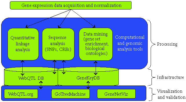
A process overview.

QTL MAPPING

Experimental design

Microarrays provide an extraordinarily efficient tool to obtain very large numbers of quantitative assays from tissue samples. For example, using the Affymetrix M430 arrays one can obtain approximately 45 000 measurements of relative mRNA abundance from a whole tissue such as the brain or from a single cell population, such as hematopoietic stem cells. In much of our recent work we have used the Affymetrix U74Av2 array to estimate the abundance of 12 422 transcripts from the mouse brain. The design of our experiments is quite simple. We extract mRNA from three litter-mate mice of the same strain and sex, pool the mRNA, and hybridize the sample to the microarray. We do this three times for each strain and sex (independent biological replicates). There is no intentional experimental manipulation of the animals or strains of mice. The essential feature to note in our experimental design is that the isogenic strains of mice that we study are all related yet genetically unique from one another.

RI strains

These related strains of mice collectively form what is called a “mapping panel.” The strain set that we use is called the BXD mapping panel because all of the 32 strains originate from the same two original progenitor strains: C57BL/6J (the B strain) and DBA/2J (the D strain). The 32 derivative BXD strains are genetic mosaics of the two parental strains. If one were to pick one of the 32 strains at random and examine a piece of one particular chromosome, there would be an approximately 0.5 probability of that piece having descended down through the generations from the B or the D parental strain. If one looked at the same part of a particular chromosome in all the 32 strains one would end up with a vector of genotypes. For example, the tip of chromosome 1 of BXD strains 11 through 16 might read BDBBDD. Thus there are 2³² or 4.29 × 10⁹ possible combinations of these vectors of genotypes. The chromosomes of individual BXD strains actually consist of very long stretches of B-type or D-type chromosomes. The average stretch is almost 50 million base pairs long. The entire set of 32 BXD strains incorporate sufficient recombinations between the parental chromosomes to encode a total of about 2¹¹ locations across the mouse genome. This means that in the best case one can only specify locations to about 1.27 × 10⁶ bp. An amount 1.27 million bp will typically contain 17 genes. (Of course, the locations of these recombinations is close to a random Poisson process.)

Unlike other recombinant cross progeny used for QTL analysis, all of the BXD strains are fully inbred. To make these RI strains, full siblings were mated successively for 20 generations to produce each of the 32 strains. This has been an expensive process that has made several strain sets available to the research community by commercial suppliers (The Jackson Laboratory, www.jax.org) or the originating laboratory. Making fully RI strains from a crossbreeding between the C57BL/6J and DBA/2J parental strains has taken about eight years. These strains have been used for over 20 years for the detection of QTLs in a wide range of phenotypes [8]. Additional 45 strains have been generated recently [9].

Finding the genetic regulatory locus

There are numerous genetic polymorphisms (allelic variants) that exist between the two parental strains. As an illustrative example, consider two alleles of a gene coding for a product that is absolutely required to deposit pigmentation in the hair and eye. Further let us assume that these two alleles act as a digital switch: the B allele inherited from C57BL/6J is the active form and the D allele inherited from DBA/2J is the inactive form.

In the D state, the mice are albinos; in the B state, they are normally pigmented. The vector of this phenotype across the strains might look PWWWWP (P, pigmented; W, white) for strains 11 through 16. A simple comparison of this vector of phenotypes to the vector of genotypes on the tip of chromosome 1 (BDBBDD) clearly rules out this location since the vectors do not match particularly well. A vector of genotypes on chromosome 7 at 77 million base pairs (Mb), however, is a perfect fit: BDDDDB. Depending on the coding convention that we use, this will give a correlation either of 1 or of −1. This is the central concept of mapping simple one-gene (monogenic) traits to discover one or more genotype vectors (markers) that have tight quantitative associations with the phenotype vectors across a large mapping panel. Recall however that our particular 32-strain genotype vector only provides enough resolution to get us down to a genetic neighborhood containing about 17 genes. We call this a genetic locus (sometimes called a gene locus), although we have to remember that we cannot yet assert which gene in this locus is actually the pigmentation switch.

Up to this point we have considered a trait that can be easily dichotomized. The vast majority of traits in which we are interested, however, are spread continuously over a broad range of values that often approximates a Gaussian distribution. These traits are frequently controled by more than a single genetic locus. Furthermore, environmental factors typically introduce a complementary nongenetic source of variance to a trait measured across a genetically diverse group of individuals. Consider, for example, body weight. This is a classic example of a complex highly variable population trait that is due to a multifactorial admixture of genetic factors, environmental factors, and interactions between genes and environment. Even a trait such as the amount of mRNA expressed in the brains of mice and measured using microarrays is a very complex trait. We refer the interested reader to our previous work [5, 7] for more information on this subject. The abundance of mRNA is influenced by rates of transcription, rates of splicing and degradation, stages of the circadian cycle, and a variety of other environmental factors. Many of these influences on transcript abundance exert their effects via the actions of other genes. QTL mapping of mRNA abundance allows one to detect these genetic sources of variation in gene expression [5, 7, 10, 11].

COMPUTATIONAL METHODS

A clique-centric approach

Current high-throughput molecular assays generate immense numbers of phenotypic values. Billions of individual hypotheses can be tested from a single BXD RI transcriptome profiling experiment. QTL mapping, however, tends to be highly focused on small sets of traits and genes. Many public users of our data resources approach the data with specific questions of particular gene-gene and/or gene-phenotype relationships [12]. These high-dimensional datasets are best understood when the correlated phenotypes are determined and analyzed simultaneously. Data reduction via automated extraction of coregulated gene sets from transcriptome QTL data is a challenge. Given the need to analyze efficiently tens of thousands of genes and traits, it is essential to develop tools to extract and characterize large aggregates of genes, QTLs, and highly variable traits.

There are advantages of placing our work in a graph-theoretic framework. This representation is known to be appropriate for probing and determining the structure of biological networks including the extraction of evolutionarily conserved modules of coexpressed genes. See, for example, [13, 14, 15]. A major computational bottleneck in our efforts to identify sets of putatively coregulated genes is the search for cliques, a classic graph-theoretic problem. Here a gene is denoted by a vertex, and a coexpression value is represented by the weight placed on an edge joining a pair of vertices. Clique is widely known for its application in a variety of combinatorial settings, a great number of which are relevant to computational molecular biology. See, for example, [16]. A considerable amount of effort has been devoted to solving clique efficiently. An excellent survey can be found in [17].

In the context of microarray analysis, our approach can be viewed as a form of clustering. A wealth of clustering approaches has been proposed. See [18, 19, 20, 21, 22] to list just a few. Here the usual goal is to partition vertices into disjoint subsets, so that the genes that correspond to the vertices within each subset display some measure of homogeneity. An advantage clique that holds over most traditional clustering methods is that cliques need not be disjoint. A vertex can reside in more than one (maximum or maximal) clique, just as a gene product can be involved in more than one regulatory network. There are recent clustering techniques, for example those employing factor analysis [23], that do not require exclusive cluster membership for single genes. Unfortunately, these tend to produce biologically uninterpretable factors without the incorporation of prior biological information [24]. Clique makes no such demand. Another advantage of clique is the purity of the categories it generates. There is considerable interest in solving the dense k-subgraph problem [25]. Here the focus is on a cluster's edge density, also referred to as clustering coefficient, curvature, and even cliquishness [26, 27]. In this respect, clique is the “gold standard.” A cluster's edge density is maximized with clique by definition.

The inputs to clique are an undirected graph G with n vertices, and a parameter k ≤ n. The question asked is whether G contains a clique of size k, that is, a subgraph isomorphic to K_k, the complete graph on K vertices. The importance of K_k lies in the fact that each and every pair of its vertices is joined by an edge. Subgraph isomorphism, clique in particular, is $𝒩𝒫$-complete. From this it follows that there is no known algorithm for deciding clique that runs in time polynomial in the size of the input. One could of course solve clique by generating and checking all $\left(\begin{array}{l}n\\ k\end{array}\right)$ candidate solutions. But this brute force approach requires O(n^k) time, and is thus prohibitively slow, even for problem instances of only modest size.

Our methods are employed as illustrated in Figure 2. We will concentrate our discussion on the classic maximum clique problem. Of course we also must handle the related problem of generating all maximal cliques once a suitable threshold has been chosen, which is itself often a function of maximum clique size. There are a variety of other issues dealing with preprocessing and postprocessing. Although we do not explicitly deal with them in the present paper, they are for the most part quite easily handled and are dwarfed by the computational complexity of the fundamental clique problem at the heart of our method.

Figure 2.

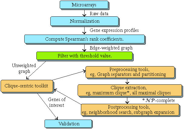
The clique-centric toolkit and its use in microarray analysis.

Fixed-parameter tractability

The origins of fixed-parameter tractability (FPT) can be traced at least as far back as the work done to show, via the graph minor Theorem, that a variety of parameterized problems are tractable when the relevant input parameter is fixed. See, for example, [28, 29]. Formally, a problem is FPT if it has an algorithm that runs in O(f(k)n^c), where n is the problem size, k is the input parameter, and c is a constant independent of both n and k [30]. Unfortunately, clique is not FPT unless the $𝒲$ hierarchy collapses. (The $𝒲$ hierarchy, whose lowest level is FPT, can be viewed as a fixed-parameter analog of the polynomial hierarchy, whose lowest level is $𝒫$.) Thus we focus instead on clique's complementary dual, the vertex cover problem. Consider $\overline{G}$, the complement of G. ($\overline{G}$ has the same vertex set as G, but edges present in G are absent in $\overline{G}$ and vice versa.) As with clique, the inputs to vertex cover are an undirected graph G with n vertices, and a parameter k ≤ n. The question now asked is whether G contains a set C of k vertices that covers every edge in G, where an edge is said to be covered if either or both of its endpoints are in C. Like clique, vertex cover is $𝒩𝒫$-complete. Unlike clique, however, vertex cover is also FPT. The crucial observation here is this: a vertex cover of size k in $\overline{G}$ turns out to be exactly the complement of a clique of size n − k in G. Thus, we search for a minimum vertex cover in $\overline{G}$, thereby finding the desired maximum clique in G. Currently, the fastest known vertex cover algorithm runs in O(1.2852^k + kn) time [31]. Contrast this with O(n^k). The requisite exponential growth (assuming $𝒫$≠$𝒩𝒫$) is therefore reduced to a mere additive term.

Kernelization, branching, parallelization, and load balancing

The initial goal is to reduce an arbitrary input instance down to a relatively small computational kernel, then decomposing it so that an efficient, systematic search can be conducted. Attaining a kernel whose size is quadratic in k is relatively straightforward [32]. Ensuring a kernel whose size is linear in k has until recently required much more powerful and considerably slower methods that rely on linear programming relaxation [33, 34].

In [35], we introduced and analyzed a new technique, termed crown reduction. A crown is an ordered pair (I, H) of subsets of vertices from G that satisfies the following criteria: (1) $I\ne \varnothing$ is an independent set of G, (2) H = N(I), and (3) there exists a matching M on the edges connecting I and H such that all elements of H are matched. H is called the head of the crown. The width of the crown is |H|. This notion is depicted in Figure 3.

Figure 3.

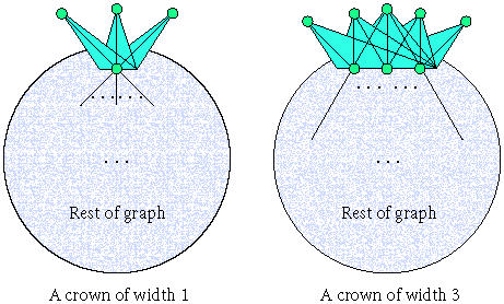
Sample crown decompositions.

Theorem (see[35]). Any graph G can be decomposed into a crown (I, H) for which H contains a minimum-size vertex cover of G and so that |H| ≤ 3k. Moreover, the decomposition can be accomplished in O(n^5/2) time.

The problem now becomes one of exploring the kernel efficiently. A branching process is carried out using a binary search tree. Internal nodes represent choices; leaves denote candidate solutions. Subtrees spawned off at each level can be explored in parallel. The best results have generally been obtained with minimal intervention, in the extreme case launching secure shells (SSHs) [36]. To maintain scalability as datasets grow in size and as more machines are brought on line, some form of dynamic load balancing is generally required. We have implemented such a scheme using sockets and process-independent forking. Results on 32–64 processors in the context of motif discovery are reported in [37]. Large-scale testing using immense genomic and proteomic datasets are reported in [38].

SAMPLE COMPUTATIONAL RESULTS

We are now able to solve real, nonsynthetic instances of clique on graphs whose vertices number in the thousands. (Just imagine a straightforward O(n^k) algorithm on problems of that size!)

To illustrate, we recently solved a problem on Mus musculus neurogenetic microarray data with 12 422 vertices (probe sets). With expression values normalized to [0, 1] and the threshold set at 0.5, the clique we returned (via vertex cover) denoted a set of 369 genes that appear experimentally to be coregulated. This took a few days to solve even with our best current methods. Yet solving it at all was probably unthinkable just a short time ago. After iterating across several threshold choices, a value of 0.85 was selected for detailed study. For this graph, G, the maximum clique size is 17. Because it is difficult to visualize G, we employ a clique intersection graph, C_G, as follows. Each maximal clique of size 15 or more in G is represented by a vertex in C_G. An edge connects a pair of vertices in C_G if and only if the intersection of the corresponding cliques in G contains at least 13 members. C_G is depicted in Figure 4, with vertices representing cliques of size 15 (in green), cliques of size 16 (in black), and cliques of size 17 (in red). One rather surprising result is that the gene found most often across large maximal cliques is Veli3 (aka Lin7c). This appears not to be due to some so-called “housekeeping” function, but instead because the relatively unstudied Veli3 is in fact central to neurological function [39, 40].

Figure 4.

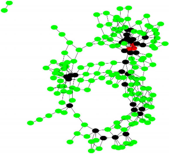
A clique intersection graph for a large microarray dataset.

CLIQUES OF HIGHLY CORRELATED TRANSCRIPTS AND BEHAVIORAL PHENOTYPES

We can infer that coexpression of genes in mice of common genetic background is due to a shared regulatory mechanism, because the correlation is between trait means from different lines of mice, rather than from within an experimental group. Clique membership alone does not tell us anything about the basis of common genetic regulation. By combining clique data with QTL analysis, the regulatory loci underlying the shared genetic mediation of gene expression can be identified. This allows us to determine the impact of genetic variability in gene expression on other biological processes. Using the aforementioned stringent correlation threshold of 0.85, the most highly connected transcript identified was that of Veli3. One maximal clique of seventeen highly associated transcript abundances includes several nuclear proteins. A single principal component of these transcripts accounts for 95% of the total genetic sample variance.

No single QTL can be found for the members of this clique, but a multiple QTL mapping analysis reveals an interacting pair of loci on chromosomes 12 and X, at markers D12Mit46 (29.163 Mb) and DXMit117 (110.670 Mb). See Figure 5, which shows the results from a search for pairs of genetic loci that modulate expression of a clique. Chromosomes 12, 19, and X are shown. Likelihood ratio statistics for multiple QTL models are plotted on the pseudocolor scale. The upper left triangle shows fit results for an interaction model, and the lower right triangle shows fit results for a model containing both additive and interaction effects of the two loci. The joint model including markers on 12 and X is significant (P < .05) by permutation analysis. A D allele at both loci results in low levels of the phenotype and a B allele at both loci results in a high level of the phenotype. The chromosome 12 locus is the physical location of two clique members: B cell receptor associated protein Bcap29, and myelin transcription factor 1-like protein, Myt1l. An interesting functional and positional candidate at the Chromosome X locus is integral membrane protein 1, Itm1. While this is not a member of the clique we are analyzing here, it does frequently cooccur along with Veli3 in many maximal cliques.

Figure 5.

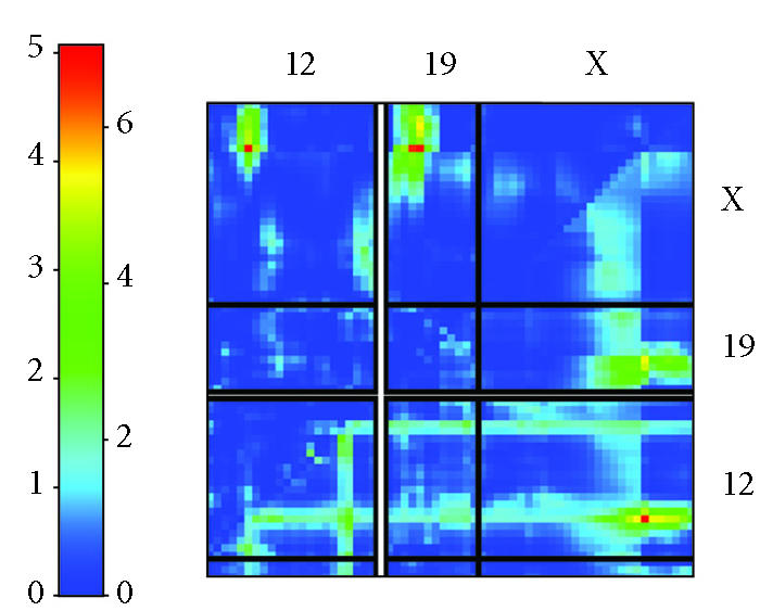
Multiple QTL mapping analysis. In the upper left triangle, a pseudo-color plot shows the likelihood ratio statistic for each two-locus interaction. In the lower right triangle, a likelihood ratio statistic is depicted for the full two-locus model, which fits additive effects for each pair of loci and their interaction. Significance was assessed by genome-wide permutation analysis.

In addition to tens of thousands of transcript traits, we have assembled a database of over 600 organismic phenotypes, including many morphometric traits. An understanding of the genetic control of these phenotypes can help explain their evolution. In the present example, we have found the previously mentioned clique to associate with behavioral and metabolic phenotypes. This clique correlates with both midbrain iron levels, and locomotor behavior. Interestingly, one of the clique members, Gs2na (GS2 nuclear autoantigen), that, at 46.048 Mb on chromosome 12, is a little too far afield to be a positional QTL candidate gene, is a striatin family member and the negative correlation we observe between clique expression and locomotor behavior is consistent with literature reports of locomotor impairment associated with decreased levels of striatin [41]. At this point research becomes hypothesis driven; indeed, the result of this collaborative analysis is a simple testable hypothesis, extracted from many billions of data relations. We are now in the process of evaluating the hypothesis that genetic variation in iron metabolism influences expression of the Veli3 clique members in the brain and consequently affects locomotor activity.

INTEGRATIVE GENOMIC DATA MINING

GeneKeyDB

High-throughput, high volume data like these gene expression data from genetically variant mice should be examined in a biological context. The subsets of interesting genes must be analyzed, in part, by using existing information that describe the role these genes play in biological processes. When computing and navigating these data in terms of graphs and networks, we need to have a way to manipulate various kinds of metadata about sets of genes and gene products.

We have developed several such tools for genes and gene products that are discovered from the clique and QTL data analysis. Most gene-centered data resources that are generally available for retrieving metadata about genes are displayed and manipulated in a one-gene-at-a-time format (eg, Entrez Gene). We have developed a lightweight data mining environment that allows the automated integration of various types of data about sets of genes. This environment is called GeneKeyDB. This system includes metadata from GenBank, Entrez Gene, Ensembl, and several other well-established biological databases. GeneKeyDB uses a relational database backend to facilitate interactions between tools and data. Among other functions, GeneKeyDB automatically converts the different database identifiers from these different databases. It can, for example, start with GenBank cDNA identifiers, locate the “sequence feature” information from genome sequence data entries, and assist in retrieving sequences for detailed analyses. GeneKeyDB can also obtain various kinds of homologs, functional annotation, or other attributes of genes and gene products. Furthermore, it serves as a repository for results that are created by our computational tools.

We have devised two types of computational analyses that are supported by the underlying GeneKeyDB system.

GoTreeMachine

Gene ontology (GO) produces structured, precisely defined, common, controled vocabulary for describing the roles of genes and gene products [42]. GO has been used frequently in the functional profiling of high-throughput data. We have developed a web-based tool, GOTM, for the analysis and visualization of sets of genes using GO hierarchies [7]. Besides being a stand-alone functional profiling tool, GOTM can work with other computational tools for gene set centered integrated analysis. GOTM has been employed in various ways in this respect. This includes WebQTL's use of GOTM to narrow down candidate gene lists and generate functional profiles for genes in a relevance network or genes correlated to complex phenotypes.

We use ontology analysis to evaluate the functional significance of the cliques found by our graph algorithms, and prioritize the cliques for further study. Figure 6 depicts a clique of size eight that was detected within the gene coexpression network constructed using the microarray data from the RI mouse lines. The five green vertices denote genes that belong to the GO functional category of “DNA binding.” The red vertices denote genes that either have no annotation or are annotated as function “unknown.” If we randomly pick five genes from all annotated genes on the microarray, the expected frequency of genes in the category DNA binding is only 0.9. The chance of finding all five genes in the category DNA binding is P = .00051 as calculated by the hypergeometric test implemented in GOTM. Out of the 5227 maximal cliques we generated, ontology analysis has detected a total of 342 of them that are significantly enriched in one or more GO categories (P < .01). The clique shown in Figure 6 has a P value less than .001, and is one of several cliques we are studying. Note the presence of the gene Veli3.

Figure 6.

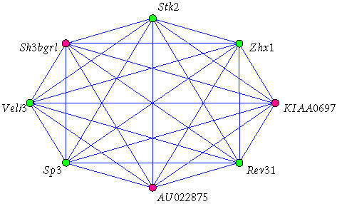
A relevant clique containing Veli3

Batch sequence analysis

We are also deploying integrative methods that attempt to predict cis-regulatory elements (CREs) in the upstream regions from sets of genes that are putatively coregulated. These CREs are thought to be the DNA sites to which protein regulatory transcription factors preferentially bind in promoters or enhancers and exert regulatory control of gene expression. We are combining a number of analyses to look at sets of CREs that are found in a subset of genes that seems to show strong coregulation and are consistent with the clique and QTL data.

We have assembled a pipeline, batch sequence analysis (BSA), that can retrieve the sequence data for the target genes and their orthologous counterparts in other chordate organisms. This pipeline carries out a number of processes that enable us to use both coregulated gene sets and phylogenetic footprinting in an integrated pipeline to identify putative CREs. An important advantage of the pipeline is its ability to define the evolutionarily conserved non-coding sequences, which are thought to contain most of the CREs [43]. This should substantially reduce the noise levels. BSA can be carried out in a high throughput, automated process because of the underlying GeneKeyDB infrastructure. BSA is routinely using both multiple Em for motif elicitation (MEME) and motif alignment and search tool (MAST) as part of the sequence analysis, but other motif finding and searching methods are under development. A set of CRE motifs can be found in cliques or other interesting subsets of genes with motif searches (like MEME). We can then use MAST or similar searching tools to take those sets of putative CREs to do a global search for all possible targets in a database that contains promoter sequences from all human, mouse, and rat genes. The latter step could help define new genes that are targets of a gene regulatory network that were not initially identified. The BSA pipeline stores its results in the GeneKeyDB relational database.

SUMMARY AND DIRECTIONS FOR FUTURE RESEARCH

Our current work demonstrates the use of clique to extract signal from large genetic correlation matrices. We also employ genome-scale tools to interpret the shared molecular function, biological process, cellular localization, and sequence motifs of clique members. Despite what has been accomplished in the BXD lines, the size of existing RI strain sets limits the power and resolution of this technique. The Complex Trait Consortium plans to expand this set with the development of a 1024 RI strain panel [44]. The creation of this resource will greatly increase the depth of our analysis. The breadth of the analysis can be expanded almost indefinitely. Although the work we have described here has been restricted to the analysis of gene expression microarray phenotypes, any attribute of these strains that can be measured can in principle be incorporated into the genetic correlation matrix. We already have a wealth of data on microscale and macroscale biological phenotypes ranging from cellular responses to behavior. Novel high-throughput molecular phenotypes will greatly expand this collection. To accomodate such vast increases in data dimensionality, we are currently in the process of porting our codes to supercomputers at Oak Ridge National Laboratory (ORNL) (Tennessee, USA). These are difficult tasks indeed, given the many novel features of our algorithms. Great care is required to manage processor and memory resources. Load balancing can be especially problematic [37]. Initial targets include a 256-node SGI Altix and a 256-node Cray X1. In the longer term, we aim to employ the tremendously more powerful machines now under construction and awarded to ORNL in the recent competition to build the nation's next leadership-class computing facility for science. We believe that with our algorithms and these platforms we can solve the problem instances previously considered hopelessly out of reach.

References

- 1.Williams R.W, Gu J, Qi S, Lu L. The genetic structure of recombinant inbred mice: High-resolution consensus maps for complex trait analysis. Genome Biol. 2001;2(11):Research0046. doi: 10.1186/gb-2001-2-11-research0046. [DOI] [PMC free article] [PubMed] [Google Scholar]
- 2.Airey D.C, Shou S, Lu L, Williams R.W. Genetic sources of individual differences in the cerebellum. Cerebellum. 2002;1(4):233–240. doi: 10.1080/147342202320883542. [DOI] [PubMed] [Google Scholar]
- 3.Peirce J.L, Chesler E.J, Williams R.W, Lu L. Genetic architecture of the mouse hippocampus: Identification of gene loci with selective regional effects. Genes Brain Behav. 2003;2(4):238–252. doi: 10.1034/j.1601-183x.2003.00030.x. [DOI] [PubMed] [Google Scholar]
- 4.Flint J. Analysis of quantitative trait loci that influence animal behavior. J Neurobiol. 2003;54(1):46–77. doi: 10.1002/neu.10161. [DOI] [PubMed] [Google Scholar]
- 5.Chesler E.J, Wang J, Lu L, Qu Y, Manly K.F, Williams R.W. Genetic correlates of gene expression in recombinant inbred strains: A relational model system to explore neurobehavioral phenotypes. Neuroinformatics. 2003;1(4):343–357. doi: 10.1385/NI:1:4:343. [DOI] [PubMed] [Google Scholar]
- 6.Wang J, Williams R.W, Manly K.F. WebQTL: web-based complex trait analysis. Neuroinformatics. 2003;1(4):299–308. doi: 10.1385/NI:1:4:299. [DOI] [PubMed] [Google Scholar]
- 7.Zhang B, Schmoyer D, Kirov S, Snoddy J. GOTree Machine (GOTM): a web-based platform for interpreting sets of interesting genes using gene ontology hierarchies. BMC Bioinformatics. 2004;5(1):16. doi: 10.1186/1471-2105-5-16. [DOI] [PMC free article] [PubMed] [Google Scholar]
- 8.Taylor B.A, Wnek C, Kotlus B.S, Roemer N, MacTaggart T, Phillips S.J. Genotyping new BXD recombinant inbred mouse strains and comparison of BXD and consensus maps. Mamm Genome. 1999;10(4):335–348. doi: 10.1007/s003359900998. [DOI] [PubMed] [Google Scholar]
- 9.Peirce J.L, Lu L, Gu J, Silver L.M, Williams R.W. A new set of BXD recombinant inbred lines from advanced intercross populations in mice. BMC Genet. 2004;5(1):7. doi: 10.1186/1471-2156-5-7. [DOI] [PMC free article] [PubMed] [Google Scholar]
- 10.Brem R.B, Yvert G, Clinton R, Kruglyak L. Genetic dissection of transcriptional regulation in budding yeast. Science. 2002;296(5568):752–755. doi: 10.1126/science.1069516. [DOI] [PubMed] [Google Scholar]
- 11.Schadt E.E, Monks S.A, Drake T.A, et al. Genetics of gene expression surveyed in maize, mouse and man. Nature. 2003;422(6929):297–302. doi: 10.1038/nature01434. [DOI] [PubMed] [Google Scholar]
- 12.Chesler E.J, Lu L, Wang J, Williams R.W, Manly K.F. WebQTL: rapid exploratory analysis of gene expression and genetic networks for brain and behavior. Nat Neurosci. 2004;7(5):485–486. doi: 10.1038/nn0504-485. [DOI] [PubMed] [Google Scholar]
- 13.Alon U. Biological networks: the tinkerer as an engineer. Science. 2003;301(5641):1866–1867. doi: 10.1126/science.1089072. [DOI] [PubMed] [Google Scholar]
- 14.Barabasi A.L, Oltvai Z.N. Network biology: understanding the cell's functional organization. Nat Rev Genet. 2004;5(2):101–113. doi: 10.1038/nrg1272. [DOI] [PubMed] [Google Scholar]
- 15.Oltvai Z.N, Barabasi A.L. Systems biology. Life's complexity pyramid. Science. 2002;298(5594):763–764. doi: 10.1126/science.1078563. [DOI] [PubMed] [Google Scholar]
- 16.Setubal J.C, Meidanis J. Introduction to Computational Molecular Biology. Boston, Mass: PWS Publishing Company; 1997. [Google Scholar]
- 17.Bomze I.M, Budinich M, Pardalos P.M, Pelillo M. The maximum clique problem. In: Du D-Z, Pardalos P.M, editors; Handbook of Combinatorial Optimization (Supplement Volume A) vol. 4. Boston, Mass: Kluwer Academic Publishers; 1999. pp. 1–74. [Google Scholar]
- 18.Bellaachia A, Portnoy D, Chen Y, Elkahloun A.G, editors. ECAST: a data mining algorithm for gene expression data. In: 2nd Workshop on Data Mining in Bioinformatics (BIOKDD 2002); Alberta, Canada. 2002. pp. 49–54. [Google Scholar]
- 19.Ben-Dor A, Bruhn L, Friedman N, Nachman I, Schummer M, Yakhini Z. Tissue classification with gene expression profiles. J Comput Biol. 2000;7(3-4):559–583. doi: 10.1089/106652700750050943. [DOI] [PubMed] [Google Scholar]
- 20.Ben-Dor A, Shamir R, Yakhini Z. Clustering gene expression patterns. J Comput Biol. 1999;6(3-4):281–297. doi: 10.1089/106652799318274. [DOI] [PubMed] [Google Scholar]
- 21.Hansen P, Jaumard B. Cluster analysis and mathematical programming. Math Program. 1997;79(1-3):191–215. [Google Scholar]
- 22.Hartuv E, Schmitt A, Lange J, Meier-Ewert S, Lehrachs H, Shamir R, editors. An algorithm for clustering cDNAs for gene expression analysis. In: Proceedings of the 3rd Annual International Conference on Computational Molecular Biology (RECOMB '99); Lyon, France. 1999. pp. 188–197. [Google Scholar]
- 23.Alter O, Brown P.O, Botstein D. Singular value decomposition for genome-wide expression data processing and modeling. Proc Natl Acad Sci USA. 2000;97(18):10101–10106. doi: 10.1073/pnas.97.18.10101. [DOI] [PMC free article] [PubMed] [Google Scholar]
- 24.Girolami M, Breitling R. Biologically valid linear factor models of gene expression. Bioinformatics. 2004;20(17):3021–3033. doi: 10.1093/bioinformatics/bth354. [DOI] [PubMed] [Google Scholar]
- 25.Feige U, Peleg D, Kortsarz G. The dense k-subgraph problem. Algorithmica. 2001;29:410–421. [Google Scholar]
- 26.Rougemont J, Hingamp P. DNA microarray data and contextual analysis of correlation graphs. BMC Bioinformatics. 2003;4(1):15. doi: 10.1186/1471-2105-4-15. [DOI] [PMC free article] [PubMed] [Google Scholar]
- 27.Watts D.J, Strogatz S.H. Collective dynamics of “small-world” networks. Nature. 1998;393(6684):440–442. doi: 10.1038/30918. [DOI] [PubMed] [Google Scholar]
- 28.Fellows M.R, Langston M.A. Nonconstructive tools for proving polynomial-time decidability. J ACM. 1988;35(3):727–739. [Google Scholar]
- 29.Fellows M.R, Langston M.A. On search, decision and the efficiency of polynomial-time algorithms. Journal of Computer and Systems Science. 1994;49:769–779. [Google Scholar]
- 30.Downey R.G, Fellows M.R. Parameterized Complexity. Berlin: Springer; 1999. [Google Scholar]
- 31.Chen J, Kanj I.A, Jia W. Vertex cover: further observations and further improvements. J Algorithms. 2001;41:280–301. [Google Scholar]
- 32.Buss J.F, Goldsmith J. Nondeterminism within 𝒫. SIAM J Comput. 1993;22(3):560–572. [Google Scholar]
- 33.Khuller S. The vertex cover problem. SIGACT News. 2002;33:31–33. [Google Scholar]
- 34.Nemhauser G.L, Trotter L.E. Vertex packing: Structural properties and algorithms. Math Program. 1975;8:232–248. [Google Scholar]
- 35.Abu-Khzam F.N, Collins R.L, Fellows M.R, Langston M.A, Suters W.H, Symons C.T, editors. Kernelization algorithms for the vertex cover problem: Theory and experiments. In: Proceedings ACM-SIAM Workshop on Algorithm Engineering and Experiments (ALENEX '04); New Orleans, La. 2004. [Google Scholar]
- 36.Abu-Khzam F.N, Langston M.A, Shanbhag P, editors. Scalable parallel algorithms for difficult combinatorial problems: A case study in optimization. In: Proceedings, International Conference on Parallel and Distributed Computing and Systems (PDCS '03); California. 2003. pp. 563–568. [Google Scholar]
- 37.Baldwin N.E, Collins R.L, Langston M.A, Leuze M.R, Symons C.T, Voy B.H, editors. High performance computational tools for motif discovery. In: Proceedings IEEE International Workshop on High Performance Computational Biology (HiCOMB '04); Santa Fe, New Mexico. 2004. [Google Scholar]
- 38.Abu-Khzam F.N, Langston M.A, Shanbhag P, Symons C.T. Technical Report UT-CS-04-524. Knoxville, Tenn: The University of Tennessee; 2004. Scalable Parallel Algorithms for FPT Problems. [Google Scholar]
- 39.Becamel C, Alonso G, Galeotti N, et al. Synaptic multiprotein complexes associated with 5-HT(2C) receptors: a proteomic approach. EMBO J. 2002;21(10):2332–2342. doi: 10.1093/emboj/21.10.2332. [DOI] [PMC free article] [PubMed] [Google Scholar]
- 40.Butz S, Okamoto M, Sudhof T.C. A tripartite protein complex with the potential to couple synaptic vesicle exocytosis to cell adhesion in brain. Cell. 1998;94(6):773–782. doi: 10.1016/s0092-8674(00)81736-5. [DOI] [PubMed] [Google Scholar]
- 41.Bartoli M, Ternaux J.P, Forni C, et al. Down-regulation of striatin, a neuronal calmodulin-binding protein, impairs rat locomotor activity. J Neurobiol. 1999;40(2):234–243. [PubMed] [Google Scholar]
- 42.Ashburner M, Ball C.A, Blake J.A. In vitro production of secondary metabolites by cultivated plant cells: the crucial role of the cell nutritional status. Nat Genet. 2000;25(1):25–29. [Google Scholar]
- 43.Wasserman W.W, Palumbo M, Thompson W, Fickett J.W, Lawrence C.E. Human-mouse genome comparisons to locate regulatory sites. Nat Genet. 2000;26(2):225–228. doi: 10.1038/79965. [DOI] [PubMed] [Google Scholar]
- 44.Vogel G. Genetics. Scientists dream of 1001 complex mice. Science. 2003;301(5632):456–457. doi: 10.1126/science.301.5632.456. [DOI] [PubMed] [Google Scholar]