Functional Clustering Algorithm for High-Dimensional Proteomics Data

Abstract

Clustering proteomics data is a challenging problem for any traditional clustering algorithm. Usually, the number of samples is largely smaller than the number of protein peaks. The use of a clustering algorithm which does not take into consideration the number of features of variables (here the number of peaks) is needed. An innovative hierarchical clustering algorithm may be a good approach. We propose here a new dissimilarity measure for the hierarchical clustering combined with a functional data analysis. We present a specific application of functional data analysis (FDA) to a high-throughput proteomics study. The high performance of the proposed algorithm is compared to two popular dissimilarity measures in the clustering of normal and human T-cell leukemia virus type 1 (HTLV-1)-infected patients samples.

INTRODUCTION

A variety of mass spectrometry-based platforms are currently available for providing information on both protein patterns and protein identity [1, 2]. Specifically, the first widely used such mass spectrometric technique is known as surface-enhanced laser desorption ionization (SELDI) coupled with time-of-flight (TOF) mass spectrometric detection [3, 4, 5]. The SELDI approach is based on the use of an energy-absorbing matrix such as sinapinic acid (SPH), large molecules such as peptides ionize instead of decomposing when subjected to a nitrogen UV laser. Thus, partially purified serum is crystallized with an SPH matrix and placed on a metal slide. Depending upon the range of masses the investigator wishes to study, there are a variety of possible slide surfaces; for example, the strong anion exchange (SAX) or the weak cation exchange (WCX) surface. The peptides are ionized by the pulsed laser beam and then traverse a magnetic-field-containing column. Masses are separated according to their TOFs as the latter are proportional to the square of the mass-to-charge (m/z) ratio. Since nearly all of the resulting ions have unit charge, the mass-to-charge ratio is in most cases a mass. The spectrum (intensity level as a function of mass) is recorded, so the resulting data obtained on each serum sample are a series of intensity levels at each mass value on a common grid of masses (peaks).

Proteomic profiling is a new approach to clinical diagnosis, and many computational challenges still exist. Not only are the platforms themselves still improving, but the methods used to interpret the high-dimensional data are developing as well [6, 7].

A variety of clustering approaches has been applied to high-dimensional genomics and proteomics data [8, 9, 10, 11]. Hierarchical clustering methods give rise to nested partitions, meaning the intersection of a set in the partition at one level of the hierarchy with a set of the partition at a higher level of the hierarchy will always be equal to the set from the lower level or the empty set. The hierarchy can thus be graphically represented by a tree.

Functional data analysis (FDA) is a statistical data analysis represented by smooth curves or continuous functions μ_i(t), i = 1, . . ., n, where n is the number of observations and t might or might not necessarily denote time but might have a general meaning. Here t denotes the mass (m/z). In practice, the information over μ_i(t) is collected at a finite number of points, T_i, thus observing the data vector y_i = (y_i1, . . ., y_iTi)^t. The basic statistical model of FDA is given by

$$\begin{array}{c}{y}_{ij}={\widehat{\mu }}_i\left(t_{ij}\right)={\mu }_i\left(t_{ij}\right)+{ϵ}_i\left(t_{ij}\right),\\ i=1,\dots ,n,j=1,\dots ,T_i,\end{array}\left(1\right)$$

where t_ij is the mass value at which the jth measurement is taken for the ith function μ_i. The independent disturbance terms ϵ_i(t_ij) are responsible for roughness in y_i. FDA has been developed for analyzing functional (or curve) data. In FDA, data consists of functions not of vectors. Samples are taken at time points t₁, t₂, . . ., and regard μ_i(t_ij) as multivariate observations. In this sense the original functional y_ij can be regarded as the limit of μ_i(t_ij) as the sampling interval tends to zero and the dimension of multivariate observations tends to infinity. Ramsay and Silverman [12, 13] have discussed several methods for analyzing functional data, including functional regression analysis, functional principal component analysis (PCA), and functional canonical correlation analysis (CCA). These methodologies look attractive, because one often meets the cases where one wishes to apply regression analysis and PCA to such data. In the following we describe how to use the FDA tools for applying FDA and a new dissimilarity measure to classify the spectra data.

We propose to implement a hierarchical clustering algorithm for proteomics data using FDA. We use functional transformation to smooth and reduce the dimensionality of the spectra and develop a new algorithm for clustering high-dimensional proteomics data.

MATERIAL AND METHODS

Serum samples from HTLV-1-infected patients

Protein expression profiles generated through SELDI analysis of sera from human t-cell leukemia virus type 1- (HTLV-1)-infected individuals were used to determine the changes in the cell proteome that characterize adult T-cell leukemia (ATL), an aggressive lymphoproliferative disease from HTLV-1-associated myelopathy/tropical spastic paraparesis (HAM/TSP), a chronic progressive neurodegenerative disease. Both diseases are associated with the infection of T cells by HTLV-1. The HTLV-1 virally encoded oncoprotein Tax has been implicated in the retrovirus-mediated cellular transformation and is believed to contribute to the oncogenic process through induction of genomic instability affecting both DNA repair integrity and cell cycle progression [14, 15]. Serum samples were obtained from the Virginia Prostate Center Tissue and body fluid bank. All samples had been procured from consenting patients according to protocols approved by the Institutional Review Board and stored frozen. None of the samples had been thawed more than twice.

Triplicate serum samples (n = 68) from healthy or normal (n₁ = 37), ATL (n₂ = 20), and HAM (n₃ = 11) patients were processed. A bioprocessor, which holds 12 chips in place, was used to process 96 samples at one time. Each chip contained one “QC spot” from normal pooled serum, which was applied to each chip along with the test samples in a random fashion. The QC spots served as quality control for assay and chip variability. The samples were blinded for the technicians who processed the samples. The reproducibility of the SELDI spectra, that is, mass and intensity from array to array on a single chip (intra-assay) and between chips (interassay), was determined with the pooled normal serum QC sample (Figure 1).

Figure 1.

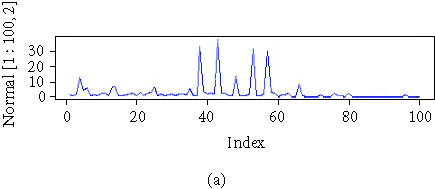
Three cut expressions from a normal, an HAM, and an ATL patient.

SELDI mass spectrometry

Serum samples were analyzed by SELDI mass spectrometry as described earlier [16]. The spectral data generated was used in this study for the development of the novel FDA.

Hierarchical clustering using functional data analysis

We propose to implement a hierarchical clustering algorithm for proteomics data using FDA, which consists of detecting hidden group structures within a functional dataset. We apply a new dissimilarity measure to the smoothed (transformed) proteomics functions ${\widehat{\mu }}_i$. Then we develop a new metric that calculates the dissimilarity between different curves produced by protein expression. The development of metrics for curve and time-series models was first addressed by Piccolo [17] and Corduas [18]. Heckman and Zamar proposed a dissimilarity measure δ_HZ for clustering curves [19]. Their dissimilarity measure considers curve invariance under monotone transformations. Let ${\Lambda }_i=\left\{{\lambda }_1^{\left(i\right)},{\lambda }_2^{\left(i\right)},\dots ,{\lambda }_{m_i}^{\left(i\right)}\right\}$ be the collection of the estimated points where the curve μ_i(t) has a local maximum and let m_i be the number of maximals per observation or per sample (i) . δ_HZ is defined as

$${\delta }_{HZ}\left(i,l\right)=\frac{{\sum }_{j=1}^{m_i}\left(r\left({\lambda }_j^{\left(i\right)}\right)-r\overline{\left({\lambda }^{\left(i\right)}\right)}\right)\left(r\left({\lambda }_j^{\left(l\right)}\right)-r\overline{\left({\lambda }^{\left(l\right)}\right)}\right)}{{{\sum }_{j=1}^{m_i}{\left(r\left({\lambda }_j^{\left(i\right)}\right)-r\overline{\left({\lambda }^{\left(i\right)}\right)}\right)}^2{\sum }_{j=1}^{m_l}\left(r\left({\lambda }^{\left(l\right)}\right)-r\overline{\left({\lambda }^{\left(l\right)}\right)}\right)}^2},\left(2\right)$$

where

$$\begin{array}{c}r\left({\lambda }_j^{\left(i\right)}\right)=k_j^{\left(i\right)}+\frac{u_j^{\left(i\right)}}{2},k_j^{\left(i\right)}=\left\{\#i,{\lambda }_i^{\left(i\right)}<{\lambda }_j^{\left(i\right)}\right\},\\ u_j^{\left(i\right)}=\left\{\#i,{\lambda }_i^{\left(i\right)}={\lambda }_j^{\left(i\right)}\right\},\overline{r\left({\lambda }^{\left(i\right)}\right)}=\frac{1}{m_i}\sum _{j=1}^{m_i}r\left({\lambda }_j^{\left(i\right)}\right).\end{array}\left(3\right)$$

This measure is powerful for regression curves which are mainly monotone. On the other hand, Cerioli et al [20] propose a dissimilarity measure δ_C extending the one proposed by Ingrassia et al [21]. Cerioli's dissimilarity δ_C is defined by

$$\begin{array}{c}d\left(i,l\right)=\sum _{j=1}^{m_i}\frac{\left|{\lambda }_j^{\left(i\right)}-{\lambda }_{\ast j}^{\left(l\right)}\right|}{m_i},\\ {\lambda }_{\ast j}^{\left(l\right)}=\left\{{\lambda }_{j^{\prime }}^{\left(l\right)}:\left|{\lambda }_j^{\left(i\right)}-{\lambda }_{j^{\prime }}^{\left(l\right)}\right|=min,i=1,\dots ,n\right\},\\ {\delta }_C\left(i,l\right)=\left(\frac{d_{il}+d_{li}}{2}\right).\end{array}\left(4\right)$$

Both dissimilarity measures show good performance for time-series data. Dissimilarity δ_C does not involve all the indices m_i of the smoothed curve. It also uses the shortest distance between curves by involving few data points obtained by FDA smoothing.

A flexible dissimilarity measure is the one that may combine the characteristic of both measures δ_HZ and δ_C. This means that a potential dissimilarity measure should use the collected estimated points of the original curve obtained from FDA so that no information is lost and should work on different type of smoothed curves without using the monotonicity restriction.

In this sense, we propose a functional-based dissimilarity δ_B measure which uses the rank of the curve proposed by Heckman and Zamar and generalizes Cerioli et al dissimilarity measure as follows:

$$\begin{array}{c}{d}_{il}=\sum _{j=1}^{m_i}\frac{\left|r\left({\lambda }_j^{\left(i\right)}\right)-r\left({\lambda }_{\ast j}^{\left(l\right)}\right)\right|}{m_i},\\ r\left({\lambda }_{\ast j}^{\left(l\right)}\right)=\frac{{\sum }_{h=1}^{m_l}\left|r\left({\lambda }_j^{\left(i\right)}\right)-r\left({\lambda }_{h^{\prime }}^{\left(l\right)}\right)\right|}{m_l},\\ r\left({\lambda }_j^{\left(i\right)}\right)=k_j^{\left(i\right)}+\frac{u_j^{\left(i\right)}}{2},k_j^{\left(i\right)}=\left\{\#i,{\lambda }_i^{\left(i\right)}<{\lambda }_j^{\left(i\right)}\right\},\\ u_j^{\left(i\right)}=\left\{\#i,{\lambda }_i^{\left(i\right)}={\lambda }_j^{\left(i\right)}\right\},\overline{r\left({\lambda }^{\left(i\right)}\right)}=\frac{1}{m_i}\sum _{j=1}^{m_i}r\left({\lambda }_j^{\left(i\right)}\right).\end{array}\left(5\right)$$

Obviously, d_ii = 0 and d_il = 0, if μ_i and μ_l have the same shape (T_i = T_l). We can adjust the formula above to obtain a dissimilarity measure that satisfies symmetry, by taking δ_B as our proposed dissimilarity measure:

$${\delta }_B\left(i,l\right)=\left(\frac{d_{il}+d_{li}}{2}\right).\left(6\right)$$

We used three powerful hierarchical methods to derive clusters or patterns using δ_B and we compare the performance of δ_B to δ_C and δ_HZ. The hierarchical algorithms we used are (1) Pam which partitions the data into different clusters “around their medoids,” (2) Clara which works as in “Pam.” Once the number of clusters is specified and representative objects have been selected from the sub-dataset, each observation of the entire dataset is assigned to the nearest medoid [22]. The sum of the dissimilarities of the observations to their closest medoid is used as a measure of the quality of the clustering. The sub-dataset for which the sum is minimal, is retained. Each sub-dataset is forced to contain the medoids obtained from the best sub-dataset until then. (3) Diana is probably unique in computing a divisive hierarchy, whereas most other software for hierarchical clustering is agglomerative. Moreover, Diana provides the divisive coefficient which measures the amount of clustering structure found. The Diana-algorithm constructs a hierarchy of clustering starting with one large cluster containing all n observations. Clusters are divided until each cluster contains only a single observation. At each stage, the cluster with the largest diameter is selected [22].

RESULTS

Functional data transformation reduces the dimensionality of the spectra

The spectral data were collected from proteomics analysis of a total number of serum samples (n = 68) including healthy or normal (n₁ = 37), ATL (n₂ = 20), and HAM (n₃ = 11) patients. The dataset is represented by an n × p matrix X, where p = 25, 196 is the number of variables (peaks) measured on each sample and n = 68 is the number of samples (patients). Any clustering algorithm on a datum (68 × 25, 196) will fail because of the singularity of the covariance matrix (n < p) and it will be difficult in manipulating matrices with 68 rows and 25, 196 columns which has 1.7133 × 10⁶ elements. This problem would not be raised for heuristic-based (ie, pairwise similarity-based) clustering algorithms.

To reduce the dimensionality of the spectral data, we applied FDA by fitting a P-spline curve ${\widehat{\mu }}_i\left(t\right)$ to each sample y_i. P-splines satisfy a penalized residual sum of squares criterion, where the penalty involves a specified degree of derivation for μ_i(t). For example, cubic splines functions are P-splines of second order, penalizing the second derivative of μ_i(t). P-splines curves of order 3 penalize the third derivative of μ_i(t). P-splines curves of order 4 lead to an estimate of μ_i(t) with continuous first and second derivatives. We choose here to fit a P-spline curve of order 4 (Figure 2). The fitting step is performed by fixing the number of degrees of freedom that are implicit in the smoothing procedure [23].

Figure 2.

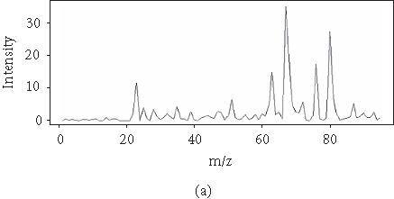
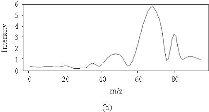
Original curve and a smoothed curve.

The next step performed on the smoothed curves is to find the landmarks or indices T_i. We collected the first derivative of ${\widehat{\mu }}_i\left(t\right)$, say ${\widehat{\mu }}_i^{\prime }\left(t\right)$, using a smoothing P-spline function available in R. Those derivatives are crucial at determining the cut-off points or indices of μ_i(t). We performed this step by computing an approximate 95% pointwise confidence interval for the first derivative of μ_i(t) [24]. When the lower limit of this interval is positive, we have the confidence that μ_i(t) will be increasing. When the upper limit of this interval is negative, we have the confidence that μ_i(t) will be decreasing. Inside the interval, when the derivative changes from negative to positive, we have an optimal value which is a minimum. When the derivative changes from positive to negative, we have an optimal value which is a maximum. The maximum is set, for convenience, as the largest value of ${\widehat{\mu }}_i^{\prime }\left(t\right)$ in that interval. In this study, we restricted the choice of indices to maximal values. Let ${\Lambda }_i=\left\{{\lambda }_1^{\left(i\right)},{\lambda }_2^{\left(i\right)},\dots ,{\lambda }_{m_i}^{\left(i\right)}\right\}$ be the collection of the estimated points where the curve μ_i(t) has a local maximum and let m_i be the number of maximals per observation or per sample (i). Consequently, dissimilarity measure is calculated to derive the dissimilarity matrices of size (n × n) for all samples using the maximum values.

Clustering spectral data using functional data analysis

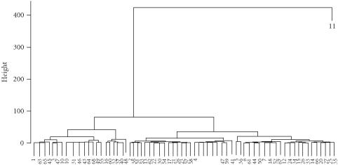
The application of functional data transformation led to the reduction of the dimensionality of the spectra to half. The size of mass indices become 12,598. To cluster the reduced data, we calculated the three dissimilarity matrices M_δC, M_δB, and M_δHZ. It appears that an unusual sample (patient 11) hides a possible pattern that we are trying to discover. Figure 3 shows a clustering dendrogram of the data using Diana approach. Pam and Clara gave the same results. This suggests that sample 11 would be important for further investigation.

Figure 3.

Clustering proteomics data with Diana.

When we removed observation 11, we detected a fewer fuzzy patterns with δ_C (Figure 4), δ_HZ (Figure 5), and δ_B (Figure 6). To be more specific, we investigated clusters proposed by δ_C and δ_HZ. A large number of clusters were proposed by both approaches (about 10 clusters). This strange result might be caused by the monotonicity assumption when using δ_HZ or the loss of information when using δ_C.

Figure 4.

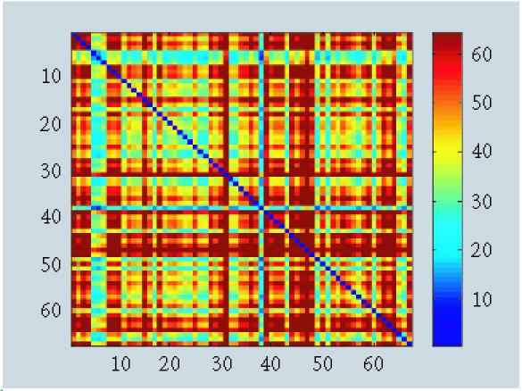
Pattern recognition using dissimilarity matrix δ_C.

Figure 5.

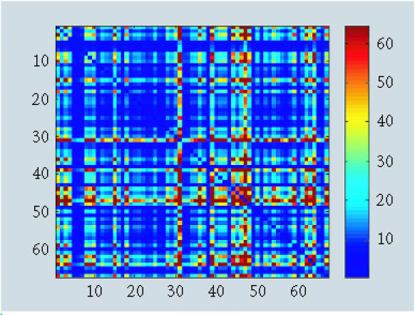
Pattern recognition using δ_HZ.

Figure 6.

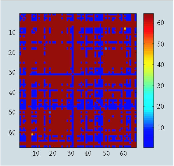
Pattern recognition using δ_B.

For δ_B, we provided the dendogram of the data using Diana approach (Figure 7). Three clusters were apparent. One well-separated cluster and two overlapped ones. For δ_HZ and δ_C, no structure was apparent which confirms the limitations of both dissimilarities as explained before.

Figure 7.

Dendogram of the δ_B dissimilarity approach with Diana.

To check the performance of our method, we calculated the confusion matrix between the predicted clusters and the clinical clusters using Diana (Table 1) and Clara (Table 2). We find that 3 patients out of 11 were misclassified for cluster 1 (HAM), 6 out of 20 were misclassified for cluster 2 (ATL), and 3 out of 37 were misclassified for cluster 3 (normal). Ham and ATL shared the majority of the misclassified observations which makes sense since both groups gather patients with a disease caused by the same retrospective virus. The error rate of misclassification for both clusters (HAM and ATL) is about 20%. For normal patient, the error rate of misclassification is about 8%. The total rate of misclassification is about 16%.

Table 1.

Confusion matrix to show the performance of δ_B using Diana.

	Predicted
	Classification	HAM	ATL	NOR	Total
Clinical	HAM	8	3	0	11
	ATL	5	14	1	20
	NOR	1	2	34	37
	Classification rate	0.73	0.70	0.92	0.84

Table 2.

Confusion matrix to show the performance of δ_B using Clara.

	Predicted
	Classification	HAM	ATL	NOR	Total
Clinical	HAM	10	1	0	11
	ATL	2	18	0	20
	NOR	1	1	35	37
	Classification rate	0.91	0.90	0.95	0.93

When we used Clara-based hierarchical cluster algorithm with δ_B, the classification result has dramatically been improved (Figure 8). The error rate of misclassification is reduced to 7%. The error rate of misclassification between HAM and ATL is about 9%, 5% of normal patients was misclassified. This result shows that a hierarchical δ_B dissimilarity algorithm based on minimizing the dissimilarity of observations to their closest medoid performs better than a divisive hierarchical clustering algorithm based on δ_B.

Figure 8.

The δ_B dissimilarity approach with Clara.

DISCUSSION

Cancer biomarkers can be used to screen asymptomatic individuals in the population, assist diagnosis in suspected cases, predict prognosis and response to specific treatments, and monitor patients after primary therapy. The introduction of new technologies to the proteome analysis field, such as mass spectrometry, have sparked new interest in cancer biomarkers allowing for more effective diagnosis of cancer by using complex proteomic patterns or for better classification of cancers, based on molecular signatures, respectively. These technologies provide wealth of information and rapidly generate large quantities of data.

Processing the large amounts of data will lead to useful predictive mathematical descriptions of biological systems which will permit rapid identification of novel therapeutic targets and diseases biomarkers.

Clustering and analyzing proteomics data has been proven to be a challenging task.

Proteomics data are provided usually as curves or spectra with thousand of peaks. A clustering algorithm based on a matrix of n observations (n samples which is usually small) and p peaks (p variables which is usually a large number) will be unsuccessful. A matrix of size (n ≪ p) will be singular and any method based on a matrix M (n × p) will not be robust enough and will induce errors. A clustering algorithm based on a well-chosen dissimilarity matrix (n × n) is more appropriate and more robust given the relatively moderate size of the matrix.

The use of a smoothing function for the spectra performs better for time series or for monotonic curves. We have previously successfully applied this smoothing function to large-scale proteomics data [25].

The application of Euclidean or Mahalanobis distances for instance may not perform well for this proteomics dataset, since those distances usually successfully applied to a typical data with specific expression, spherical or ellipsoidal (normally distributed data). A new dissimilarity measure has to involve other criteria such as the wealth of data points for each observation and the parallel nature expressed by the proteomics curve (or time series). On the other hand, a robust dissimilarity measure may perform badly on a curve with large data points or peaks.

Functional smoothing of proteomics expression profiles or spectra has proven to be very helpful. This has allowed us to minimize the number of peaks to retain only the ones that passed the performance of the FDA smoothing. In this study, after using FDA, we succeeded in retaining 50% of the smoothed peaks. The FDA with the dissimilarity measure δ_B shows better performance by comparison to δ_C and δ_HZ known to perform well along with FDA on times-series data or on monotonic curves.

The two remaining difficulties that naturally arose are (1) to find meaningful peaks that can be used to provide better discrimination between the clusters, (2) to propose the optimal number of clusters instead of choosing them a priori. The model selection criteria might be useful to answer those questions. In fact, model selection scores use two components for selecting the number of variables and the number of clusters in a given density-based cluster analysis. The first term is the lack of fit generally proportional to the likelihood function. The second term is the penalty term (complexity term). For such proteomics dataset, we propose to use the sum of the negative δ_B dissimilarity measure between all the observations to their closest medoids as a lack of fit function. The penalty term might be simple to derive but biased using AIC and BIC, for example, or it can be more difficult to derive if one used a more robust method such as information complexity-based criteria.

References

- 1.Aebersold R, Mann M. Mass spectrometry-based proteomics. Nature. 2003;422(6928):198–207. doi: 10.1038/nature01511. [DOI] [PubMed] [Google Scholar]
- 2.Steen H, Mann M. The ABC's (and XYZ's) of peptide sequencing. Nat Rev Mol Cell Biol. 2004;5(9):699–711. doi: 10.1038/nrm1468. [DOI] [PubMed] [Google Scholar]
- 3.Wright Jr G.L. SELDI proteinchip MS: a platform for biomarker discovery and cancer diagnosis. Expert Rev Mol Diagn. 2002;2(6):549–563. doi: 10.1586/14737159.2.6.549. [DOI] [PubMed] [Google Scholar]
- 4.Reddy G, Dalmasso E.A. SELDI protein chip(R) array technology: protein-based predictive medicine and drug discovery applications. J Biomed Biotechnol. 2003;2003(4):237–241. doi: 10.1155/S1110724303210020. [DOI] [PMC free article] [PubMed] [Google Scholar]
- 5.Tang N, Tornatore P, Weinberger S.R. Current developments in SELDI affinity technology. Mass Spectrom Rev. 2004;23(1):34–44. doi: 10.1002/mas.10066. [DOI] [PubMed] [Google Scholar]
- 6.Espina V, Mehta A.I, Winters M.E, et al. Protein microarrays: molecular profiling technologies for clinical specimens. Proteomics. 2003;3(11):2091–2100. doi: 10.1002/pmic.200300592. [DOI] [PubMed] [Google Scholar]
- 7.Zhang H, Yan W, Aebersold R. Chemical probes and tandem mass spectrometry: a strategy for the quantitative analysis of proteomes and subproteomes. Curr Opin Chem Biol. 2004;8(1):66–75. doi: 10.1016/j.cbpa.2003.12.001. [DOI] [PubMed] [Google Scholar]
- 8.Vazquez A, Flammini A, Maritan A, Vespignani A. Global protein function prediction from protein-protein interaction networks. Nat Biotechnol. 2003;21(1):697–700. doi: 10.1038/nbt825. [DOI] [PubMed] [Google Scholar]
- 9.Bensmail H, Haoudi A. Postgenomics: proteomics and bioinformatics in cancer research. J Biomed Biotechnol. 2003;2003(4):217–230. doi: 10.1155/S1110724303209207. [DOI] [PMC free article] [PubMed] [Google Scholar]
- 10.Somorjai R.L, Dolenko B, Baumgartner R. Class prediction and discovery using gene microarray and proteomics mass spectroscopy data: curses, caveats, cautions. Bioinformatics. 2003;19(12):1484–1491. doi: 10.1093/bioinformatics/btg182. [DOI] [PubMed] [Google Scholar]
- 11.Schwartz S.A, Weil R.J, Johnson M.D, Toms S.A, Caprioli R.M. Protein profiling in brain tumors using mass spectrometry: feasibility of a new technique for the analysis of protein expression. Clin Cancer Res. 2004;10(3):981–987. doi: 10.1158/1078-0432.ccr-0927-3. [DOI] [PubMed] [Google Scholar]
- 12.Ramsay J.O, Silverman B.W. Functional Data Analysis. New York, NY: Springer; 1997. [Google Scholar]
- 13.Ramsay J.O, Silverman B.W. Applied Functional Data Analysis: Methods and Case Studies. New York, NY: Springer; 2002. [Google Scholar]
- 14.Haoudi A, Semmes O.J. The HTLV-1 tax oncoprotein attenuates DNA damage induced G1 arrest and enhances apoptosis in p53 null cells. Virology. 2003;305(2):229–239. doi: 10.1006/viro.2002.1642. [DOI] [PubMed] [Google Scholar]
- 15.Haoudi A, Daniels R.C, Wong E, Kupfer G, Semmes O.J. Human T-cell leukemia virus-I tax oncoprotein functionally targets a subnuclear complex involved in cellular DNA damage-response. J Biol Chem. 2003;278(39):37736–37744. doi: 10.1074/jbc.M301649200. [DOI] [PubMed] [Google Scholar]
- 16.Adam B.L, Qu Y, Davis J.W, et al. Serum protein fingerprinting coupled with a pattern-matching algorithm distinguishes prostate cancer from benign prostate hyperplasia and healthy men. Cancer Res. 2002;62(13):3609–3614. [PubMed] [Google Scholar]
- 17.Piccolo D. A distance measure for classifying ARIMA models. Journal of Time Series Analysis. 1990;11:153–164. [Google Scholar]
- 18.Corduas M. La metrica autoregressiva tra modelli ARIMA: una procedura in linguaggio GAUSS. Quaderni di statistica. 2000;2:1–37. [Google Scholar]
- 19.Heckman N, Zamar R. Comparing the shapes of regression function. Biometrika. 2000;87(1):135–144. [Google Scholar]
- 20.Cerioli A, Laurini F, Corbellini A, editors. Functional cluster analysis of financial time series. In: Proceedings of the Meeting of Classification and Data Analysis Group of the Italian Statistical Society (CLADAG 2003); Bologna, Italy: CLUEB. 2003. pp. 107–110. [Google Scholar]
- 21.Ingrassia S, Cerioli A, Corbellini A. Some issues on clustering of functional data. In: Schader M, Gaul W, Vichi M, editors. Between Data Science and Applied Data Analysis. Berlin, Germany: Springer; 2003. pp. 49–56. [Google Scholar]
- 22.Kaufman L, Rousseeuw P.J. Finding Groups in Data. An Introduction to Cluster Analysis. New York, NY: John Wiley & Sons; 1990. [Google Scholar]
- 23.Hastie T.J, Tibshirani R.J. Generalized Additive Models. London UK: Chapman & Hall; 1990. [Google Scholar]
- 24.Silverman B.W. Some aspects of the spline smoothing approach to nonparametric regression curve fitting. J Roy Statist Soc B. 1985;47:1–52. [Google Scholar]
- 25.Bensmail H, Semmens J, Haoudi A. Bayesian fast-Fourier transform based clustering method for proteomics data. Journal of Bioinformatics. doi: 10.1093/bioinformatics/bti383. In press. [DOI] [PubMed] [Google Scholar]