Gene Expression Data Classification With Kernel Principal Component Analysis

Abstract

One important feature of the gene expression data is that the number of genes M far exceeds the number of samples N. Standard statistical methods do not work well when N < M. Development of new methodologies or modification of existing methodologies is needed for the analysis of the microarray data. In this paper, we propose a novel analysis procedure for classifying the gene expression data. This procedure involves dimension reduction using kernel principal component analysis (KPCA) and classification with logistic regression (discrimination). KPCA is a generalization and nonlinear version of principal component analysis. The proposed algorithm was applied to five different gene expression datasets involving human tumor samples. Comparison with other popular classification methods such as support vector machines and neural networks shows that our algorithm is very promising in classifying gene expression data.

INTRODUCTION

One important application of gene expression data is the classification of samples into different categories, such as the types of tumor. Gene expression data are characterized by many variables on only a few observations. It has been observed that although there are thousands of genes for each observation, a few underlying gene components may account for much of the data variation. Principal component analysis (PCA) provides an efficient way to find these underlying gene components and reduce the input dimensions (Bicciato et al [1]). This linear transformation has been widely used in gene expression data analysis and compression (Bicciato et al [1], Yeung and Ruzzo [2]). If the data are concentrated in a linear subspace, PCA provides a way to compress data and simplify the representation without losing much information. However, if the data are concentrated in a nonlinear subspace, PCA will fail to work well. In this case, one may need to consider kernal principal component analysis (KPCA) (Rosipal and Trejo [3]). KPCA is a nonlinear version of PCA. It has been studied intensively in the last several years in the field of machine learning and has claimed success in many applications (Ng et al [4]). In this paper, we introduce a novel algorithm of classification, based on KPCA. Computational results show that our algorithm is effective in classifying gene expression data.

ALGORITHM

A gene expression dataset with M genes (features) and N mRNA samples (observations) can be conveniently represented by the following gene expression matrix:

$$X=\left[\begin{array}{cccc}{x}_{11}& x_{12}& \cdots & x_{1N}\\ x_{21}& x_{22}& \dots & x_{2N}\\ ⋮& ⋮& \ddots & ⋮\\ x_{M1}& x_{M2}& \cdots & x_{MN}\end{array}\right],\left(1\right)$$

where x_li is the measurement of the expression level of gene l in mRNA sample i. Let x_i = (x_1i, x_2i, ..., x_Mi)′ denote the ith column (sample) of X with the prime ′ representing the transpose operation, and y_i the corresponding class label (eg, tumor type or clinical outcome).

KPCA is a nonlinear version of PCA. To perform KPCA, one first transforms the input data x from the original input space F₀ into a higher-dimensional feature space F₁ with the nonlinear transform x → Φ(x), where Φ is a nonlinear function. Then a kernel matrix K is formed using the inner products of new feature vectors. Finally, a PCA is performed on the centralized K, which is the estimate of the covariance matrix of the new feature vector in F₁. Such a linear PCA on K may be viewed as a nonlinear PCA on the original data. This property is sometimes called “kernel trick” in the literature. The concept of kernel is very important, here is a simple example to illustrate it. Suppose we have a two-dimensional input x = (x₁, x₂)′, let the nonlinear transform be

$$\mathbf{x}\to \Phi \left(\mathbf{x}\right)={\left(x_1^2,x_2^2,\sqrt{2}{x}_1{x}_2,\sqrt{2}{x}_1,\sqrt{2}{x}_2,1\right)}^{\prime }.\left(2\right)$$

Therefore, given two points x_i = (x_i1, x_i2)′ and x_j = ( x_j1, x_j2)′, the inner product (kernel) is

$$\begin{array}{l}K\left({\mathbf{x}}_i,{\mathbf{x}}_j\right)=\Phi {\left({\mathbf{x}}_i\right)}^{\prime }\Phi \left({\mathbf{x}}_j\right)\\ =x_{i1}^2{x}_{j1}^2+x_{i2}^2{x}_{j2}^2+2x_{i1}{x}_{i2}{x}_{j1}{x}_{j2}\\ +2x_{i1}{x}_{j1}+2x_{i2}{x}_{j2}+1\\ ={\left(1+x_{i1}{x}_{j1}+x_{i2}{x}_{j2}\right)}^2={\left(1+{{\mathbf{x}}^{\prime }}_i{\mathbf{x}}_j\right)}^2,\end{array}\left(3\right)$$

which is a second-order polynomial kernel. Equation (3) clearly shows that the kernel function is an inner product in the feature space and the inner products can be evaluated without even explicitly constructing the feature vector Φ(x).

The following are among the popular kernel functions:

1. first norm exponential kernel

   $$K\left({\mathbf{x}}_i,{\mathbf{x}}_j\right)=exp\left(-\beta \Vert {\mathbf{x}}_i-{\mathbf{x}}_j\Vert \right),\left(4\right)$$
2. radial basis function (RBF) kernel

   $$K\left({\mathbf{x}}_i,{\mathbf{x}}_j\right)=exp\left(-\frac{{\left|{\mathbf{x}}_i-{\mathbf{x}}_j\right|}^2}{{\sigma }^2}\right),\left(5\right)$$
3. power exponential kernel (a generalization of RBF kernel)

   $$K\left({\mathbf{x}}_i,{\mathbf{x}}_j\right)=exp\left[-{\left(\frac{{\left|{\mathbf{x}}_i-{\mathbf{x}}_j\right|}^2}{r^2}\right)}^{\beta }\right],\left(6\right)$$
4. sigmoid kernel

   $$K\left({\mathbf{x}}_i,{\mathbf{x}}_j\right)=tanh\left(\beta {{\mathbf{x}}^{\prime }}_i{\mathbf{x}}_j\right),\left(7\right)$$
5. polynomial kernel

   $$K\left({\mathbf{x}}_i,{\mathbf{x}}_j\right)={\left({{\mathbf{x}}^{\prime }}_i{\mathbf{x}}_j+p_2\right)}^{p1},\left(8\right)$$

   where p₁ and p₂ = 0, 1, 2, 3,... are both integers.

For binary classification, our algorithm, based on KPCA, is stated as follows.

KPC classification algorithm

Given a training dataset ${\left\{{\mathbf{x}}_i\right\}}_{i=1}^n$ with class labels ${\left\{y_i\right\}}_{i=1}^n$ and a test dataset ${\left\{{\mathbf{x}}_t\right\}}_{t=1}^{n_t}$ with labels ${\left\{y_t\right\}}_{t=1}^{n_t}$, do the following.

1. Compute the kernel matrix, for the training data, K = [K_ij]_n×n, where K_ij = K(x_i, x_j). Compute the kernel matrix, for the test data, K_te = [K_ti]_{nt × n}, where K_ti = K(x_t, x_i). K_ti projects the test data x_t onto training data x_i in the high-dimensional feature space in terms of the inner product.

2. Centralize K using and K_te

   $$\begin{array}{l}K=\left({\mathbf{I}}_n-\frac{1}{n}{\mathbf{1}}_n{{\mathbf{1}}^{\prime }}_n\right)K\left({\mathbf{I}}_n-\frac{1}{n}{\mathbf{1}}_n{{\mathbf{1}}^{\prime }}_n\right),\\ K_{\text{te}}=\left(K_{\text{te}}-\frac{1}{n}{\mathbf{1}}_{n_t}{{\mathbf{1}}^{\prime }}_{n}K\right)\left(\mathbf{I}-\frac{1}{n}{\mathbf{1}}_n{{\mathbf{1}}^{\prime }}_n\right).\end{array}\left(9\right)$$

3. Form an n × k matrix Z =[z₁ z₂ ... z_k], where z₁, z₂, ..., z_k are eigenvectors of K that correspond to the largest eigenvalues λ₁ ≥ λ₂ ≥ ... ≥ λ_k > 0. Also form a diagonal matrix D with λ_i in a position (i, i).

4. Find the projections V= KZD^−1/2 and V_te = K_te ZD^−1/2 for the training and test data, respectively.

5. Build a logistic regression model using V and ${\left\{y_i\right\}}_{i=1}^n$ and test the model performance using V_te and ${\left\{y_t\right\}}_{t=1}^{n_t}$.

We can show that the above KPC classification algorithm is a nonlinear version of the logistic regression. From our KPC classification algorithm, the probability of the label y, given the projection v, is expressed as

$$P\left(y|\mathbf{w},\mathbf{v}\right)=g\left(b+\sum _{i=1}^k{w}_i{v}_i\right),\left(10\right)$$

where the coefficients w are adjustable parameters and g is the logistic function

$$g\left(u\right)={\left(1+exp\left(-u\right)\right)}^{-1}.\left(11\right)$$

Let n be the number of training samples and Φ the nonlinear transform function. We know each eigenvector z_i lies in the span of Φ(x₁), Φ(x₂), ..., Φ(x_n) for i = 1, ..., n (Rosipal and Trejo [3]). Therefore one can write, for constants z_ij,

$$z_i=z_{i1}\Phi \left({\mathbf{x}}_1\right)+z_{i2}\Phi \left({\mathbf{x}}_2\right)+\dots +z_{in}\Phi \left({\mathbf{x}}_n\right)=\sum _{j=1}^n{z}_{ij}\Phi \left({\mathbf{x}}_j\right).\left(12\right)$$

Given a test data x, let v_i denote the projection of Φ(x) onto the ith nonlinear component with a normalizing factor $1/\sqrt{{\lambda }_i}$, we have

$$v_i=\frac{1}{\sqrt{{\lambda }_i}}\left({z^{\prime }}_i\Phi \left(\mathbf{x}\right)\right)=\frac{1}{\sqrt{{\lambda }_i}}\sum _{j=1}^n{z}_{ij}K\left({\mathbf{x}}_j,\mathbf{x}\right).\left(13\right)$$

Substituting (13) into (10), we have

$$P\left(y|\mathbf{w},\mathbf{v}\right)=g\left(b+\sum _{j=1}^n{c}_{j}K\left({\mathbf{x}}_j,\mathbf{x}\right)\right),\left(14\right)$$

where

$$c_j=\sum _{i=1}^k\frac{1}{\sqrt{{\lambda }_i}}{w}_i{z}_{ij},\hspace{0.17em}\hspace{0.17em}\hspace{0.17em}\hspace{0.17em}i=1,\dots ,n.\left(15\right)$$

When K(x_i, x_j) = x_i′x _j, (14) becomes logistic regression. K(x_i, x_j) = x_i′x_j is a linear kernel (polynomial kernel with p₁ = 1 and p₂ = 0). When we first normalize the input data through minusing their mean and then dividing their standard deviation, linear kernel matrix is the covariance matrix of the input data. Therefore KPC classification algorithm is a generalization of logistic regression.

Described in terms of binary classification, our classification algorithm can be readily employed for multiclass classification tasks. Typically, two-class problems tend to be much easier to learn than multiclass problems. While for two-class problems only one decision boundary must be inferred, the general c-class setting requires us to apply a strategy for coupling decision rules. For a c-class problem, we employ the standard approach where two-class classifiers are trained in order to separate each of the classes against all others. The decision rules are then coupled by voting, that is, sending the sample to the class with the largest probability.

Mathematically, we build c two-class classifiers based on a KPC classification algorithm in the form of (14) with the scheme “one against the rest”:

$$p_i=P\left(y=i|\mathbf{x}\right)=g\left(b_i+\sum _{i=1}^n{w}_{ij}K\left({\mathbf{x}}_i,\mathbf{x}\right)\right),\left(16\right)$$

where i =1, 2, ..., c. Then for a test data point x_t, we have the predicted class

$${\hat{y}}_t=\underset{i=1,\dots ,c}{argmax}{p}_i\left({\mathbf{x}}_t\right).\left(17\right)$$

Feature and model selections

Since many genes show little variation across samples, gene (feature) selection is required. We chose the most informative genes with the highest likelihood ratio scores, described below (Ideker et al [5]). Given a two-class problem with an expression matrix X = [x_li]_{M × N}, we have, for each gene l,

$$T\left(x_l\right)=log\frac{{\sigma }^2}{{{\sigma }^{\prime }}^2},\left(18\right)$$

where

$$\begin{array}{l}{\sigma }^2=\sum _{i=1}^N{\left(x_{li}-\mu \right)}^2,\\ {{\sigma }^{\prime }}^2=\sum _{i\in \text{class}0}{\left(x_{li}-{\mu }_0\right)}^2+\sum _{i\in \text{class}1}{\left(x_{li}-{\mu }_1\right)}^2.\end{array}\left(19\right)$$

Here μ, μ₀, and μ₁ are the whole sample mean, the Class 0 mean, and the Class 1 mean, alternatively. We selected the most informative genes with the largest T values. This selection procedure is based on the likelihood ratio and used in our classification.

On the other hand, the dimension of projection (the number of eigenvectors) k used in the model can be selected based on Akaike's information criteria (AIC):

$$\text{AIC}=-2log\left(\hat{L}\right)+2\left(k+1\right),\left(20\right)$$

where $\hat{L}$ is the maximum likelihood and k is the dimension of the projection in (10). The maximum likelihood $\hat{L}$ can also be calculated using (10):

$$\hat{L}=\prod _{i=1}^n{\left(p\left(y|\mathbf{w},\mathbf{v}\right)\right)}^y{\left(1-p\left(y|\mathbf{w},\mathbf{v}\right)\right)}^{1-y}.\left(21\right)$$

We can choose the best k with minimum AIC value.

COMPUTATIONAL RESULTS

To illustrate the applications of the algorithm proposed in the previous section, we considered five gene expression datasets: leukemia (Golub et al [6]), colon (Alon et al [7]), lung cancer (Garber et al [8]), lymphoma (Alizadeh et al [9]), and NCI (Ross et al [10]). The classification performance is assessed using the “leave-one-out (LOO) cross validation” for all of the datasets except for leukemia which uses one training and test data only. LOO cross validation provides more realistic assessment of classifiers which generalize well to unseen data. For presentation clarity, we give the number of errors with LOO in all of the figures and tables.

Leukemia

The leukemia dataset consists of expression profiles of 7129 genes from 38 training samples (27 ALL and 11 AML) and 34 testing samples (20 ALL and 14 AML). For classification of leukemia using a KPC classification algorithm, we chose the polynomial kernel K(x_i, x_j) = (x_i′x_j + 1)² and 15 eigenvectors corresponding to the first 15 largest eigenvalues with AIC. Using 150 informative genes, we obtained 0 training error and 1 test error. This is the best result compared with those reported in the literature. The plot for the output of the test data is given in Figure 1, which shows that all the test data points are classified correctly except for the last data point.

Figure 1.

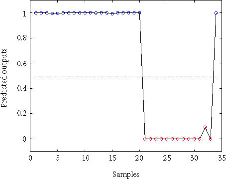
Output of the test data with KPC classification algorithm.

Colon

The colon dataset consists of expression profiles of 2000 genes from 22 normal tissues and 40 tumor samples. We calculated the classification result using a KPC classification algorithm with a kernel K(x_i, x_j) = (x_i′x_j + 1)². There were 150 selected genes and 25 eigenvectors selected with AIC criteria. The result is compared with that from the linear principal component (PC) logistic regression. The classification errors were calculated with the LOO method. The average error with linear PC logistic regression is 2 and the error with KPC classification is 0. The detailed results are given in Figure 2.

Figure 2.

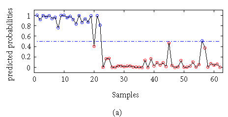
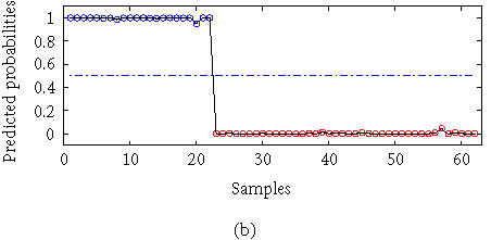
Outputs with (a) linear PC regression and (b) KPC classification.

Lung cancer

The lung cancer dataset has 918 genes, 73 samples, and 7 classes. The number of samples per class for this dataset is small (less than 10) and unevenly distributed with 7 classes, which makes the classification task more challenging. A third-order polynomial kernel K(x_i, x_j) = (x_i′x_j +1)³, and an RBF kernel with σ = 1 were used in the experiments. We chose the 100 most informative genes and 20 eigenvectors with our gene and model selection methods. The computational results of KPC classification and other methods are shown in Table 1. The results from SVMs for lung cancer, lymphoma, and NCI shown in this paper are those from Ding and Peng [11]. Six misclassifications with KPC and a polynomial kernel are given in Table 2. Table 1 shows that KPC with a polynomial kernel is performed better than that with an RBF kernel.

Table 1.

Comparison for lung cancer.

Methods	Number of errors
KPC with a polynomial kernel	6
KPC with an RBF kernel	8
Linear PC classification	7
SVMs	7
Regularized logistic regression	12

Table 2.

Misclassifications of lung cancer.

Sample index	True class	Predicted class
6	6	4
12	6	4
41	6	3
51	3	6
68	1	5
71	4	3

Lymphoma

The lymphoma dataset has 4026 genes, 96 samples, and 9 classes. A third-order polynomial kernel K(x_i, x_j) = (x_i′x_j + 1)³ and an RBF kernel with σ = 1 were used in our analysis. The 300 most informative genes and 21 eigenvectors corresponding to the largest eigenvalues were selected with the gene selection method and AIC criteria. A comparison of KPC with other methods is shown in Table 3. Misclassifications of lymphoma using KPC with a polynomial kernel are given in Table 4. There are only 2 misclassifications of class 1 using our KPC algorithm with a polynomial kernel, as shown in Table 4. The KPC with a polynomial kernel outperformed that with an RBF kernel in this experiment.

Table 3.

Comparison for lymphoma.

Methods	Number of errors
KPC with a polynomial kernel	2
KPC with an RBF kernel	6
PC	5
SVMs	2
Regularized logistic regression	5

Table 4.

Misclassifications of lymphoma.

Sample index	True class	Predicted class
64	1	6
96	1	3

NCI

The NCI dataset has 9703 genes, 60 samples, and 9 classes. The third-order polynomial kernel K(x_i, x_j) = (x_i′x_j + 1)³ and an RBF kernel with σ = 1 were chosen in this experiment. The 300 most informative genes and 23 eigenvectors were selected with our simple gene selection method and AIC criteria. A comparison of computational results is summarized in Table 5 and the details of misclassification are listed in Table 6. KPC classification has equivalent performance with other popular tools.

Table 5.

Comparison for NCI.

Methods	Number of errors
KPC with a polynomial kernel	6
KPC with a RBF kernel	7
PC	6
SVMs	12
Logistic regression	6

Table 6.

Misclassifications of NCI.

Sample index	True class	Predicted class
6	1	3
7	1	4
27	4	3
45	7	9
56	8	5
58	8	1

DISCUSSIONS

We have introduced a nonlinear method, based on kPCA, for classifying gene expression data. The algorithm involves nonlinear transformation, dimension reduction, and logistic classification. We have illustrated the effectiveness of the algorithm in real life tumor classifications. Computational results show that the procedure is able to distinguish different classes with high accuracy. Our experiments also show that KPC classifications with second- and third-order polynomial kernels are usually performed better than that with an RBF kernel. This phenomena may be explained from the special structure of gene expression data. Our future work will focus on providing a rigorous theory for the algorithm and exploring the theoretical foundation that KPC with a polynomial kernel performed better than that with other kernels.

DISCLAIMER

The opinions expressed herein are those of the authors and do not necessarily represent those of the Uniformed Services University of the Health Sciences and the Department of Defense.

References

- 1.Bicciato S, Luchini A, Di Bello C. PCA disjoint models for multiclass cancer analysis using gene expression data. Bioinformatics. 2003;19(5):571–578. doi: 10.1093/bioinformatics/btg051. [DOI] [PubMed] [Google Scholar]
- 2.Yeung K.Y, Ruzzo W.L. Principal component analysis for clustering gene expression data. Bioinformatics. 2001;17(9):763–774. doi: 10.1093/bioinformatics/17.9.763. [DOI] [PubMed] [Google Scholar]
- 3.Rosipal R, Trejo L.J. Tech. Rep. London: University of Paisley; 2001. Mar, Kernel partial least squares regression in RKHS: theory and empirical comparison. [Google Scholar]
- 4.Ng A, Jordan M, Weiss Y, editors. On spectral clustering: Analysis and an algorithm. In: Advances in Neural Information Processing Systems 14, Proceedings of the 2001; Vancouver, British Columbia: MIT Press; 2001. pp. 849–856. [Google Scholar]
- 5.Ideker T, Thorsson V, Siegel A.F, Hood L.E. Testing for differentially-expressed genes by maximum-likelihood analysis of microarray data. J Comput Biol. 2000;7(6):805–817. doi: 10.1089/10665270050514945. [DOI] [PubMed] [Google Scholar]
- 6.Golub T.R, Slonim D.K, Tamayo P, et al. Molecular classification of cancer: class discovery and class prediction by gene expression monitoring. Science. 1999;286(4539):531–537. doi: 10.1126/science.286.5439.531. [DOI] [PubMed] [Google Scholar]
- 7.Alon U, Barkai N, Notterman D.A, et al. Broad patterns of gene expression revealed by clustering analysis of tumor and normal colon tissues probed by oligonucleotide arrays. Proc Natl Acad Sci USA. 1999;96(12):6745–6750. doi: 10.1073/pnas.96.12.6745. [DOI] [PMC free article] [PubMed] [Google Scholar]
- 8.Garber M.E, Troyanskaya O.G, Schluens K, et al. Diversity of gene expression in adenocarcinoma of the lung. Proc Natl Acad Sci USA. 2001;98(24):13784–13789. doi: 10.1073/pnas.241500798. [DOI] [PMC free article] [PubMed] [Google Scholar]
- 9.Alizadeh A.A, Eisen M.B, Davis R.E, et al. Distinct types of diffuse large B-cell lymphoma identified by gene expression profiling. Nature. 2000;403(6769):503–511. doi: 10.1038/35000501. [DOI] [PubMed] [Google Scholar]
- 10.Ross D.T, Scherf U, Eisen M.B, et al. Systematic variation in gene expression patterns in human cancer cell lines. Nat Genet. 2000;24(3):227–235. doi: 10.1038/73432. [DOI] [PubMed] [Google Scholar]
- 11.Ding C, Peng H, editors. Minimum redundancy feature selection from microarray gene expression data. In: Proc IEEE Bioinformatics Conference (CSB '03); Berkeley, Calif: IEEE; 2003. pp. 523–528. [DOI] [PubMed] [Google Scholar]