A single-cell transcriptomic atlas of developing inhibitory neurons reveals expanding and contracting modes of diversification

Abstract

The cerebral cortex relies on vastly different types of inhibitory neurons to compute. How this diversity emerges during development remains an open question. The rarity of individual inhibitory neuron types often leads to their underrepresentation in single-cell RNA sequencing (scRNAseq) datasets, limiting insights into their developmental trajectories. To address this problem, we developed a computational pipeline to enrich and integrate rare cell types across multiple datasets. Applying this approach to somatostatin-expressing (SST+) inhibitory neurons—the most diverse inhibitory cell class in the cortex—we constructed the Dev-SST-Atlas, a comprehensive resource containing mouse transcriptomic data of over 51,000 SST+ neurons. We identify three principal groups—Martinotti cells (MCs), non-Martinotti cells (nMCs), and long-range projecting neurons (LRPs)—each following distinct diversification trajectories. MCs commit early, with distinct embryonic and neonatal clusters that map directly to adult counterparts. In contrast, nMCs diversify gradually, with each developmental cluster giving rise to multiple adult cell types. LRPs follow a unique ‘contracting’ mode. Initially, two clusters are present until postnatal day 5 (P5), but by P7, one type is eliminated through programmed cell death, leaving a single surviving population. This transient LRP type is also found in the fetal human cortex, revealing an evolutionarily conserved feature of cortical development. Together, these findings highlight three distinct modes of SST+ neuron diversification—invariant, expanding, and contracting—offering a new framework to understand how the large repertoire of inhibitory neurons emerges during development.

Introduction

Cortical inhibitory neurons orchestrate information processing, coordinate network synchrony and are essential to circuit homeostasis^1–7. Dysregulation in their development has been implicated in a range of neurological disorders^7–13, including epilepsy, schizophrenia, and autism. This underscores the critical need to understand how these neurons develop and diversify.

Advances in single-cell and single-nucleus RNA sequencing (sc/snRNA-seq) have transformed the study of brain tissue, which contains heterogeneous cell types. However, adequate representation of cortical inhibitory neurons in scRNAseq datasets remains particularly challenging due to their rarity and their diversity. Resolving their developmental trajectories requires either extensive enrichment or sequencing of large populations—approaches that are not standard in most experiments.

In the adult mouse cortex and hippocampus, inhibitory neurons make up only ~15% of cortical neurons, with the remaining ~85% being excitatory glutamatergic neurons^4,7,14. Within this minority population, SST+ neurons stand out due to their exceptionally high transcriptional and functional diversity^15–19, further contributing to poor representation of specific cell types. Recent efforts to construct large-scale single-cell atlases, such as the ABC Atlas^15,20, have introduced hierarchical classification systems—class, subclass, supertype, and type or clusters—that improve the granularity of cell type annotation. However, rare cell types remain severely underrepresented; for instance, 16% of SST+ types (or clusters) are represented by fewer than 150 cells, compared to only 2.7% of excitatory pyramidal neuron types^15,20. Similar underrepresentation persists in human brain scRNA-seq datasets, where rare inhibitory neuron types, such as Sst-Chodl neurons, are particularly sparse²¹.

The challenge of poor representation is further compounded in developmental datasets^22–26. During early development, transcriptional profiles are dominated by immature signatures, which obscure cellular diversity^22–26. For SST+ neurons—encompassing Martinotti cells (MCs), non-Martinotti cells (nMCs), and long-range projecting neurons (LRPs)^{4,6,7,23,26–30}—understanding developmental trajectories is particularly difficult due to the lack of fine-scale resolution in existing data.

To overcome these limitations, we developed a computational pipeline to enhance the detection and integration of rare neuronal cell types in developmental scRNA-seq datasets. Our computational pipeline consists of three modules: (i) rare cell extraction, (ii) dataset integrability assessment, and (iii) hierarchical clustering for atlas construction. Using SST+ neurons as a model system, we constructed Dev-SST-v1, a high-resolution developmental resource that spans embryonic day 16.5 (E16.5) to postnatal day 5 (P5). This atlas includes over 51,000 SST+ neurons, representing a seven-fold increase in sampling compared to our previous efforts²³.

Our analysis reveals three principal groups of SST+ neurons—Martinotti cells (MCs), non-Martinotti cells (nMCs), and long-range projecting neurons (LRPs)—each with distinct diversification and developmental trajectories. MCs follow an invariant trajectory, where early developmental clusters align closely with adult cell types, similar to excitatory pyramidal neurons³¹, Chandelier, and Meis2+ interneurons^22,32. nMCs exhibit an expanding trajectory, where a single neonatal cluster gives rise to multiple adult types, resembling retinal ganglion cell development³³. LRPs undergo a “contracting” trajectory, with two early postnatal clusters persisting until P5, after which one is selectively eliminated through programmed cell death, leaving a single surviving type in adulthood.

In summary, our computational pipeline is a powerful resource for studying rare neuronal cell types. Dev-SST-v1, the most comprehensive single cell inhibitory neuron atlas to date, revealed an unprecedented palette of cell diversification strategies in the developing mammalian cortex.

Results

Developing inhibitory neurons are poorly represented in most scRNAseq datasets.

Somatostatin-expressing (SST+) inhibitory neurons represent about 3–4% of all cortical neurons, and are one of the most diverse classes among inhibitory neurons^{7,15–17,19,34}. In adult mouse neocortex, scRNAseq datasets have shown that these inhibitory cells can be grouped into 19 supertypes and 45 to 73 types or clusters^15,17,20. To investigate the development of these rare neurons, we constructed a high-resolution, integrable single-cell atlas by extracting SST+ cells from multiple datasets. Our computational pipeline consists of three modules designed for this purpose (Fig. 1a).

Figure 1. Integrative scRNAseq developmental atlas for SST+ inhibitory neurons.

(a) Schematic of the three-step integrative pipeline for generating an atlas. Step 1: Selection of rare cell classes (SST+) from publicly available scRNAseq datasets. Step 2: Assessment of dataset integrability using anchor points, k-nearest-neighbor (k-NN) graph evaluation, and k-BET testing. Step 3: Construction of the new developmental SST+ atlas (Dev-SST-Atlas) by integrating accepted datasets, reclustering, and quality control, (b) Bar plot showing the distribution of SST+ cells identified in each dataset in Module 1, highlighting variability in SST+ cell representation across datasets, (c) UMAP visualization of Atlas-v0, comprising 19,874 SST+ cells, annotated by sample types, main groups, and subtype labels transferred from Fisher et al. (2024)²³. (d) UMAP embedding of Atlas-v0 reannotated using MapMyCells with ABC Atlas (Yao et al. 2023)¹⁵, overlaying mapping probabilities for each cell, (e) Stacked bar plot depicting the relative abundance of subclasses in Atlas-v0, restricted to cells with mapping high probabilities (>0.9).

In the first module (Module 1), we systematically survey publicly available scRNAseq datasets from the developing mouse cortex spanning embryonic day (E)12.5 to postnatal day (P)10 (Extended Data Table 1), collectively comprising more than 1.5 million cells^{23,26,35–49}. Initial quality control measures included filtering out cells with low counts and high mitochondrial DNA content (Methods; Extended Data Fig. 1a). SST+ cells were identified by clustering each dataset and selecting populations expressing both Sst and Lhx6, two key markers of developing inhibitory neurons^{7,24,27,50,51}.To exclude contaminating interneurons, we removed Meis2+ (SST-negative) cells known to appear in Sst^cre driver lines²³.

Of the 17 datasets analyzed (DS1–DS17^{23,26,35–49}), only six contained more than 1,000 SST+ neurons (Extended Data Table 1a, Fig. 1b). The largest dataset, from Fisher et al. (2024)²³, contained ~19,000 SST+ cells and was used to generate a preliminary reference, Atlas-v0, incorporating data from four experiments spanning three developmental stages (E16.5, P1, P5).

To annotate Atlas-v0, we performed label transfer using annotations from Fisher et al.²³ (Fig 1c). Then, we mapped developmental cells onto adult inhibitory neuron reference data from Yao et al. (2023)¹⁵, using the Allen Institute’s MapMyCells algorithm (RRID:SCR_024672). At the subclass level, more than 75% of Atlas-v0 cells aligned with adult SST+ inhibitory neurons (Sst 053, Sst-Chodl 056; Fig. 1d, 1e), with high confidence (>0.9 probability). Approximately 15% of cells mapped to Pvalb (052) or olfactory-striatal inhibitory neurons (045 OB-STR; Fig. 1e). Given that SST+ cells in Atlas-v0 were enriched using fluorescence-activated cell sorting (FACS) from Sst^cre;RCE animals, which contain minimal (<1%) Pvalb+ cells²³, this suggests that a subset of developing SST+ neurons may transcriptomically resemble adult Pvalb+ and olfactory-striatal interneurons. Overall, Module 1 of our computational pipeline selectively and accurately extracts rare cell types.

A generalized computational pipeline to assess integrability of different datasets.

The second module (Module 2) of our pipeline was designed to examine structural similarities between two distinct datasets (Fig. 1a, Extended Data Fig. 1b). Since only 6 datasets contain more than 1000 SST+ (Extended Data Table 1), we reasoned these small numbers of cells would not give us sufficient representation to build a high resolution atlas for SST+ neurons. Therefore, we generated 7 more datasets (DS18 to DS24, Extended Data Table 1), all containing more than 1000 SST+ cells from the developing mouse cortex from E16.5 to P5 (Fig. 2a). Most of these are enriched by FACS as previously described²³ (see methods). For these unpublished datasets, we applied the computational pipeline of Module 1 to extract all SST+ cells (Fig. 2a).

Figure 2. Computational pipeline to assess the integrability of different datasets.

(a) Tabular overview of datasets used to test integrability with Atlas-v0, including both newly generated and published datasets. The table lists SST+ cell counts, mean anchor points, k-BET (k-nearcst-ncighbor batch effect test) rejection rate, and fractions of cclls within Atlas-v0 neighborhoods (k = 75) for each dataset, (b) Bar plot of mean anchor points calculated using Seurat’s CCA integration function between each dataset and Atlas-v0. Datasets with >2000 mean anchor points (horizontal dashed line) were considered intcgrablc. (c) Fraction of cells in each dataset within Atlas-v0 neighborhoods with increasing k value. The dashed line (k = 75) indicates the acceptance threshold of >50%. (d, e) Dot plot of (d) fraction cells within k-NN (k—75) and (e) k-BET rejection plotted against anchor points rates for cach dataset. Datasets passing the three integrability criteria (in green) have mean anchor points >2000, fraction within k-NN >50%, and k-BET rejection rate <0.5.

Next, we proceeded to assess if the SST+ inhibitory neurons from different sources, both published and newly generated datasets, can be integrated using three distinct criteria. For the first criteria, we calculated the number of anchor points using the Seurat CCA integration function between the SST+ cells extracted from each dataset and Atlas-v0. As Atlas-v0 contains 4 distinct samples published by Fisher et al.²³, we calculated anchor points of each new dataset to each of the samples (see Methods). We set the criteria for acceptance as datasets with >2000 mean anchor points (Fig. 2a, 2b).

For the second criteria, we determined the k-nearest neighbor (k-NN) in each dataset using principal components computed on the integrated counts matrix. Then, we evaluated the neighborhood composition for all the cells in each dataset, and determined the percentage of cells that have similar neighborhoods (k-NN), which is 50% in Atlas-v0. By adjusting the neighborhood size (k from 0 to 200), we estimated the structure similarly of each dataset to Atlas-v0 (Fig. 2c). We set the acceptance criteria for each dataset as having >50% of cells within the same k-NN (k=75), as observed in Atlas-v0 (Fig. 2d).

For the last criterion, we calculated the k-BET rejection rate⁵², a test commonly used for assessing samples similarly from different batches. We set the acceptance criteria as k-BET < 0.5 (Fig. 2a, 2e). Among the 13 datasets subjected to these tests (Fig. 2a, 2d, 2e), 7 datasets passed all three criteria and they were used to generate a developmental atlas for SST+ neurons in Module 3.

The parameters measured in Module 2 are generalizable, and can be applied to other datasets to assess integrability across different experimental conditions (Extended Data Fig. 2a). As an example, we took unpublished snRNAseq datasets generated from 13 samples of mouse adult spinal cords, representing different experimental conditions from Aya Takeoka’s laboratory. One control sample was used as the “reference/base atlas”, akin to our Atlas-v0, and the integrability of subsequent biological samples were assessed using this reference sample. Even though cellular diversity, ages, and sample types were different, Module 2 can be used to assess integrability by computing the three criteria: mean anchor point (Extended Data Fig. 2a, 2c), fraction within k-NN (Extended Data Fig. 2a, 2b, 2d), and k-BET rejection rate (Extended Data Fig. 2a, 2e).

Integrability criteria do not depend on sequencing depth

To identify factors that influence integrability of independent datasets, we searched for dataset-specific features in experimental setup and computational analyses. Since all datasets were subjected to the same QC parameters in Module 1 (read counts, ribosomal RNA, mitochondria genes), cellular heterogeneity and general quality of transcripts within each dataset are unlikely to be the separating factors. We noted that sequencing read depth differs greatly between laboratories and samples, and thus examined whether this could be a potential factor.

To this end, we took two datasets that we generated (DS21 and DS24) from two stages, E16.5 and P1, and performed both shallow and deep sequencing on the same samples. For shallow sequencing, we targeted a sequencing depth of 5000 reads per cell; the actual mean reads achieved was 8,227 +/− 794. For deep sequencing, we targeted 50,000 reads per cell; the actual mean reads achieved was 61,384 +/− 20,484 (Fig. 3a). Then, we performed the integrability test (Module 2) by quantifying the 3 parameters: anchor points with Atlas-v0, fraction of cells within k-NN, and the k-BET rejection test (Fig. 3b–3e).

Figure 3. Integrability of the same dataset with variations in sequencing depth.

(a) Comparison of sequencing depth between shallow and deep sequencing datasets DS21 and DS24. Shallow sequencing targeted 5,000 reads per cell (mean achieved: 8,227 ± 794 reads per cell), while deep sequencing targeted 50,000 reads per cell (mean achieved: 61,384 ± 20,484 reads per cell), (b) Mean anchor points for DS21 and DS24 under shallow (S) and deep sequencing protocols. While DS21-S showed a slight reduction in anchor points below the acceptance threshold of 2,000 (horizontal dashed line), DS24-S maintained integrability. (c) Fraction of cells in shallow- and deep-sequenced datasets within Atlas-v0 neighborhoods with increasing k value. Both shallow and deep sequencing protocols met the acceptance threshold of >50% (k=75) (dashed line), (d, e) Dot plot of (d) fraction cells within k-NN (k-75) and (e) k-BET rejection rates plotted against anchor points for shallow and deep sequencing. Datasets of either deep and shallow sequencing depth that passed most integrability criteria (in green) have mean anchor points >2000, fraction within k-NN >50%, and k-BET rejection rate <0.5.

Despite approximately a 7.5 fold difference in sequencing depth between shallow and deep sequenced samples, both datasets passed the integrability criteria, with the exception of anchor points for DS21 that dropped slightly below our cut off point, from 2,280 to 1,874 (Fig. 3d, 3e). Our analysis thus indicates that sequencing depth alone is not enough to explain failed integration, and suggests that other experimental parameters, including sample preparation, may influence integrability.

Dev-SST-v1 reveals 32 clusters of cortical SST+ inhibitory neurons.

We integrated SST+ cells from 7 datasets that passed all 3 criteria of Module 2 into Atlas-v0 using the Seurat CCA function, and generated an atlas with 61,277 cells. Additional quality control steps were performed to remove doublet cells, stress cells, and clusters that have cells predominantly (>60% composition) from a single dataset (Extended Data Fig. 1c and see methods). After these exclusions, the final Dev-SST-v1 has 51,205 cells: 8,489 cells from E16.5, 19,763 cells from E18.5/P1 and 22,953 cells from P5.

To assess whether our dataset provided sufficient sampling at each time point, we performed saturation analyses by subsampling from 5% to 95% (2,560 to 48,656 cells). At each step, we evaluated: (i) the fraction of conserved clusters (Extended Data Fig. 3a), (ii) the fraction of conserved differentially expressed genes (Extended Data Fig. 3b); (iii) the absolute difference in mean expression of all genes, as a measure of variation (Extended Data Fig. 3c), and (iv) the robust Hausdorff distance which is quantifying the similarity between subsampled and full datasets (Extended Data Fig. 3d). We identified saturation points between 9,000 and 12,000 cells, based on the second derivative inflection points of these measures. Most developmental stages exceeded this threshold, except for E16.5, which fell slightly below.

Dev-SST-v1 can be divided into three main cell populations—MC, nMC, and LRP (Fig. 4a)—in agreement with previous findings²³. These 3 populations can be discerned with high accuracy, ranging from 90–95% (Fig. 4b). Using MapMyCells, we found that, similar to Atlas-v0, most cells (> 75%) are matched with high confidence (>0.9 probability) to adult cortical SST+ inhibitory neurons with the subclass level annotation of 053 Sst, 056 Sst-Chodl (Fig. 4c, 4d). New iterative clustering of Dev-SST-v1 revealed 32 clusters (Fig. 4e) of stable cortical SST+ neurons (Extended Data Fig. 3e), with about 3 times more clusters (Fig. 4a) than previously reported in these developmental stages²³. Each cluster has its cluster-specific gene expression profile (Extended Data Fig. 4).

Figure 4. Dev-SST-v1 reveal 32 clusters of cortical SST+ inhibitory neurons.

(a) UMAP visualization of Dev-SST-v1, showing 51,205 SST+ cells grouped into three main populations: Martinotti cells (MC), non-Martinotti cells (nMC), and long-range projecting neurons (LRP), across developmental stages (EI6.5, E18.5/P1, and P5). (b) Confusion matrix displaying high classification accuracy (>0.9 probability) for distinguishing MC, nMC, and LRP populations, (c) Fraction of cells in Dev-SST-v I matched with high confidence (>0.9 probability) to adult cortical SST+ inhibitory neuron subclasses using the MapMyCells algorithm, with subclass annotations 053 Sst and 056 Sst-Chodl dominating, (d) Stacked bar plot comparing relative abundances of main cell types between Atlas-v0 and Dev-SST-v 1, highlighting the stability of population structure across atlases, (e) Iterative clustering of Dev-SST-v1 reveals 32 stable clusters of cortical SST+ interneurons (>0.75 Jaccard index). Clustering results demonstrate the expansion of developmental diversity, identifying 19 MC types, 11 nMC types, and two LRP types (LRP1 and LRP2.1). Three rare clusters, HInl, HIn2, andLRP2.2 clusters (<1% of all cells) are non-cortical.

Compared to our previous work²³, Dev-SST-v1 shows significantly more clusters of MCs (from 3 to 19) and nMCs (from 5 to 11) (Fig. 4e). However, the number of LRP clusters stayed the same. We detected two types of cortical LRPs: LRP1 and LRP2.1, matching our previous work (Fig. 4e). LRP2.2 represents less than 3% of LRPs (Extended Data Fig. 4a), and is a striatal interneuron contamination because of the strong expression of Nkx2-1 (Extended Data Fig. 4c), a transcription factor known to be expressed in early postnatal striatal SST+ interneurons but not cortical interneurons⁵³.

Cortical SST+ interneurons display heterogeneous modes of diversification

To determine when different types of SST+ interneurons emerge during development, we used MapMyCells to assign developmental MCs and nMCs to the adult subclasses and supertypes found in Yao et al.¹⁵ (Fig. 5a, 5c, Extended Data Fig. 5a - 5c). Our premise is that an immature, developing SST+ neuron, sharing a similar transcriptomic signature than an adult SST+ cell, will likely become that subclass/supertype/type in adulthood. We set a high threshold for mapping, only considering matched transcriptomic pairs when the mapping probability is >0.9 (see methods).

Figure 5. MCs and nMCs diversification during development.

(a) UMAP of developmental MC clusters mapped to adult SST+ intemeuron supcrtypes using MapMyCells with a high-confidence threshold (>0.9). Clusters with a one-to-one (1:1) match to adult supertypes are highlighted, (b) River plot of developmental MC clusters and their corresponding adult supertypes, illustrating 1:1 matches. 8 out of 19 MC clusters demonstrated 1:1 correspondence, with most clusters mapping to adult SST+ supertypes associated with defined morphological, electrophysiological, and transcriptomic characteristics, (c) UMAP of developmental nMC clusters mapped to adult SST+ supertypes, highlighting limited 1:1 matches. Notably, nMC clusters mapped to both SST+ and Pvalb+ adult subclasses, (d) River plot of developmental nMC clusters and their corresponding adult supertypes, illustrating a more flexible developmental trajectory with multiple clusters contributing to individual adult supertypes. Only 2 out of 11 nMC clusters showed a 1:1 relationship with adult supcrtypes. (e) Bubble chart (top) and bar plot showing the composition of adult SST+ supertypes derived from developmental MC and nMC clusters. Ten supertypes were exclusively composed of MC-derived cells, while three were exclusively nMC-derived. Supertypes with mixed compositions were primarily assigned to nMC adult types, (f) Fold changes in the relative abundance of each Sst supertype from P1 to P5 and P1 to P56. Most supertypes exhibited significant changes in relative abundance, with only a few (e.g.. 0215.0219. and 0228 Sst) showing stable fractions across stages.

At the subclass level, almost all (>99%) developing MCs are assigned to the adult subclass 053 Sst (Extended Data Fig. 5a). For nMCs, 85% of the cells mapped to their adult counterparts (Extended Data Fig. 5a). At the supertype level, the highest fraction of developing cells mapping to adult ones are found at P5, with 74% for both MC and nMC (Extended Data Fig. 5b, 5c). As early as P1, we were able to assign all 19 adult SST+ interneurons supertypes (0214 Sst Gaba_1 to 0232 Sst Gaba_19) to our developmental MC and nMC cells (Extended Data Fig. 5d).

Almost all the cells that were mapped to the 052 subclass Pvalb interneurons (Fig 5c) are nMC clusters, and they represent 26.5% of all nMCs (Extended Data Fig. 5a). The mapping of nMCs to the 052 Pvalb subclass may reflect the SST+ supertypes that are closely related to the transcriptomic and firing properties to Pvalb+ cells^17,19. In line with this, a recent preprint by the Allen Institute showed that during development, the Pvalb type 735, segregates from a branch of cells belonging to the Sst subclass⁵⁴. These findings, along with our analysis, suggest that some developmental SST+/nMCs clusters share more transcriptomic similarity with the adult Pvalb than the Sst supertypes.

Next, we examined whether the developmental SST+ interneuron clusters exhibit a one-to-one match to adult supertypes. We define a one-to-one match if >65% of cells in a developmental cluster map to a single adult supertype (probability of >0.9). Among the 19 developmental MC clusters, 8 have a one-to-one correspondence to adult Sst supertypes (Fig. 5a, 5b). or nMCs, in contrast, only 2 out of the 11 developmental clusters have a clear 1:1 match. Most developmental nMC clusters are mapped to multiple adult Sst supertypes (Fig. 5c, 5d).

For each of the Sst supertypes assigned to developmental interneurons, we also calculated the relative fraction composed of either MC or nMC clusters (Fig. 5e). We found that 10 out of the 19 supertypes were exclusively composed of MCs (relative fraction >75%), while only 3 out of the 19 supertypes consisted of nMCs (Fig. 5e). The Sst supertypes that are exclusively composed of developmental MCs are also well defined as MCs in the adult, based on morphology, electrophysiology, transcriptomics, (MET types) and spatial distributions¹⁹ (Fig 5e).

For example, supertype 222 Sst, MET-7 in Gouwens et al.¹⁹, is a L5a T-shaped MC; 224 Sst - MET-5, is a L5 fanning shaped MC, 220 Sst, MET-8 is a L4 MC; 217 Sst, MET-6, is L5b T-shaped MC; and 223 Sst, MET-3 is a L2/3 fanning MC^16,19,54. For the 3/19 supertypes that are exclusively nMC, these include supertypes 221 and 227 which represent MET-2 L2/3 nMC with fast-spiking properties and MET-12/13, L5/6 nMC respectively (Fig. 5e). In contrast, the supertypes that show mixed developmental MC and nMC compositions are mostly assigned to nMC adult types. These analyses show that while most adult MCs emerge from developmental MC clusters, the diversification of adult nMCs may be more flexible, consisting of both developmental MC and nMC clusters.

We then sought to determine when the relative abundance of SST+ interneurons is established during development. To address this, we analyzed the relative occurrence of each SST+ supertype at different developmental stages. We first quantified the relative fraction of each Sst supertype in the adult cortex using published data from Yao et al. (P56)¹⁵. We then assessed the relative abundance of each Sst supertype at earlier developmental stages (P1 and P5) within both major classes: MC and nMC. To track developmental changes, we calculated the fold change in relative abundance for each Sst supertype at P5 and P56 relative to P1 (Fig. 5f). Our analysis revealed that, with the exception of three supertypes (0215, 0219, and 0228; Fig. 5f), most Sst supertypes undergo substantial shifts in relative abundance between P1 and P5, as well as between P1 and P56 (>0.5 fold change). This suggests that the relative proportions of most SST+ supertypes are not fixed early in development but instead continue to change throughout postnatal maturation. This finding is consistent with observations from a recent preprint⁵⁴. Overall, our data indicate that some Sst supertypes emerge relatively late in development, through several distinct diversification trajectories.

LRP1 and LRP2.1 are distinct cell types with divergent trajectories

Our previous study²³, using MetaNeighbor analysis⁵⁵, linked developmental LRP1 to the adult Sst-Chodl-64 and Sst-Chodl-65 subtypes, while LRP2.1 (formerly LRP2) was associated with Sst-Chodl-63 in the Yao et al. (2021)¹⁷ datasets. To refine this classification to the new ABC Atlas Yao et al. (2023)¹⁵, we again used MapMyCells for single-cell mapping. This analysis revealed that LRP1 corresponds to the Sst-Chodl-Gaba-2 (supertype 241), whereas LRP2.1 aligns with Sst-Chodl-Gaba-4 (supertype 239) (Fig. 6a).

Figure 6. LRP1 and LRP2.1 are distinct cell types.

(a) UMAP of developmental LRP clusters, highlighting distinct mappings of LRP1 to adult supertype 241 Sst-Chod1-Gaba-2 and LRP2.1 to adult supertype 239 Sst-Chodl-Gaba-4. (b) Spatial distribution of adult LRP supertypes in the ABC Atlas MERFISH data (Zhang et al., 2023)²⁰. Note that Supertype 241 Sst-Chod1-Gaba-2 is exclusively cortical, while supertype 239 Sst-Chod1-Gaba-4 is restricted to the striatum, (c) Pseudotime analysis of LRP1 and LRP2.1 using diffusion map space and developmental stage data, showing two distinct branches, (d) Expression of shared and branch-specific genes along pseudotime progression.

Further spatial mapping with the ABC Atlas MERFISH²⁰ showed a striking anatomical segregation: Sst-Chodl-Gaba-2 (supertype 241) is confined to the cortex, while Sst-Chodl-Gaba-4 (supertype 239) is found exclusively in the striatum (Fig. 6b). Notably, Sst-Chodl-63 from the Yao et al. (2021) dataset¹⁷, which accounts for less than 5% of all LRPs, also maps to Sst-Chodl-Gaba-4, further indicating that LRP2.1 cells possess a transcriptomic signature characteristic of adult striatal interneurons (Extended Data Fig. 6a; see Discussion)

To determine whether LRP1 and LRP2.1 follow distinct developmental trajectories, we performed pseudotime analysis using the expanded Dev-SST-v1 dataset. First, we identified key genes required for constructing the pseudotime trajectory. Using the ANTLER algorithm⁵⁶, we identified 335 genes grouped into four distinct modules involved in neuronal differentiation, axon development, and synapse assembly (Extended Data Table 2; see Methods). We then constructed the pseudotime trajectory by generating diffusion maps, which revealed two clearly separated branches corresponding to LRP1 and LRP2.1 (Fig. 6c). Even at early pseudotime points, these two clusters were distinct, each expressing a unique set of branch-specific genes (Fig. 6d).

Taken together, our findings indicate that LRP1 and LRP2.1 follow distinct developmental trajectories and map to different adult Sst-Chodl supertypes. These results suggest that LRP1 and LRP2.1 represent two fundamentally distinct cell types rather than different cell states.

LRP2.1 Is a transient cell population that declines between P5 and adulthood in the mouse cortex

Our analyses indicate that most LRP2.1 cells do not persist in the adult neocortex, despite their unique developmental trajectory. This is supported by the adult cortical transcriptomic dataset from Yao et al. (2021)¹⁷ (Extended Data Fig. 6a) and spatial transcriptomic atlas data²⁰ (Fig. 6b), both of which show that fewer than 5% of LRPs map to LRP2.1 in the adult brain (Fig. 6a, Extended Data Fig. 6a). In contrast, the Dev-SST-Atlas reveals that LRP2.1 constitutes approximately 25% of all LRPs at E16.5, increasing to ~55% by P5 (Fig. 7a). Given that cortical inhibitory neurons do not migrate back to the subpallium or striatum^9,57–59, we hypothesized that LRP2.1 is a transient cell type that is lost by adulthood.

Figure 7. LRP2.1 is a transient cell type in both mouse and human neocortex.

(a) Relative proportions of LRP1 and LRP2.1 in Dev-SST-v1. (b) Validation of LRP1 and LRP2.1 relative abundance, reanalysed from Gao et al. (2024 preprint⁵⁴). (c) Experimental schema of labeling LRPs by AAV2/9-eGHT-600m-dio-sYPE2 in SST^cre mice at P0. (d) Co-immunostaining for GFP and Dach1 (LRP2.1 marker) at P5 and (e) P7. White arrow heads indicate double positive cells (LRP2.1). Scale bar = 100μm. (f) Proportions of LRP1 and LRP2.1 quantified by immunostaining at P5, P7 and P21, n = 3 animals per time point, (g) Relative abundance of LRP1 and LRP2.1 at P2, P7, and P14 reanalysed from control mice and P14 in Bax cKO mice, datasets from Wu et al., (2024 preprint⁷⁰). (h) Relative abundance of human LRP1 and LRP2.1 in developing neocortex reanalysed from independent datasets (Bhaduri et al.⁷¹. and Velmeshev et al.⁷²) (i) Relative abundance of LRP1 and LRP2.1 in hPSCs-derived MGE interneuron xenotransplanted in the mouse neocortex, reanalysed from Bershteyn et al., (2024 preprint 73). (j) PCA plot of hLRP1 and hLRP2.1, reanalysed from Bershteyn et al., (2024 preprint⁷³) (a, b, f, g, h, i) The number on each bar represents the number of LRPs found in each stage.

To track these populations beyond P5, we performed label transfer analysis on snRNA-seq datasets from a recent preprint by the Allen Institute (Gao et al.)⁵⁴, which spans developmental stages E13.5 to P60. Although LRPs were relatively rare in these datasets, we observed that LRP2.1 abundance peaks at P5 before rapidly declining, stabilizing to less than 10% in adulthood (Fig. 7b).

To ensure that this sharp reduction at P7 does not reflect selective vulnerability of these cells during tissue dissociation, we examined LRP1 and LRP2.1 abundance in the cortex at P5, P7, and P21 using histology. We labeled LRPs with a modified enhancer virus targeting the Nos1 locus, AAV2/9-eHGT-600m-sYPF2⁶⁰. In early postnatal stages, we noted that this enhancer also transiently labels pyramidal neurons due to the low and transient expression of Nos1 during development⁶¹ (Extended Data Fig. 6b). Therefore, we restricted expression to SST+/NOS1+ neurons by subcloning the enhancer into a Cre-dependent construct, and generated pAAV-eHGT-600m-dio-sYPF2 (Extended Data Fig. 6c). We injected AAV2/9-eHGT-600m-dio-sYPF2 into the lateral ventricles of P0 Sst^Cre mice and performed immunostaining at P5, P7, and P21 (Fig. 7c), and confirmed that all fluorescently labeled cells (sYPF2+) were NOS1+ (Extended Data Fig. 6c).

Further data mining from the Dev-SST-v1 atlas revealed that a combination of three markers—either Sst/Dach1/Nos1 or Sst/Mafb/Nos1—distinguishes LRP1 and LRP2.1 with >80% accuracy (Extended Data Figs. 6d, 6h). To differentiate between LRP1 and LRP2.1 in histological sections, we performed co-immunostaining with GFP/Dach1, a positive marker for LRP2.1 (Extended Data Figs. 6e, 6i), and GFP/MafB, a positive marker for LRP1 (Extended Data Figs. 6f, 6j). Control experiments confirmed that GFP/Dach1 and GFP/MafB staining did not significantly alter LRP1 and LRP2.1 quantification (Extended Data Figs. 6g, 6k).

Immunostaining revealed that at P5, LRP1 and LRP2.1 were present in nearly equal proportions, consistent with Dev-SST-v1 quantifications (Fig. 7d, 7f). By P7, however, LRP2.1 abundance decreased substantially (Fig. 7e, 7f), and by P21, only ~18% of LRPs were LRP2.1-positive (Fig. 6j). This is consistent with our previous findings²³, which showed that only 10% of LRPs were Dach1+ in the motor, somatosensory, and visual cortex at P28. Together, these results demonstrate that LRP1 and LRP2.1 exist in nearly equal proportions at P5. However, by adulthood, LRP2.1 has largely disappeared, supporting the hypothesis that this cell population is transient and selectively eliminated after birth.

Programmed Cell Death Selectively Eliminates LRP2.1 in the Mouse Cortex

In the mouse neocortex, postnatal programmed cell death removes approximately 40% of cortical GABAergic neurons^62–65. Traditionally, this process has been considered non-selective, affecting all interneuron subtypes uniformly^{62–64,66,67}. The rapid decline of LRP2.1 between P5 and P7 does not align with this general timeline, as most studies report that interneuron loss primarily occurs between P7 and P12^62–65. This discrepancy raises the question of whether LRP2.1 undergoes selective elimination through a distinct developmental mechanism.

Recent preprint by the Fishell lab, Wu et al.⁶⁸, suggests that cell-type-specific postnatal programmed cell death may be possible. Their study on Fezf2-deficient mice, in which layer 5 excitatory pyramidal neurons are absent and layer 6 excitatory neurons are supernumerary—showed that some L5/6 SST+ interneuron subtypes adjust their relative abundance through selective programmed cell death. This finding challenges the traditional view that PCD is a uniform process and suggests that specific interneuron populations can be targeted for elimination in postnatal circuits. We therefore hypothesized that a similar mechanism shapes the composition and diversity of LRP populations.

To investigate whether programmed cell death selectively eliminates LRP2.1, we re-analyzed snRNA-seq datasets from Wu et al.⁶⁸, which included inhibitory neurons from control (Nkx2.1^Cre;Bax^fl/+;Rosa26^LSL-h2b-GFP) mice at P2, P7, and P14, as well as Bax cKO (Nkx2.1^Cre;Bax^fl/fl;Bak^−/−;Rosa26^LSL-h2b-GFP) mice at P14, in which interneurons do not undergo programmed cell death. In wild-type controls, LRP2.1 abundance declines sharply between P2 and P7, disappearing entirely by P14 (Fig. 7g). In Bax cKO mice, however, LRP2.1 persists at P14 at levels comparable to P2 (~25%), strongly indicating that its loss in wild-type animals is due to programmed cell death. Importantly, no significant changes were observed in the abundance of other SST+ interneuron supertypes (Extended Data Fig. 6l), further supporting the conclusion that LRP2.1 is selectively eliminated by programmed cell death. Together, these findings demonstrate that LRP2.1 is uniquely targeted for elimination via programmed cell death, providing the first evidence that inhibitory neuronal diversity can be sculpted through cell-type-specific postnatal elimination.

LRP2.1 Emerges in the Human Developing Cortex and Declines by Birth

To determine whether LRP2.1 is conserved in humans and is eliminated during development, we re-analyzed scRNA-seq datasets from fetal, pediatric, and adult human cortex from two independent studies^69,70. Using label transfer on cell clusters expressing Sst+/Nos1+/Npy+, we identified human LRP1 (hLRP1) and LRP2.1 (hLRP2.1).

Similar to mice, hLRP1 and hLRP2.1 were present in nearly equal proportions at early stages. hLRP2.1 constituted ~50% of LRPs at gestational weeks (GW) 18–20 but declined sharply by birth (Fig. 7h). Re-analysis of snRNA-seq data from hPSC-derived MGE interneurons xenotransplanted into mice⁷¹ confirmed this trend: hLRP2.1 was most abundant at 1 month post-transplantation (1-MPT) but declined sharply by 3-MPT (Fig. 7i, 7j, Extended Data Fig. 6m).

Since programmed cell death in the human central nervous system begins around GW20 and concludes by birth⁷², our findings strongly suggest that hLRP2.1 is selectively eliminated during this period. These findings indicate a conserved mechanism across species, highlighting selective removal of LRP2.1 by cell-type-specific programmed cell death.

Discussion

A modular computational pipeline for analyzing rare cell types

The challenge in studying rare cell types is their sparse representation within individual scRNA-seq experiments necessitating the aggregation of multiple independent datasets for proper sampling. However, integrating datasets with significant technical variability risks conflating biological variation with batch effects. Our bioinformatics suite addresses these two key issues by (1) isolating specific cell types or subclasses from diverse datasets (both published and unpublished) and (2) systematically evaluating whether datasets generated under different experimental conditions can be reliably integrated.

Our integrability test (Module 2) quantifies structural similarities between datasets to ensure integration is performed only on datasets where batch effects are proportional to those in our reference atlas (Atlas-v0), thereby minimizing overcorrection while preserving biologically meaningful variation. Striking this balance is critical for rare cells, which are often clustered into a single group due to over-smoothing during batch correction—a significant issue in the field that has been highlighted by several methodological studies^73–75.

This modular computational pipeline enables efficient extraction and analysis of any cell types from scRNA-seq datasets. While our focus here is on somatostatin-positive (SST+) inhibitory neurons, the pipeline can be seamlessly adapted to other rare populations. We demonstrated that this pipeline is applicable to brain and spinal cord datasets in both developmental and adult stages.

To maximize accessibility, the pipeline is implemented as open-source code in R and Python, accompanied by clear documentation for users with minimal computational resources. Using this pipeline, we built the largest atlas of SST+ inhibitory neurons to date. Dev-SST-v1 comprises over 51,000 cells, improving by sevenfold sampling of these cells compared to previous studies and providing a comprehensive view of SST+ neuron development. We have made this resource publicly available through a web interface (https://shiny.gbiomed.kuleuven.be/AtlasLL/), allowing users to query gene expression dynamics or subset cells by developmental stage or clusters.

Distinct modes of diversification within cortical SST+ interneurons

Using Dev-SST-v1, we examined the timing and modes of diversification of SST+ cortical interneurons and found significant differences in diversification strategies across SST+ subclasses. These two models of diversification have previously been demonstrated in different types of neurons³³: the predetermined (invariant) mode has been reported for pyramidal neurons^31,40, chandelier neurons³², and Meis2+/CGE-derived interneurons²², while the step-wise expanding mode was observed in retinal ganglion cells³³ (Fig. 8). We report here that the invariant and expanding modes of diversification co-exist within the SST+ interneuron subclass, and apply to MCs and nMCs respectively.

Figure 8. Models of diversification for postmitotic neurons.

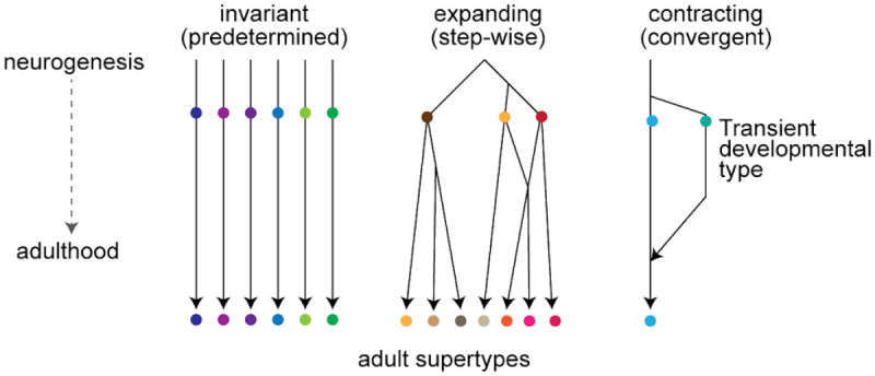
MCs follow an invariant (predetermined) while nMCs follow a expanding (step-wise) mode of diversification. These two modes were described and modified from Shekhar et al., 2022³³. A third mode of contracting (convergent) mode of diversification is exemplified by LRPs.

For MCs, developmental diversification appears to be largely predetermined—likely established embryonically and maintained postnatally—such that early developmental clusters map directly onto adult supertypes. Many MC subtypes emerge early and remain stable, reinforcing the idea of a developmentally pre-specified trajectory. Conversely, nMCs exhibited a more gradual, stepwise diversification, with many developmental clusters mapping to multiple adult supertypes, reflecting postmitotic plasticity. Consistent with a recent preprint by the Allen Institute, Gao et al.⁵⁴, we found that some SST+ supertypes (e.g., 226, 227, 229) only emerge later in development. Moreover, only 3 out of 19 SST+ supertypes (0215, 0219, and 0228) stably maintain their relative abundance from P1 to adulthood, highlighting the dynamic nature of SST+ interneuron maturation.

An intriguing implication of our findings is that nMC neurons retain the capacity to alter their identity post mitotically. Supporting this idea of fluid model of cell fate acquisition, a recent preprint by Alex Pollen’s laboratory reports that a fraction of mouse SST+ interneurons, when transplanted in human organoids, begin to express Pvalb⁷⁶. Considering that some of the developing nMCs map to adult Pvalb+ cells, we speculate that these post-mitotic populations are intrinsically amenable to identity..

A convergent model of diversification in LRP neurons

One striking observation in our study is the unique ‘contracting’ mode of diversification observed in LRPs (Fig. 8). LRP1 and LRP2.1 are transcriptionally distinct clusters that diverge into separate developmental trajectories as early as P5. Our re-analysis of datasets⁶⁸ from Bax cKO mice demonstrates that LRP2.1 is selectively lost from P7 onwards due to programmed cell death.

Programmed cell death is a general developmental hallmark of cortical inhibitory neurons^62–67. This form of cell pruning was thought until now to target inhibitory neurons indiscriminately. We show here that programmed cell death can also target specific inhibitory populations with exquisite precision, providing a powerful mechanism for fine sculpting of cortical circuits.

Moreover, this mechanism appears to be conserved in humans. In the developing human cortex, LRP2.1 peaks at GW18–20 and is eliminated by birth, coinciding with the completion of programmed cell death in the central nervous system⁷². The parallel trends in mice and humans suggest that selective pruning of LRP2.1 is an evolutionarily conserved strategy to fine tune the repertoire of inhibitory neurons. Collectively, our findings challenge the conventional view that inhibitory neurons follow a unidirectional and unimodal diversification trajectory by demonstrating the existence of a transient population, LRP2.1, that is selectively eliminated during postnatal cortical development.

Possible implications of transient LRP2.1 neurons

The transient nature of LRP2.1 raises questions about its function during early cortical development. Transient neuronal populations, such as subplate neurons⁷⁷, Cajal-Retzius cells^78,79, and early (first wave) oligodendrocytes⁸⁰, are known to influence brain development by shaping circuits and connectivity.^78,81–86.^6,87. Prior studies indicate that from P4 to P6, SST+ neurons in L5b receive short-lived excitatory inputs from thalamic projections, which disappear by P7^6,87. Given the transient nature of LRP2.1, it is possible these cells serve as a transient post-synaptic partner for thalamic projections in L5b. The programmed elimination of LRP2.1 by P7, and the consequent loss of these transient synaptic connections, coincides with the emergence of stable thalamic projections to L4. Future studies examining the axonal projections and synaptic partners of LRP2.1 could provide deeper insights into the function of this transient neuronal population.

In conclusion, our study presents a modular scRNAseq computational pipeline for enriching and integrating rare neuronal populations, leading to the construction of the most comprehensive developmental atlas of SST+ cortical interneurons to date. We reveal three distinct modes of neuronal diversification—invariant, expanding, and contracting. Notably, we describe a unique contracting trajectory in long-range projecting neurons, where early diversity is downscaled through selective programmed cell death. Additionally, we identified a transient cell type, termed the LIM (Long-range, Inhibitory, Minority population) neuron, which is evolutionarily conserved. These findings provide a data-rich foundational basis for understanding how neuronal diversity is generated and refined during the development of the mammalian cortex

Methods

Mouse models

The mouse lines used in this study are: WT C57BL/6J (Strain #:000664, RRID:IMSR_JAX:000664), Sst^Cre [B6N.Cg-Sst^{tm2.1(cre)Zjh/J}] (Strain#:018973, IMSR_JAX:018973)⁵⁰, RCE [(B6.Gt(ROSA)26Sort^{m1.1(CAGEGFP)Fsh}] (Strain#: 032037, RRID:MMRRC_032037-JAX)⁸⁸, RC:FLTG [B6.Cg Gt(ROSA)26Sort^{m1.3(CAG-tdTomato,-EGFP)Pjen/J}] (Strain#:026932, RRID:IMSR_JAX:026932)⁸⁹ and Nkx2.1^flp [Nkx2-1^{tm2.1(flpo)Zjh/J}] (Strain#:028577, RRID:IMSR_JAX:028577)⁹⁰. All adult mice were housed in groups and kept on a reverse light/dark cycle (12/12 h) regardless of genotype. Only time-mated pregnant female mice were housed individually. Male and female mice were used in all experiments. SST+ cells labelled by Sst^Cre mice were crossed with RCE reporter mice containing a floxed-stop cassette upstream of enhanced green fluorescent protein (EGFP) in the ROSA gene locus to obtain Sst^Cre;RCE^fl/+. In some experiments, we isolated MGE-derived cells, by using Nkx2.1^flp; RC:FLTG. All mice were maintained on a C57Bl/6 background and housed under a 12 h light/dark cycle with ad libitum access to food and water. All procedures were approved by KU Leuven and Scripps animal welfare committees.

Tissue preparation for FACS

Tissue preparation was similar to Fisher et al., (2024)²³. These include samples from DS19, DS20, DS21, DS22, DS23 and DS24. Briefly, all solutions used in this procedure have an osmolarity of 290 ± 20 mOsm/kg. For E16.5 and P1, tissue from 3 animals was pooled together. For P5, tissue from 1 and 2 animals was pooled together. The neocortex of E16.5, P1 and P5 SST^cre/+;RCE mice were dissected in an ice-cold HBSS buffer supplement with 25 mM of glucose. Tissue was cut into small pieces and digested for 10 min at 34°C with carbogen oxygenation using 30ml of dissociation buffer solution, pH7.5, with the following composition: 0.2 mg/ml pronaseE (Sigma), 50 mM of trehalose, 10 mM glucose, 0.8 mM kynurenic acid, 0.05 mM APV, 0.09 M Na₂SO₄, 0.03 M K₂SO₄ and 0.014 M MgCl₂. After 10 mins of incubation, E16.5 tissue was incubated at 34° for 5 more minutes with 375 μl of 10mg/ml DNAse while P1 and P5 tissue was incubated for 5 more minutes with 375 μl of 10mg/ml DNAse and 750μl of 10mg/ml liberase (Sigma). Post enzymatic digestion, tissues were washed once in an ice-cold dissociation buffer without enzyme. Tissue was mechanically triturated into single cells in 0.5 ml (for E16.5) or 5ml (for P1 and P5) of OptiMEM (Invitrogen) supplement with 2% Trehalose, 10 mM glucose, 0.8 mM kynurenic acid and 0.05 mM APV using a volumetric pipette. For P1 and P5 tissue, myelin was removed by overlaying single cell suspension on top of a 20% percoll and centrifuge at 700 g for 10 mins at 4 °C. The cell pellet was resuspended in 400 ul of OptiMEM with 2% Trehalose, 10 mM glucose, 0.8 mM kynurenic acid and 0.05 mM APV and tissue chunks were eliminated by passing cells suspension through a 40 mm cell strainer (BD).

For sample DS18 only, pregnant C56BL/6 dams carrying E18.5 embryos, previously injected intraventricularly with AAV expressing eYFP, were anesthetized with isoflurane and sacrificed by decapitation. The uterus was removed, the embryos were moved into cold Leibovitz’s L15 medium supplemented with 7 mM HEPES, and each embryo was decapitated. From each brain a section of the neocortex, corresponding roughly to S1, was dissected out with a micro-knife, avoiding the underlying striatal tissue. Tissue from 4–5 embryos of the same litter was pooled. Tissue sections were dissociated into single cell suspensions using the Worthington Tissue Dissociation Kit; the papain, DNAse, and albumin ovomucoid inhibitor solutions were reconstituted and oxygenated according to the manufacturer’s instructions. Tissue was digested in papain/DNAse for 15 min at 37° with carbogen oxygenation, triturated in EBSS using 1 mL lo-bind pipette tips, and then the cell suspension was mixed with albumin ovomucoid inhibitor/DNAse and centrifuged at 230g for 5min in a swinging bucket centrifuge. Cells were resuspended in an OptiMEM-trehalose media (OptiMEM supplemented with 50 mM of trehalose, 10 mMglucose, 0.5 mM kynurenic acid, 0.025 mM APV, 4 mM MgCl₂, 0.2 mM HEPES). Debris was removed by overlaying the suspension on top of a 5% Optiprep gradient and centrifuging at 100g for 10 mins. The cell pellet was resuspended in 500 uL of optimem-trehalose media, and DAPI and DRAQ5 were added to a final concentration of 1uM.

For dataset DS23, after myelin removal the cell pellet was resuspended in 1ml of 3% Glyoxal with the following composition: 2.8 ml Nuclease Free H₂0, 0.79 ml 100%EtOH, 0.31ml 40% Glyoxal (Sigma 50649), 30ul acetic acid, ph 4–5, for 15 min at 4° shaking. After incubation, cells were centrifuged at 800g for 10m at 4° and resuspended in 500ul of 1X PBS supplemented with 1% BSA and tissue chunks were eliminated by passing cells suspension through a 40 mm cell strainer (BD).

Cell isolation and 10X Genomics scRNAseq

GFP+ and DAPI negative for live samples and GFP+ and Fixable Viability Dye eFluor 780 negative cells for fixed samples were isolated using fluorescence-activated cell sorting (FACS) with a flow cytometer (BD Aria Fusion) using a 100 μm nozzle, about 3000–5000 events per second, at purity mode, and collected directly in 600 μl (cold 4 deg) of OptiMEM with 2% Trehalose, 10 mM glucose, 0.8 mM kynurenic acid and 0.05 mM APV solution in a 1.5-ml LoBind (Eppendorf) tubes precoated with 3% BSA overnight. We limited the FACS procedure to a maximum sort time of 25 mins to ensure high cell survival. We collected 20,000 to 30,000 cells for each sample. We centrifuge the collect cells at 600g for 5 minutes at 4° and resuspend the FACS cells in 40 μl of OptiMEM with 2% Trehalose, 10 mM glucose, 0.8 mM kynurenic acid and 0.05 mM APV. To determine cell number and viability, 5 μl of Trypan Blue was added to 5 μl of cells and cells were counted on a hemocytometer. In all experiments, we only proceed toward scRNA-seq with > 80% viability. About 12000 isolated single cells for each sample were loaded onto a custom droplet encapsulation platform, Hy Drop⁹¹, for single-cell capture. cDNA library preparation was performed following the 10X Genomic commercial kit CG000315. RNA-seq was performed using BGI MGISEQ-2000 and Illumina NovaSeq 6000 v1.5.

For sample DS18, cell suspension was sorted for live eYFP+ cells using an Astrios EQ sorting flow cytometer with a 100 um nozzle at 2-way purity. Sorted cells were collected in 0.5 ml of cold FACS media (OptiMEM supplemented with 50mM of trehalose, 10mMglucose, 0.5 mM kynurenic acid, 0.025 mM APV, 0.2 mM HEPES). Approximately 20,000 cells were collected. Cells were centrifuged at 200g for 15 minutes at 4° in a swinging bucket centrifuge and resuspended them in about 20 μL of FACS media. 5 μL of the cell suspension was taken out for cell counting and viability with a Countess, and we only used suspensions with >80% live cells. About 9000 isolated single cells for each sample were loaded onto a 10X Genomic single-cell chip for GEM formation and cDNA library preparation. RNA-seq was performed using an Illumina Nextseq200 P2 flow cell.

Shallow and deep scRNAseq

cDNA libraries were sequenced at two different depths. For shallow sequencing, we targeted a sequencing depth of 5,000 reads per cell; the actual achieved read number was 8,227.5 +/− 793.5 (mean +/− s.d.). For deep sequencing, we targeted 50,000 reads per cell; the actual read number achieved was 61,384 +/− 20,484.

Data pre-processing

Sequencing data were prepared for analysis by application of the 10X CellRanger pipeline. First, Illumina and BGI BCL output files were de-multiplexed into FASTQ format files. Features counts were computed for individual GEM wells. STAR aligner⁹² was applied to perform splicing aware alignment to the mm10 reference genome, and then reads were bucketed into exonic, intronic, and intergenic categories. Reads were classified as confidently aligned if they corresponded to a single gene annotation. Only confidently aligned reads were carried forward to UMI counting. A cell calling algorithm in conjunction with the barcode rank plot was applied to filter low RNA content cells and remove empty droplets. The output is a read count matrix. For publicly available datasets we downloaded raw count matrices. We used the R package Seurat (v 4.3.0.1) to perform the bulk of our subsequent data analysis, including filtering, normalization, scaling, and other downstream processing.

Sample processing and filtering of Sst+ cells (Module 1)

Each sample has been first processed separately for cell filtering and identification of cortical Sst+ neurons. We discarded any genes detected in fewer than 10 cells before filtering low quality cells. Cells were retained if they met the following criteria: (i) unique gene count > 700, (ii) mitochondrial gene content < 10%, (iii) ln(total UMI) > mean(ln(total UMI))-2sd(ln(total UMI)). To assess cell cycle phase differences in our dataset, we utilized the CellCycleScoring function from Seurat. Cell cycle phase scores were calculated for each cell using predefined gene lists for the S phase and G2M phase. Normalization and scaling of reads were performed using the R package Seurat, with the functions NormalizeData() and ScaleData(). During scaling, the number of total genes, percentage of mitochondrial gene expression and cell cycle phase difference score were regressed out to remove unwanted sources of variation from the data. Highly variable genes were defined using the Seurat function FindVariableFeatures() and Principal Component Analysis (PCA) was performed with the function RunPCA(). Doublets were identified using the scDblFinder⁹³ (v 1.12.0) algorithm with doublet rate set to 0.07. Cell clustering annotations were provided to scDblFinder, derived by applying TransferData() function to the cluster labels of our previously published dataset²³ using anchors identified by FindTransferAnchors() function on top 40 principal components. The optimal number of principal components was estimated performing a cross-validation on Principal Component Analysis (PCA)⁹⁴ and the resulting number of components was used as input to compute a k-Nearest Neighbors (k-NN) graph further refined into a Shared Nearest Neighbor (SNN) by the Seurat function FindNeighbors(). Clusters were defined using the Louvain algorithm implemented in FindClusters() function. Uniform manifold approximation and projection (UMAP) embedding was also computed running RunUMAP() with the estimated optimal principal components. We selected cells belonging to clusters expressing Sst gene, discarding “stressed” clusters, characterized by high expression of heat shock genes and lower average UMI, and clusters expressing Meis2, QC metric similar to Fisher et al., 2024²³.

Integrability testing of datasets (Module 2)

To test if any given dataset can be used to generate an integrative atlas, we selected only datasets containing at least 1,000 high-quality Sst+ cells, as identified using previously described methods. The integrability of each dataset with our reference atlas (Atlas-v0) was evaluated using three criteria: Anchor points, Neighborhood composition, and kBET⁵² rejection test.

1. Anchor Points - The integration anchors between the testing datasets and Atlas-v0 were identified using the FindIntegrationAnchors() function in the Seurat package, with reduction = ‘cca’. The mean number of anchors for each testing dataset relative to Atlas-v0 was computed, and a mean anchor count greater than 2,000 was set as the acceptance criterion.

2. Neighborhood composition - The testing dataset was integrated with Atlas-v0 using the IntegrateData() function based on the previously identified anchors to create a corrected gene expression matrix. This matrix was scaled using the ScaleData() function, and principal components were estimated using the RunPCA() function. Pairwise Euclidean distances were computed between the test dataset cells and the nearest reference atlas (Atlas-v0) cells in the integrated PCA space. The minimum distance for each test dataset cell was extracted and added as a metadata feature. The percentage of test dataset cells with nearest neighbors comprising at least half the expected fraction of reference atlas cells was calculated for increasing k-values (ranging from 5 to 200, in increments of 5).

   k-NN Computation: Nearest neighbors were identified using the dbscan::kNN() function in PCA space. For each k-value, the proportion of cells meeting the threshold of reference atlas cell representation was computed. A cell percentage exceeding 50% for k = 75 was used as the acceptance criterion.

3. kBET Rejection Rate - The kBET⁵² rejection rate (version 0.99.6) was calculated to evaluate how well the testing dataset and reference atlas (Atlas-v0) were integrated in the corrected PCA space. A rejection rate below 50% was set as the acceptance criterion.

Only datasets meeting all three criteria (anchor points, neighborhood composition, and kBET rejection rate) were included in the generation of Atlas-v1.

Data Integration and annotation (Module 3)

Individual samples were integrated into a single object using canonical correlation analysis (CCA)⁹⁵. Anchors were identified across samples with FindIntegrationAnchors() function with parameters reduction= ‘cca’, k.filter=100, k.score=15 and anchor.features=2000. A batch corrected gene expression matrix was then computed using IntegrateData() function. The resulting matrix was scaled using ScaleData() function, regressing for number of total genes, percentage of mitochondrial gene expression and cell cycle score. PCA was performed with RunPCA() function, and the optimal number of principal components was determined via cross-validation. Clustering was computed with FindNeighbors() and FindClusters() functions, based on the optimal number of principal components estimated. Uniform manifold approximation and projection (UMAP) embedding was computed using RunUMAP() function. Cells within “stressed” clusters characterized by high expression of heat shock genes and low average UMI, doublets, or clusters showing high expression of mitochondrial genes were further removed. Resulting cells were annotated to major groups of cortical Sst+ neurons (LRP, MC, and nMC) using annotated cells from the base atlas. This annotation was achieved by applying the TransferData() function on anchors identified between each sample and the base atlas using the FindTransferAnchors() function. Each cell was annotated to the group that achieved the maximum score.

Iterative Clustering of Atlas-v1

Clustering algorithm was performed separately on each major group of cortical Sst+ neurons (LRP, MC and nMC). To compute clusters, we followed an iterative approach characterized by the following steps:

1. Sample filtering. Remove samples with less than 20 cells.

2. Data integration and clustering. Perform data integration using canonical correlation analysis and apply clustering as previously described. Clustering was computed at resolutions of 0.1, 0.2, 0.3, 0.4 and 0.5 using a kNN graph built with k=20 using the optimal number of principal components (PCs). Duplicated clustering (clusters from different resolutions that result in the same cell annotation) were considered only once.

3. Clustering stability evaluation. We performed 20 data sub-samplings, each time sampling 80% of the cells without replacement, and repeated the clustering procedure for all selected resolutions on each subsample. Jaccard indices were calculated for each cluster at each resolution by comparing the original clusters with those obtained from each subsample. We defined a stable cluster as one with Jaccard index⁹⁶ greater than 0.75 in at least 75% of the subsamples. A stable set of clusters was defined as one where more than 70% of the cells belonged to stable clusters and stable clusters accounted for more than 60% of the total clusters. If no clustering was found to be stable, the iteration was stopped, and the cluster label obtained in the previous iteration was assigned as the final identity of all the cells. Otherwise, among stable clustering, we selected the resolution that produced the higher percentage of cells within stable clusters. If two or more clustering resulted in the same percentage, the resolution with the higher number of clusters was chosen.

4. Cluster identity evaluation and merging. All clusters with fewer than 150 cells were merged with their closest cluster: centroids were calculated in batch corrected PCA space and the closest cluster was defined as the one with the smallest Euclidean distance between centroids. For each resulting cluster, marker genes were identified by comparing gene expression with all other cells not belonging to the cluster. FindMarkers() function from Seurat was used with parameters logfc.threshold=1 and only.pos = TRUE. Genes with an adjusted p.value lower than 0.01 were selected and the sum of the min (-log₁₀(p.val_adj), 20) values across all selected genes was calculated. If the resulting value was less or equal to 60, the cluster was merged with its closest cluster as previously described.

5. Process iteration. After identity evaluation, if only one cluster remained, the iteration was stopped and the cluster label obtained in the previous iteration was assigned as the final identity of the cluster. If more than one cluster remained, the process was repeated from step 1 to step 5 for all clusters with 300 cells or more. Clusters with fewer than 300 cells were returned as the final identity.

6. After all clustering iterations ended, cells removed at step 1 of each iteration were annotated. The k-NN constructed during iteration 1 was used to identify the nearest neighbours for each removed cell, and each cell was assigned to the cluster most represented among its nearest neighbours.

Cell annotation validation

To validate cell identities, we performed five-fold cross-validation, taking 20% of the data as a test set and the remaining 80% as the training set. We computed differentially expressed genes for all clusters in the five training sets using FindMarkers() function with options logfc.threshold=ln(1.5), only.pos=TRUE, min.pct=0.5. We then proceed in a pairwise fashion, using randomForest⁹⁷ R package (v 4.7–1.1) we trained a random forest classifier with 100 trees on each pair of clusters in the training data using only the top 10 differentially expressed genes, ranked by logFC, from each cluster. This classifier was used to predict the identity of cells in the test set. Following five-fold cross-validation, we have a predicted identity for every cell for each pairwise comparison of clusters. The above procedure was repeated for a total of 10 iterations. From the consistency of the outcome across these iterations, we extracted a measure of the stability of the cell classification.

Cell annotation to adult counterparts

To annotate our data to their adult counterparts, we used the MapMyCells¹⁵ algorithm, using the 10x Whole Mouse Brain (CCN20230722) as reference taxonomy and using the hierarchical mapping as chosen algorithm. Briefly, to annotate unlabelled cells to their corresponding class, subclass, supertype, or cluster, the algorithm compares the gene expression of each unlabelled cell with the average expression profile of each child node at every level of the hierarchy. This comparison is performed using marker genes that effectively discriminate among child nodes, assigning a vote to the child node with the highest Pearson correlation. For robustness, the process is repeated 100 times, randomly selecting 90% of all marker genes every time. A cell is assigned to the child node with the highest number of votes, and cell labels were considered valid if 90 out of 100 annotations assigned the cell to the same child node. We then defined a 1:1 matching between one of our clusters and an annotated supertype if at least 65% of the cells within the cluster were assigned to that supertype, and if the majority of all cells annotated to that supertype originated from that cluster, representing at least 30% of all cells annotated to the supertype.

Trajectory and Pseudotime analysis

We performed trajectory analysis on the LRP clusters. First, we computed gene modules that captured distinct sources of variation within the data. We used the R package Antler⁵⁶ (v0.9.0) to generate these modules. Computation began with a normalized counts-per-million matrix. Genes present in fewer than 10 cells were discounted from the computation. Genes were filtered prior to clustering to retain only those genes having Spearman correlation with at least 5 other genes at value 0.3. These genes were clustered hierarchically using Spearman correlation as a dissimilarity metric. This hierarchical clustering was repeated over many iterations, with a heuristic algorithm determining an optimal number of modules. At each iteration, modules were discarded if they failed to meet validity thresholds on the expression level of individual genes. At the terminal iteration, all modules met the validation criteria and were returned as the final set of gene modules. To understand the module contents, we performed functional enrichment on each module and examined gene ontology terms. We selected 335 genes from modules associated with terms including “neuron differentiation”, “axon development”, and “synapse assembly”. We computed Diffusion Maps with Destiny⁹⁸ R package (v 3.12.0) on the corrected expression matrix, considering only the selected genes. The eigenvalues of the diffusion map transition matrix were used as diffusion components for low-dimensional embedding. The pseudotime for each cell was computed from the full transition matrix using the DPT() function and represents a notion of diffusion distance from a root cell. The root cell was identified as the cell from the earliest age samples that had the highest number of early sample cells in its neighborhood (computed on diffusion components). From this analysis, we inferred linear branches diverging from an initial shared state. We then identified genes exhibiting continuous changes over pseudotime, by fitting each gene’s expression vector to pseudotime using a generalized additive model (GAM), with the gam() function from mgcv⁹⁹ R package (1.9–0). Genes were classified as early genes (negatively correlated with pseudotime) or late genes (positively correlated with pseudotime). Late genes were further subdivided into those specifically expressed in only one branch.

Saturation analysis

We subsampled cells without replacement at percentages ranging from 5% to 95% in 5% intervals. For each percentage, we generated 10 different subsamples. To estimate the saturation point, we calculated several metrics. First, we computed robust Hausdorff Distance between each subsample and the original dataset in the batch corrected PCA space, selecting the 50th largest value as the distance measure. Next, we identified marker genes for each cluster in each subsample and recorded the total number of marker genes. Additionally, we calculated the absolute differences in mean expression for marker genes between the subsamples and the entire atlas for each cluster. The mean of differences across clusters were summed over all differentially expressed genes. Finally, we assessed the fraction of clusters that maintained their identity in each subsample. For this, cluster centroids were calculated based on gene expression vectors, and clusters from the whole dataset were matched to the centroids of the subsamples using MetaNeighborUS() function from MetaNeighbor⁵⁵ R package (v 1.18.0). Clusters with an AUROC score greater than 0.9 when matched to their centroids in the subsample were considered to have retained their identity. For each subsampling percentage, we computed the mean scores for all metrics (robust Hausdorff Distance, number of differentially expressed genes, sum of absolute differences in mean expression, and percentage of clusters preserving their identity) across the 10 subsamples. The inflection point, indicating the saturation percentage, was identified as the point where the second derivative of the metrics changed sign.

Cloning of viral vector and generation AAV

The AAV enhancer plasmid, pAAV-eHGT-m600-sYFP2⁶⁰, was provided by Boaz Levi (Allen Institute). To generate pAAV-eHGT-m600-dio-sYFP2, sYFP2 was removed with restriction enzymes BamH1 and EcoRV, and the backbone was isolated by gel purification. The insert, dio-sYFP2, with a 20-bp homology on both 5’- and 3’-end to the backbone was synthesized by Twist Bioscience as a gene fragment. Backbone and insert were assembled by NEBuilder Hi-Fi DNA Assembly (NEB, E2621L) per manufacturer recommendation and transformed into NEB Stable competent cells (NEB, C3040I). Using the transfer vectors pAAV-eHGT-600m-sYFP2 and pAAV-eHGT-600m-dio-sYFP2, AAV2/9 were custom generated by BrainVTA at a viral titre of >3 × 10¹³ vg/ml.

Neonatal injection of AAV

AAV injections were performed on P0 wild-type CD1 mice or SST^Cre/+ mice under hypothermia-induced anesthesia. Injections into the lateral ventricle were conducted using glass micropipettes (1B120F-4, World Precision Instruments) connected to a pressure microinjector device (μPUMP, World Precision Instruments). The injection site was identified at half the distance from the lambda suture to each eye. The glass micropipette was inserted perpendicularly into the skull to a depth of approximately 2 mm, with slight resistance decrease indicating entry into the lateral ventricle. Approximately 1 μL of the virus (AAV2/9-eHGT-600m-SYFP2 or AAV2/9-eHGT-600m-dio-SYFP2) was rapidly injected into each ventricle. Following the injections, pups were placed on a warming pad to recover until they could move normally and were then returned to their mother.

Histology and immunochemistry

Adult and postnatal pups were deeply anaesthetized with an intraperitoneal injection of ketamine (87 mg per kg body weight) and xylazine (13 mg per kg body weight) and transcardially perfused with ice-cold phosphate-buffered saline (PBS) followed by 4% paraformaldehyde (PFA). The brains were isolated and incubated overnight in 4% PFA on a slow-speed rocking platform at 4 °C. Tissue was washed with PBS, incubated in 10% followed by 30% sucrose in PBS and cut on a freezing microtome into 100 μm coronal sections, and stored in cryoprotectant solution (30% glycerol, 30% ethylene glycol in PBS) at −20 °C or processed or free-floating immunohistochemistry. Coronal sections were stained using the following primary antibodies: rabbit anti-Dach1 (1:500, Proteintech, 10914–1-AP), chicken anti-GFP (1:3000, Aves Lab, GFP-1020), rabbit anti- MafB (1:500, Sigma Aldrich, HPA005653), and rabbit anti- Nitric Oxide Synthase 1 - NOS1 (1:1000, Immunostar, 24287). Tissue was blocked with 2% BSA, 10% goat serum in 0.25% triton-X-100-PBS for 1h at RT. Primary antibodies were incubated overnight at 4 °C in 2% BSA, 10% goat serum in 0.25% triton-X-100-PBS. The following secondary antibodies conjugated to Alex Fluor dyes were used: goat anti-chicken IgY (H+L) Alexaplus 488 (Thermofisher A32931), and donkey anti-rabbit IgG (H+L) Alexaplus 647 (Thermofisher A32795). Secondary antibodies were all used at 1:1000, incubated for 2 h at RT, followed by 4’,6-diamidino-2-fenylindool (DAPI) (5 μM, Sigma, D9542) for 10 minutes at RT. Sections were washed three times for 10 minutes with 0.1% triton-X in PBS after secondary and DAPI staining. Brain sections were mounted in Mowiol-DABCO (25% Mowiol, Sigma, 81381, 2,5% DABCO, Sigma, D27802). Brain sections were imaged using an inverted Ti2-E Nikon microscope with a Crest Optic X-light V3 spinning disk. Subsequent image processing was performed using FIJI or Matlab.

Image Analysis and Quantification of LRP1 and LRP2.1 by histology

Two types of staining were used for the analysis: (i) GFP and Dach1, and (ii) GFP and MafB. LRP1 was defined as GFP+ cells expressing high levels of MafB but low levels of Dach1. In contrast, LRP2.1 was defined as GFP+ cells expressing low levels of MafB but high levels of Dach1. Quantification of Dach1 and MafB expression levels was performed using MATLAB with a customized script, which is publicly available on GitHub. Briefly, GFP+ cells were selected based on a manual thresholding function determined by the user. For each GFP+ cell, the centroid was identified and expanded into a circular region with a 4-pixel radius. The mean intensity signal of either MafB or Dach1 within this circular region was then calculated. For Dach1, mean intensity values in the GFP+ cells that were at least 2× above the background intensity were classified as high Dach1. For MafB, since all GFP+ cells expressed MafB, the intensity values in GFP+ cells were fitted to a normal distribution. Cells with MafB intensity levels above the 75th percentile (mean + 0.524 standard deviations) were classified as high MafB.

Data availability

All previously published scRNAseq data are downloaded and available on GEO per table 1. Upon publication, these data will be freely accessible. For the review process, the raw data can be accessed by GEO. DS18 - serie GSE280655, access token: gzgrwmgmvfarvin. DS19 – 22 GSE271016 access token: ctwvmwsklretpwz. DS23, 24, GSE271947, access token: ylcpcmucdtslnch. Dev-SST-v1 can be accessed through a web interface https://shiny.gbiomed.kuleuven.be/AtlasLL/ or the final seurat object can be requested by contacting Lynette Lim (lynette.lim@kulevuen.vib.be). All customised analysis codes written in R and Matlab used to generate Dev-SST-atlas and individual figure plots/ panels can be found on GitHub: https://github.com/Limlab-VIBCBD/Dev-SST-atlas.

References

- 1.Wonders C. P. & Anderson S. A. The origin and specification of cortical interneurons. Nat. Rev. Neurosci. 7, 687–696 (2006). [DOI] [PubMed] [Google Scholar]
- 2.Kessaris N. & Denaxa M. Cortical interneuron specification and diversification in the era of big data. Curr. Opin. Neurobiol. 80, 102703 (2023). [DOI] [PubMed] [Google Scholar]
- 3.Ichim A. M. et al. The gamma rhythm as a guardian of brain health. eLife 13, e100238 (2024). [DOI] [PMC free article] [PubMed] [Google Scholar]
- 4.Fishell G. & Kepecs A. Interneuron Types as Attractors and Controllers. Annual Review of Neuroscience 43, 1–30 (2020). [DOI] [PMC free article] [PubMed] [Google Scholar]
- 5.Schuman B., Dellal S., Pröonneke A., Machold R. & Rudy B. Neocortical Layer 1: An Elegant Solution to Top-Down and Bottom-Up Integration. Annual Review of Neuroscience 44, 221–252 (2021). [DOI] [PMC free article] [PubMed] [Google Scholar]
- 6.Tuncdemir S. N. et al. Early Somatostatin Interneuron Connectivity Mediates the Maturation of Deep Layer Cortical Circuits. Neuron 89, 521–535 (2016). [DOI] [PMC free article] [PubMed] [Google Scholar]
- 7.Lim L., Mi D., Llorca A. & Marín O. Development and Functional Diversification of Cortical Interneurons. Neuron 100, 294–313 (2018). [DOI] [PMC free article] [PubMed] [Google Scholar]
- 8.Hanson K. L., Greiner D. M. Z., Schumann C. M. & Semendeferi K. Inhibitory Systems in Brain Evolution: Pathways of Vulnerability in Neurodevelopmental Disorders. Brain, Behav. Evol. 1–20 (2024) doi: 10.1159/000540865. [DOI] [PMC free article] [PubMed] [Google Scholar]
- 9.Marin O. Cellular and molecular mechanisms controlling the migration of neocortical interneurons. Eur. J. Neurosci. 38, 2019–2029 (2013). [DOI] [PubMed] [Google Scholar]
- 10.Marin O. Developmental timing and critical windows for the treatment of psychiatric disorders. Nature Medicine 22, 1229–1238 (2016). [DOI] [PubMed] [Google Scholar]
- 11.Marin O. Interneuron dysfunction in psychiatric disorders. Nat. Rev. Neurosci. 13, 107–120 (2012). [DOI] [PubMed] [Google Scholar]
- 12.Ward C., Sjulson L. & Batista-Brito R. The function of Mef2c toward the development of excitatory and inhibitory cortical neurons. Front. Cell. Neurosci. 18, 1465821 (2024). [DOI] [PMC free article] [PubMed] [Google Scholar]
- 13.Ferranti A. S., Luessen D. J. & Niswender C. M. Novel pharmacological targets for GABAergic dysfunction in ADHD. Neuropharmacology 249, 109897 (2024). [DOI] [PMC free article] [PubMed] [Google Scholar]
- 14.Lodato S. & Arlotta P. Generating Neuronal Diversity in the Mammalian Cerebral Cortex. Annual Review of Cell and Developmental Biology 31, 699–720 (2015). [DOI] [PMC free article] [PubMed] [Google Scholar]
- 15.Yao Z. et al. A high-resolution transcriptomic and spatial atlas of cell types in the whole mouse brain. Nature 624, 317–332 (2023). [DOI] [PMC free article] [PubMed] [Google Scholar]
- 16.(BICCN), B. I. C. C. N. et al. A multimodal cell census and atlas of the mammalian primary motor cortex. Nature 598, 86–102 (2021). [DOI] [PMC free article] [PubMed] [Google Scholar]
- 17.Yao Z. et al. A taxonomy of transcriptomic cell types across the isocortex and hippocampal formation. Cell 184, 3222–3241.e26 (2021). [DOI] [PMC free article] [PubMed] [Google Scholar]
- 18.Chartrand T. et al. Morphoelectric and transcriptomic divergence of the layer 1 interneuron repertoire in human versus mouse neocortex. Science 382, eadf0805 (2023). [DOI] [PMC free article] [PubMed] [Google Scholar]
- 19.Gouwens N. W. et al. Integrated Morphoelectric and Transcriptomic Classification of Cortical GABAergic Cells. Cell 183, 935–953.e19 (2020). [DOI] [PMC free article] [PubMed] [Google Scholar]
- 20.Zhang M. et al. Molecularly defined and spatially resolved cell atlas of the whole mouse brain. Nature 624, 343–354 (2023). [DOI] [PMC free article] [PubMed] [Google Scholar]
- 21.Dai R. et al. Precision and Accuracy of Single-Cell/Nuclei RNA Sequencing Data. bioRxiv 2024.04.12.589216 (2024) doi: 10.1101/2024.04.12.589216. [DOI] [Google Scholar]
- 22.Frazer S. et al. Transcriptomic and anatomic parcellation of 5-HT3AR expressing cortical interneuron subtypes revealed by single-cell RNA sequencing. Nature Communications 8, 14219 (2017). [DOI] [PMC free article] [PubMed] [Google Scholar]
- 23.Fisher J. et al. Cortical somatostatin long-range projection neurons and interneurons exhibit divergent developmental trajectories. Neuron 112, 558–573.e8 (2024). [DOI] [PubMed] [Google Scholar]
- 24.Mi D. et al. Early emergence of cortical interneuron diversity in the mouse embryo. Science (New York, N.Y.) 360, 81–85 (2018). [DOI] [PMC free article] [PubMed] [Google Scholar]
- 25.Shi Y. et al. Mouse and human share conserved transcriptional programs for interneuron development. Science 374, eabj6641 (2021). [DOI] [PubMed] [Google Scholar]
- 26.Mayer C. et al. Developmental diversification of cortical inhibitory interneurons. Nature 555, 457–462 (2018). [DOI] [PMC free article] [PubMed] [Google Scholar]
- 27.Lim L. et al. Optimization of interneuron function by direct coupling of cell migration and axonal targeting. Nature Neuroscience 21, 920–931 (2018). [DOI] [PMC free article] [PubMed] [Google Scholar]
- 28.Wu S. J. et al. Cortical somatostatin interneuron subtypes form cell-type-specific circuits. Neuron 111, 2675–2692.e9 (2023). [DOI] [PMC free article] [PubMed] [Google Scholar]
- 29.Nigro M. J., Hashikawa-Yamasaki Y. & Rudy B. Diversity and Connectivity of Layer 5 Somatostatin-Expressing Interneurons in the Mouse Barrel Cortex. The Journal of Neuroscience 38, 1622–1633 (2018). [DOI] [PMC free article] [PubMed] [Google Scholar]
- 30.Tremblay R., Lee S. & Rudy B. GABAergic interneurons in the neocortex: From cellular properties to circuits. Neuron 91, 260–292 (2016). [DOI] [PMC free article] [PubMed] [Google Scholar]
- 31.Telley L. et al. Temporal patterning of apical progenitors and their daughter neurons in the developing neocortex. Science 364, (2019). [DOI] [PubMed] [Google Scholar]
- 32.Taniguchi H., Lu J. & Huang Z. J. The Spatial and Temporal Origin of Chandelier Cells in Mouse Neocortex. Science 339, 70–74 (2013). [DOI] [PMC free article] [PubMed] [Google Scholar]
- 33.Shekhar K., Whitney I. E., Butrus S., Peng Y.-R. & Sanes J. R. Diversification of multipotential postmitotic mouse retinal ganglion cell precursors into discrete types. eLife 11, e73809 (2022). [DOI] [PMC free article] [PubMed] [Google Scholar]
- 34.Agmon A. & Barth A. L. A brief history of somatostatin interneuron taxonomy or: how many somatostatin subtypes are there, really? Front. Neural Circuits 18, 1436915 (2024). [DOI] [PMC free article] [PubMed] [Google Scholar]
- 35.Moreau M. X., Saillour Y., Cwetsch A. W., Pierani A. & Causeret F. Single-cell transcriptomics of the early developing mouse cerebral cortex disentangle the spatial and temporal components of neuronal fate acquisition. Dev. (Camb., Engl.) 148, (2020). [DOI] [PubMed] [Google Scholar]
- 36.Sambo D. et al. Cell type-specific changes in Wnt signaling and neuronal differentiation in the developing mouse cortex after prenatal alcohol exposure during neurogenesis. Front. Cell Dev. Biol. 10, 1011974 (2022). [DOI] [PMC free article] [PubMed] [Google Scholar]
- 37.Ruan X. et al. Progenitor cell diversity in the developing mouse neocortex. Proc. Natl. Acad. Sci. 118, e2018866118 (2021). [DOI] [PMC free article] [PubMed] [Google Scholar]
- 38.Garcia M. T. et al. Transcriptional profiling of sequentially generated septal neuron fates. eLife 10, e71545 (2021). [DOI] [PMC free article] [PubMed] [Google Scholar]
- 39.Loo L. et al. Single-cell transcriptomic analysis of mouse neocortical development. Nat. Commun. 10, 134 (2019). [DOI] [PMC free article] [PubMed] [Google Scholar]
- 40.Bella D. J. D. et al. Molecular logic of cellular diversification in the mouse cerebral cortex. Nature 595, 554–559 (2021). [DOI] [PMC free article] [PubMed] [Google Scholar]
- 41.Manno G. L. et al. Molecular architecture of the developing mouse brain. Nature 596, 92–96 (2021). [DOI] [PubMed] [Google Scholar]
- 42.Cheng S. et al. Vision-dependent specification of cell types and function in the developing cortex. Cell 185, 311–327.e24 (2022). [DOI] [PMC free article] [PubMed] [Google Scholar]
- 43.Nunnelly L. F. et al. St18 specifies globus pallidus projection neuron identity in MGE lineage. Nat. Commun. 13, 7735 (2022). [DOI] [PMC free article] [PubMed] [Google Scholar]
- 44.Kalish B. T. et al. Single-nucleus RNA sequencing of mouse auditory cortex reveals critical period triggers and brakes. Proc. Natl. Acad. Sci. 117, 11744–11752 (2020). [DOI] [PMC free article] [PubMed] [Google Scholar]
- 45.Allaway K. C. et al. Genetic and epigenetic coordination of cortical interneuron development. Nature 597, 693–697 (2021). [DOI] [PMC free article] [PubMed] [Google Scholar]
- 46.Wittmann M.-T. et al. scRNA sequencing uncovers a TCF4-dependent transcription factor network regulating commissure development in mouse. Dev. (Camb., Engl.) 148, (2020). [DOI] [PMC free article] [PubMed] [Google Scholar]
- 47.Bandler R. C. et al. Single-cell delineation of lineage and genetic identity in the mouse brain. Nature 601, 404–409 (2022). [DOI] [PMC free article] [PubMed] [Google Scholar]
- 48.Yuzwa S. A. et al. Developmental Emergence of Adult Neural Stem Cells as Revealed by Single-Cell Transcriptional Profiling. Cell Rep. 21, 3970–3986 (2017). [DOI] [PubMed] [Google Scholar]
- 49.Zheng G. X. Y. et al. Massively parallel digital transcriptional profiling of single cells. Nat. Commun. 8, 14049 (2017). [DOI] [PMC free article] [PubMed] [Google Scholar]
- 50.Taniguchi H. et al. A Resource of Cre Driver Lines for Genetic Targeting of GABAergic Neurons in Cerebral Cortex. Neuron 71, 995–1013 (2011). [DOI] [PMC free article] [PubMed] [Google Scholar]
- 51.Hu J. S., Vogt D., Sandberg M. & Rubenstein J. L. Cortical interneuron development: a tale of time and space. Development 144, 3867–3878 (2017). [DOI] [PMC free article] [PubMed] [Google Scholar]
- 52.Buttner M., Miao Z., Wolf F. A., Teichmann S. A. & Theis F. J. A test metric for assessing single-cell RNA-seq batch correction. Nat. Methods 16, 43–49 (2019). [DOI] [PubMed] [Google Scholar]
- 53.Marín O., Anderson S. A. & Rubenstein J. L. R. Origin and Molecular Specification of Striatal Interneurons. J. Neurosci. 20, 6063–6076 (2000). [DOI] [PMC free article] [PubMed] [Google Scholar]
- 54.Gao Y. et al. Continuous cell type diversification throughout the embryonic and postnatal mouse visual cortex development. bioRxiv 2024.10.02.616246 (2024) doi: 10.1101/2024.10.02.616246. [DOI] [Google Scholar]
- 55.Crow M., Paul A., Ballouz S., Huang Z. J. & Gillis J. Characterizing the replicability of cell types defined by single cell RNA-sequencing data using MetaNeighbor. Nature Communications 9, 884 (2018). [DOI] [PMC free article] [PubMed] [Google Scholar]
- 56.Delile J. et al. Single cell transcriptomics reveals spatial and temporal dynamics of gene expression in the developing mouse spinal cord. Development 146, dev173807 (2019). [DOI] [PMC free article] [PubMed] [Google Scholar]
- 57.Marin O. & Rubenstein J. L. R. A long, remarkable journey: Tangential migration in the telencephalon. Nat. Rev. Neurosci. 2, 780–790 (2001). [DOI] [PubMed] [Google Scholar]
- 58.Flames N. et al. Short- and Long-Range Attraction of Cortical GABAergic Interneurons by Neuregulin-1. Neuron 44, 251–261 (2004). [DOI] [PubMed] [Google Scholar]
- 59.Sánchez-Alcañiz J. A. et al. Cxcr7 Controls Neuronal Migration by Regulating Chemokine Responsiveness. Neuron 69, 77–90 (2011). [DOI] [PubMed] [Google Scholar]
- 60.Ben-Simon Y. et al. A suite of enhancer AAVs and transgenic mouse lines for genetic access to cortical cell types. bioRxiv 2024.06.10.597244 (2024) doi: 10.1101/2024.06.10.597244. [DOI] [Google Scholar]
- 61.Magno L., Oliveira M. G., Mucha M., Rubin A. N. & Kessaris N. Multiple embryonic origins of nitric oxide synthase-expressing GABAergic neurons of the neocortex. Front. Neural Circuits 6, 65 (2012). [DOI] [PMC free article] [PubMed] [Google Scholar]
- 62.Southwell D. G. et al. Intrinsically determined cell death of developing cortical interneurons. Nature 491, 109–113 (2012). [DOI] [PMC free article] [PubMed] [Google Scholar]
- 63.Priya R. et al. Activity Regulates Cell Death within Cortical Interneurons through a Calcineurin-Dependent Mechanism. Cell Rep. 22, 1695–1709 (2018). [DOI] [PMC free article] [PubMed] [Google Scholar]
- 64.Wong F. K. et al. Pyramidal cell regulation of interneuron survival sculpts cortical networks. Nature 557, 668–673 (2018). [DOI] [PMC free article] [PubMed] [Google Scholar]
- 65.Denaxa M. et al. Modulation of Apoptosis Controls Inhibitory Interneuron Number in the Cortex. Cell Rep. 22, 1710–1721 (2018). [DOI] [PMC free article] [PubMed] [Google Scholar]
- 66.Leon W. R. M. et al. The clustered gamma protocadherin PcdhγC4 isoform regulates cortical interneuron programmed cell death in the mouse cortex. Proc. Natl. Acad. Sci. 121, e2313596120 (2024). [DOI] [PMC free article] [PubMed] [Google Scholar]
- 67.Leon W. R. M. et al. Clustered gamma-protocadherins regulate cortical interneuron programmed cell death. eLife 9, e55374 (2020). [DOI] [PMC free article] [PubMed] [Google Scholar]
- 68.Wu S. J. et al. Pyramidal neurons proportionately alter the identity and survival of specific cortical interneuron subtypes. bioRxiv 2024.07.20.604399 (2024) doi: 10.1101/2024.07.20.604399. [DOI] [Google Scholar]
- 69.Bhaduri A. et al. An atlas of cortical arealization identifies dynamic molecular signatures. Nature 598, 200–204 (2021). [DOI] [PMC free article] [PubMed] [Google Scholar]
- 70.Velmeshev D. et al. Single-cell analysis of prenatal and postnatal human cortical development. Science 382, eadf0834 (2023). [DOI] [PMC free article] [PubMed] [Google Scholar]
- 71.Bershteyn M. et al. Human stem cell-derived GABAergic interneuron development reveals early emergence of subtype diversity followed by gradual electrochemical maturation. bioRxiv 2024.12.03.626662 (2024) doi: 10.1101/2024.12.03.626662. [DOI] [Google Scholar]
- 72.Zeiss C. J. Comparative Milestones in Rodent and Human Postnatal Central Nervous System Development. Toxicol. Pathol. 49, 1368–1373 (2021). [DOI] [PubMed] [Google Scholar]
- 73.Zhang Z. et al. Recovery of biological signals lost in single-cell batch integration with CellANOVA. Nat. Biotechnol. 1–17 (2024) doi: 10.1038/s41587-024-02463-1. [DOI] [PubMed] [Google Scholar]
- 74.Tyler S. R., Guccione E. & Schadt E. E. Erasure of Biologically Meaningful Signal by Unsupervised scRNAseq Batch-correction Methods. bioRxiv 2021.11.15.468733 (2023) doi: 10.1101/2021.11.15.468733. [DOI] [Google Scholar]
- 75.Monnier L. & Cournede P.-H. A novel batch-effect correction method for scRNA-seq data based on Adversarial Information Factorization. PLOS Comput. Biol. 20, e1011880 (2024). [DOI] [PMC free article] [PubMed] [Google Scholar]
- 76.Mostajo-Radji M. A. et al. Fate plasticity of interneuron specification. bioRxiv 2024.10.02.614266 (2024) doi: 10.1101/2024.10.02.614266. [DOI] [Google Scholar]
- 77.Marin-Padilla M. Early prenatal ontogenesis of the cerebral cortex (neocortex) of the cat (Felis domestica). A Golgi study. I. The primordial neocortical organization. Z. fur Anat. Entwicklungsgeschichte 134, 117–45 (1971). [DOI] [PubMed] [Google Scholar]
- 78.Soriano E. & Rio J. A. del. The Cells of Cajal-Retzius: Still a Mystery One Century After. Neuron 46, 389–394 (2005). [DOI] [PubMed] [Google Scholar]
- 79.Griveau A. et al. A Novel Role for Dbx1-Derived Cajal-Retzius Cells in Early Regionalization of the Cerebral Cortical Neuroepithelium. PLoSBiol. 8, e1000440 (2010). [DOI] [PMC free article] [PubMed] [Google Scholar]
- 80.Kessaris N. et al. Competing waves of oligodendrocytes in the forebrain and postnatal elimination of an embryonic lineage. Nat. Neurosci. 9, 173–179 (2006). [DOI] [PMC free article] [PubMed] [Google Scholar]
- 81.Gil-Sanz C. et al. Cajal-Retzius Cells Instruct Neuronal Migration by Coincidence Signaling between Secreted and Contact-Dependent Guidance Cues. Neuron 79, 461–477 (2013). [DOI] [PMC free article] [PubMed] [Google Scholar]
- 82.Supèr H., Soriano E. & Uylings H. B. M. The functions of the preplate in development and evolution of the neocortex and hippocampus. Brain Res. Rev. 27, 40–64 (1998). [DOI] [PubMed] [Google Scholar]
- 83.Sarnat H. B. & Flores-Sarnat L. Role of Cajal-Retzius and subplate neurons in cerebral cortical development. Semin. Pediatr. Neurol. 9, 302–308 (2002). [DOI] [PubMed] [Google Scholar]
- 84.Luhmann H. J. Cellular Migration and Formation of Neuronal Connections. IV: Dev. Seq. Matur. Intrinsic Synap. Driven Patterns 843–856 (2013) doi: 10.1016/b978-0-12-397266-8.00009-0. [DOI] [Google Scholar]
- 85.Lepiemme F. et al. Oligodendrocyte precursors guide interneuron migration by unidirectional contact repulsion. Science 376, eabn6204 (2022). [DOI] [PubMed] [Google Scholar]
- 86.Molnar Z., Luhmann H. J. & Kanold P. O. Transient cortical circuits match spontaneous and sensory-driven activity during development. Science 370, eabb2153 (2020). [DOI] [PMC free article] [PubMed] [Google Scholar]
- 87.Marques-Smith A. et al. A Transient Translaminar GABAergic Interneuron Circuit Connects Thalamocortical Recipient Layers in Neonatal Somatosensory Cortex. Neuron 89, 536–549 (2016). [DOI] [PMC free article] [PubMed] [Google Scholar]
- 88.Sousa V. H., Miyoshi G., Hjerling-Leffler J., Karayannis T. & Fishell G. Characterization of Nkx6-2-Derived Neocortical Interneuron Lineages. Cereb. Cortex 19, i1–i10 (2009). [DOI] [PMC free article] [PubMed] [Google Scholar]
- 89.Plummer N. W. et al. Expanding the power of recombinase-based labeling to uncover cellular diversity. Development 142, 4385–4393 (2015). [DOI] [PMC free article] [PubMed] [Google Scholar]
- 90.He M. et al. Strategies and Tools for Combinatorial Targeting of GABAergic Neurons in Mouse Cerebral Cortex. Neuron 91, 1228–1243 (2016). [DOI] [PMC free article] [PubMed] [Google Scholar]
- 91.Rop F. V. D. et al. Hydrop enables droplet-based single-cell ATAC-seq and single-cell RNA-seq using dissolvable hydrogel beads. eLife 11, e73971 (2022). [DOI] [PMC free article] [PubMed] [Google Scholar]
- 92.Dobin A. et al. STAR: ultrafast universal RNA-seq aligner. Bioinformatics 29, 15–21 (2012). [DOI] [PMC free article] [PubMed] [Google Scholar]
- 93.Germain P.-L., Lun A., Meixide C. G., Macnair W. & Robinson M. D. Doublet identification in single-cell sequencing data using scDblFinder. F1000Research 10, 979 (2021). [DOI] [PMC free article] [PubMed] [Google Scholar]
- 94.Bro R., Kjeldahl K., Smilde A. K. & Kiers H. A. L. Cross-validation of component models: A critical look at current methods. Anal. Bioanal. Chem. 390, 1241–1251 (2008). [DOI] [PubMed] [Google Scholar]
- 95.Stuart T. et al. Comprehensive Integration of Single-Cell Data. Cell 177, 1888–1902.e21 (2019). [DOI] [PMC free article] [PubMed] [Google Scholar]
- 96.Tang M. et al. Evaluating single-cell cluster stability using the Jaccard similarity index. Bioinformatics 37, 2212–2214 (2020). [DOI] [PMC free article] [PubMed] [Google Scholar]
- 97.Breiman L. Random Forests. Mach. Learn. 45, 5–32 (2001). [Google Scholar]
- 98.Angerer P. et al. destiny: diffusion maps for large-scale single-cell data in R. Bioinformatics (Oxford, England) 32, 1241–1243 (2016). [DOI] [PubMed] [Google Scholar]
- 99.Wood S. N. Inference and computation with generalized additive models and their extensions. TEST 29, 307–339 (2020). [Google Scholar]
Associated Data
This section collects any data citations, data availability statements, or supplementary materials included in this article.
Supplementary Materials
Data Availability Statement