Visualizing Neurons Under Tension In Vivo with Optogenetic Molecular Force Sensors

Abstract

The visualization of mechanical stress distribution in specific molecular networks within a living and physiologically active cell or animal remains a formidable challenge in mechanobiology. The advent of fluorescence-resonance energy transfer (FRET)-based molecular tension sensors overcame a significant hurdle that now enables us to address previously technically limited questions. Here, we describe a method that uses genetically encoded FRET tension sensors to visualize the mechanics of cytoskeletal networks in neurons of living animals with sensitized emission FRET and confocal scanning light microscopy. This method uses noninvasive immobilization of living animals to image neuronal β-spectrin cytoskeleton at the diffraction limit, and leverages multiple imaging controls to verify and underline the quality of the measurements. In combination with a semiautomated machine-vision algorithm to identify and trace individual neurites, our analysis performs simultaneous calculation of FRET efficiencies and visualizes statistical uncertainty on a pixel by pixel basis. Our approach is not limited to genetically encoded spectrin tension sensors, but can also be used for any kind of ratiometric imaging in neuronal cells both in vivo and in vitro.

1. Introduction

The ability to sense mechanical forces is a ubiquitous property of all cells including neurons [1]. The mechanical stress is sensed by specialized ionotropic or metabotropic force sensors located in the cell membrane or the intracellular compartments [2, 3]. Often though, these sensors reside at a different location from where it is generated, and thus, mechanical stress needs to be transferred through the cell membrane, cytoskeleton or extracellular matrix, e.g., from the skin to the nerve cell [4, 5]. Due to mechanical anisotropy, nonlinear mechanics, and viscoelasticity, mechanical stresses distribute within a cell in different directions, which determines the spatial extent to which the cell reacts to them. Whereas methods to apply and measure forces on the cell membrane are available and have been applied to various problems in cell biology [6], the techniques available to study such force transmission pathway inside cells are limited and just emerging [7–9]. Over the last decade, a number of genetically encoded molecular tension sensors were developed that allow researchers to visualize cellular and mechanical properties by live cell microscopy [10–29]. The method is based on a FRET pair of fluorescent proteins that are connected by a molecular spring composed of a flexible protein domain with defined length and mechanics. This flexible domain varies between different sensors, and the most successful approach is based on the flagelliform protein spring from spider silk [30]. A force across the spring separates the fluorophores, which is detectable by a decrease in FRET. Importantly, the spring is calibrated [10, 30], thus allowing researchers to directly convert the average FRET-efficiency from a pixel-based measurement into a force acting on a single molecule in vivo. The presented method is versatile, as this FRET tension sensor module, called TSMod, can be incorporated in any molecule of interest, which is expected to be under tension. Imaging can be either performed on a standard confocal microscopy or an epifluorescence microscope available in nearly every lab or imaging facility. Critically, the presented protocol is not limited to TSMod but is equally applicable to any other genetically encoded FRET-based strain sensor employing cpstFRET to infer stress across host molecules [31].

1.1. FRET-Force Measurements

FRET is the non-radiative transfer of energy by near-field dipole–dipole coupling, which occurs after excitation of a fluorescent donor molecule adjacent to a spectrally and spatially overlapping acceptor molecule. The efficiency of the energy transfer is proportional to the inverse of the 6th power of the separation $r$ of the FRET pair and is scaled by the Förster distance $R_0$ according to:

$$\frac{R_0^6}{R_0^6+r^6}$$

The Förster distance is a property of a particular FRET pair and can be calculated from the spectral overlap integral $J$ of the emission of the donor and the excitation of the acceptor, the relative orientation of the dipoles of both chromophores $\kappa$, the refractive index $n$, and the quantum donor yield $Q_D$:

$$R_0=0.211{\left({\kappa }^2{n}^{-4}{Q}_{D}J\right)}^{\frac{1}{6}}$$

At a separation of $r=R_0$, the energy transfer is 50%. Since ${\kappa }^2$ is difficult to measure [22] but only slightly subjected to change [32], a constant value of 2/3 is assumed which incorporates the equal likelihood of all possible angles between the emission transition dipole of the donor and the absorption transmission dipole of the acceptor.

The Förster distance of the mTFP1 and mVenus pair is 5.2 nm [33] and hence is most sensitive at a fluorophore separation of ≈5.2 nm. In TSMod, the fluorophores are linked by a 40 aa flagelliform protein from spider silk, which in solution forms an entropic spring. Because each fluorophore has a radius of about 2 nm plus the entropic spring which accumulates to nearly 5 nm, only efficiencies of <50% can be measured theoretically. How does the tension sensor module measure forces? If the TSMod cassette is incorporated into a host molecule which is under tension, the force across the module will pull the two fluorophores apart with a distance proportional to the spring constant of the elastic spider silk domain. The increase in distance can then be measured as a decrease in the fluorescence intensity of the acceptor, indicative as a decrease in FRET. Importantly, the insertion of the TSMod cassette into the native host protein might significantly perturb its structure and thus its function. The placement should thus be carefully considered and several iterations might be necessary to obtain a minimally invasive tension sensor module. If new tension sensors are required, several protocols describe the creation and design of such probes [34, 35]. Ideally, the transgenic TSMod can substitute for the function of the untagged host protein, e.g., rescue a mutant, to facilitate the interpretation of the results. If the tagged protein leads to a dominant effect in the presence of the untagged host, different locations of the TSMod or alternative hosts may need to be considered.

Here, we present a method to map the distribution of mechanical stress in the neuronal spectrin cytoskeleton. We take advantage of a probe that is incorporated in between β-spectrin repeats 8 and 9, as described in detail in Ref. [12]. This method allows for quantitative FRET-force microscopy in neurons of living animals in a dynamic setting, e.g., during laser axotomy [12] and proprioception [36], but also in developing tissues of an early embryo [37]. To enable quantitative FRET-force microscopy based on sensitized emission, several different reference constructs need to be investigated (Fig. 1a, b). These include, but are not limited to, the actual sensor and a sensor domain that cannot be subjected to mechanical stress. This is most commonly achieved by fusing the FRET-TSMod to one of the termini of the host protein (Fig. 1c). We further suggest the construction of pre-calibrated FRET-rulers, in which the elastic spring is replaced by fixed-length linkers such as five amino acids or by large separation domains.

Fig. 1. A β-spectrin tension sensor.

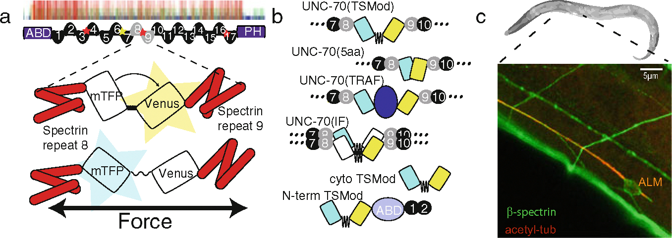
(a) Placement of TSMod between β-spectrin repeats 8 and 9 to generate a spectrin force sensor. Red stars indicate regions of high conformational flexibility [38]. (b) Suggested experimental and control constructs to validate and verify FRET values obtained from the protocol. From top to bottom: β-spectrin::TSMod force sensor; high FRET (5aa) and low FRET (TRAF) standards; intermolecular FRET control; soluble TSMod and terminal fusion as no-force control. (c) Expression of UNC-70::TSMod in adult C. elegans. A single ALM touch receptor neuron is highlighted by its coexpression of acetylated α-tubulin

1.2. Organization of the Protocol

We first begin the protocol with a brief description of the nematode Caenorhabditis elegans preparation for noninvasive imaging and a protocol to calibrate the collection efficiency of the photodetectors that is necessary to correct the FRET signal. The calibration also enables us to estimate individual pixel error with the aim to visualize these uncertainties in the final FRET map. We also implement an automatic neurite tracing algorithm, which tracks the boundary of the axon based on its Gaussian intensity distribution. We finally provide a detailed description of the analysis and the assessment of inter- vs. intramolecular energy transfer. This protocol is complemented by several excellent reviews dedicated to facilitate interpretation of the measurements [8, 39, 40].

2. Materials

2.1. Reagents and Consumables

1. Household bleach.

2. KOH.

3. NGM Agar plates seeded with Escherichia coli OP50.

4. Agarose.

5. Coverslips # 1.5.

6. Glass slides.

7. Immersion oil for microscopy (Leica; N = 1.513).

8. Optical lens cleaning paper (Thorlabs).

9. Windex.

10. Lab tape.

11. 0.1 μm latex beads, 2.5% w/v (PolySciences 00876–15).

12. Na₂HPO₄.

13. KH₂PO₄.

14. NH₄Cl.

15. NaCl.

16. NaOH.

17. Fluorescein isothiocyanate (FITC).

18. Ibidi 8-well microslide.

19. Distilled H₂O.

2.2. Equipment

1. Table top centrifuge.

2. Worm pick.

3. Stereoscopic dissecting microscope.

4. Laboratory glassware.

5. Leica SP5 confocal microscope with argon laser line for excitation of mTFP (458 nm) and Venus (514 nm) with single photon sensitive Hybrid (HyD) photodetectors (or other microscope equipped to visualize mTFP and Venus).

6. Vibration isolation table.

7. Glass slide holder.

8. 63× NA 1.4 or 100× NA 1.4 oil immersion objective.

9. 10× NA 0.5 air objective.

10. Excitation filter for GFP: 480 ± 20.

11. Emission filter for GFP 520 ± 20.

12. High performance image processing computer.

13. Epifluorescence light source.

2.3. Software

ImageJ; Python 3.10 (see https://gitlab.icfo.net/fret-analysis/fret-analysis).

2.4. Animal Strains

Described in Table 1.

Table 1.

Inventory of strains for mapping mechanical tension in neuronal spectrin cytoskeleton of living animals

Strain	Purpose	Genotype	Reference
GN517	TSMod	pgEx116 [unc-70 p::unc-70 (1–1166)::TSMod::unc-70 (1167–2267); myo-3 p::mCherry]	[12]
GN519	High FRET	pgEx131 [unc-70 p::unc-70 (1–1166)::mTFP-5aa-Venus:: unc-70 (1167–2267); unc-122 p::RFP]	[12]
GN600	No force	pgIs22 [unc-70 p::unc-70::TSMod]; oxIs95[pdi-2 p::unc-70 (fl); myo-2 p::GFP, lin-15] IV	[37]
MSB233/MSB366	Mutant	mirEx77 [unc-70 p::unc-70 (1–1166)::TSMod::unc-70 (1167–2267) E2008K; myo-2 p:mCherry]	[36]
MSB339	Low FRET	mirIs23 [unc-70 p::unc-70 (1–1166)::mTFP-TRAF-Venus:: unc-70 (1167–2267]; unc-70 (s1502); oxIs95[pdi-2 p:: unc-70 (fl); myo-2 p::GFP, lin-15] IV	[36]
GN498	Acceptor crosstalk	pgEx138[unc-70 p::unc-70 (1–1166)::TSMod (mTFPG73V)::unc-70 (1167–2267)::unc-54 utr, myo-2 p:: mCherry; unc-119 p::unc-119]	[12]
GN495	Donor bleedthrough	pgEx135 [unc-70 p::unc-70 (1–1166)::TSMod(G344V):: unc-70 (1167–2267)::unc-54 utr, myo-2 p::mCherry; unc-119 p::unc-119]	[12]
ARM101	Donor bleedthrough	wamSi101 [eft-3 p::mTFP::unc-54 3′UTR+ Cbr-unc-119 (+)]V.	[41]
GN493	Intermolecular	pgEx133[unc-70 p::unc-70 (1–1166)::TSMod (mTFPG73V]::unc-70 (1167–2267)::unc-54 utr;	[12]
	FRET	unc-70 p::unc-70 (1–1166)::TSMod(G344V)::unc-70 (1167– 2267)::unc-54 utr; myo-2 p::mCherry	[12]
GN566	Soluble TSMod	pgEx146[unc-70 p::TSMod::unc-54 utr]	[12]

2.5. Equipment Setup

2.5.1. Confocal Laser Scanning Microscope

A Leica SP5 II confocal scanning microscope is assembled around an upright Leica DMi6000 body equipped with an external epifluorescence illumination and GFP excitation and emission filters if dedicated mTFP and mVenus filters are not available. The microscope should be equipped with a holder for a glass slide, a 10× low magnification lens for searching the specimen and a high resolution 63×/1.4 or 100×/1.4 oil immersion objective for data acquisition. If the sample consists of mammalian neurons or other temperature-sensitive specimen, the microscope needs to be equipped with a temperature incubator. The confocal scanning system demands low noise GaAsP hybrid photodetectors with single photon sensitivity, a variable speed galvo scanner, and an argon laser with 458 and 514 nm laser lines. Spectral separation of the emission wavelength is best achieved with an acusto-optical beam splitter or a prism spectrometer detector. Alternatively, emission filters of 490 ± 30 nm for donor emission and 550 ± 30 nm for acceptor emission can be used in combination with a double band pass dichroic mirror (460/520 nm).

2.5.2. Standard Setup

1. Leica DMi6000 with external epifluorescence mercury arc or LED light source and corresponding filter sets.

2. Motorized Piezo z-stage for fast z-stacks.

3. HeNe 633 nm/10 mW, HeNe 594 nm/2.5 mW, HeNe 543/1.0 mW, Ar 458 nm/5 mW, 476 nm/5 mW, 488 nm/20 mW, 514 nm/20 mW or supercontinuum white light laser (covering wavelength from 450 to 590 nm).

4. Leica tandem scanner system.

5. Spectral detection module for adjustable spectral emission windows.

6. HC PL Fluotar 10×, air; HCX PL APO 63×/1.4 OIL.

7. Three standard fluorescent photomultiplier tubes (PMT) and two hybrid avalanche photodetectors (HyD).

8. Mounted on active vibration isolation.

3. Methods

3.1. Calibrating the Collection Efficiency of the Photodetector

Because the detection efficiency of common photodetectors varies with the wavelength of the photon, the linearity and collection efficiency of the hybrid GaAsP photodetectors have to be calibrated at least once for a given setup. Collection efficiency ψ_D and ψ_A can be determined experimentally by collecting photons from a homogeneous fluorescein solution with increasing gain at constant laser power (Fig. 2).

Fig. 2. Calibration of photodetector using a homogeneous FITC solution.

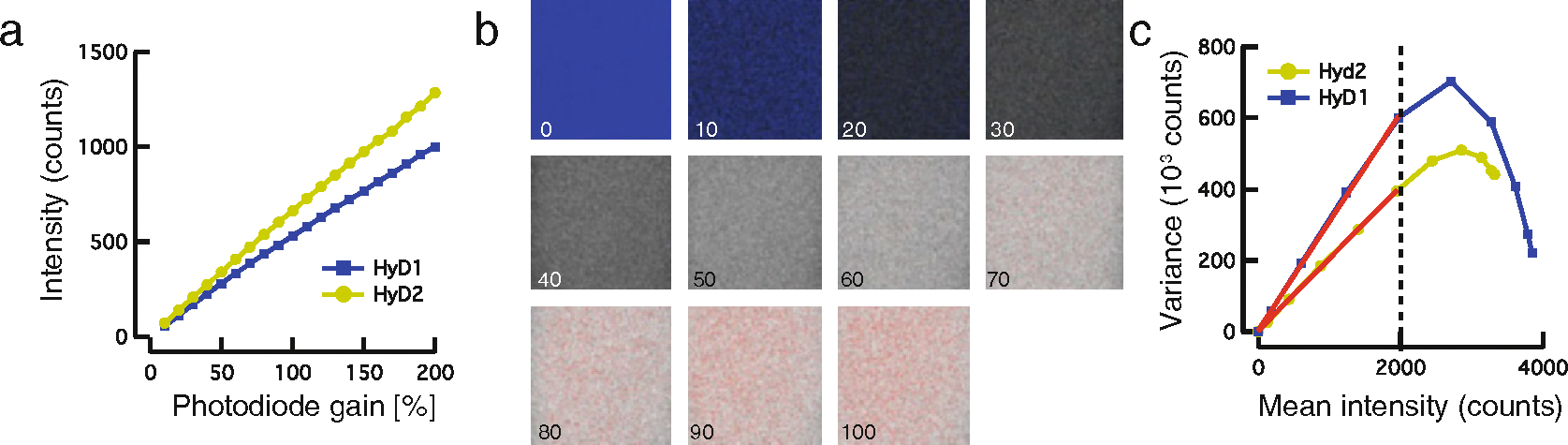
(a) Intensity counts plotted against increasing gain of each photodiode. Final settings were chosen in regions where the gain curves were perfectly linear, e.g., 150% for HyD1 and 100% for HyD2. (b) Representative images for the calibration in the HiLo lookup table highlighting oversaturated pixels in red. (c) Variance vs. mean intensity for a given ROI at increasing laser power. Laser power was adjusted in final imaging experiments to minimize saturated pixels. Standard deviation for each pixel as a function of intensity was determined from the line fit to the data. Roll-off above 2000 counts is due to pixel saturation. For a purely shot noise limited detection system a line is expected, hence fit range was limited between 0 and the dotted line

3.1.1. Determination of Collection Efficiency

• 1Prepare a 10% FITC solution in PBS.
• 2Make successive dilutions to obtain 1, 0.1, 0.01, 0.001% and pipette 30 μL of each dilution into a well of an ibidi “angiogenesis” μ-slide, which contains a coverslip bottom suitable for high-resolution imaging. Cover with an ibidi-cover and seal to prevent leakage of the dye-solution.
• 3Proceed to confocal microscope, add a drop of immersion oil on the coverslip and bring 63×/1.4 oil immersion lens into place.
• 4Start confocal microscope with the 488 nm line of a standard argon laser activated.
• 5In the configuration tab settings for the lasers, the argon laser should normally be set at 25% output power. Prolonged use of this laser at higher output powers will shorten its lifespan.
• 6Open the pinhole and adjust the prism spectrometer to between 500 and 600 nm emission wavelength.
• 7Adjust imaging parameters such that they are similar to those planned for biological samples, e.g., 1024 × 1024 pixels, 700 Hz linescan rate. Start with a low laser power, e.g., 10% transmission and adjust the gain to 10%.
• 8Collect an image and increase the gain successively until 200%.
• 9Repeat the same process with both hybrid GaAsP photodetectors.

3.1.2. Analysis

• 10Load each image into ImageJ or any other image analysis software.
• 11Draw a rectangular ROI in the center of the image and save it.
• 12Measure the mean pixel intensity and the standard deviation of the pixels in the ROI and repeat it for all images acquired.
• 13Plot the mean fluorescence against the gain for each photodetector (Fig. 2a).
• 14Select the gain for subsequent data acquisition for which the curve is linear. The steeper the curve, the more sensitive the diode. Select gains for which the mean fluorescence is similar. In our imaging system, the ideal gain was determined to be 100% for the acceptor diode and 150% for the donor diode.

3.1.3. Optional: Determination of Pixel Noise for Each Photodetector

• 1Prepare a 1% FITC solution in PBS and pipette 30 μL into ibidi u-slide. Cover with a coverslip to prevent leaking.
• 2Proceed to confocal microscope and add a drop of immersion oil on the coverslip and bring 63×/1.4 oil immersion lens into place.
• 3Start confocal microscope with the 488 nm line of a standard argon laser activated.
• 4Open the pinhole and adjust the spectral collection window between 500 and 600 nm emission wavelength.
• 5Adjust imaging parameters similar to the actual experiment, e.g., 1024 × 1024 pixels, 700 Hz linescan rate. Start with a low laser power, e.g., 0% transmission and adjust the optimal gain settings determine above for the donor and acceptor photodetectors, respectively.
• 6If collecting in photon counting mode, gain adjustment will be inactivated.
• 7Take an image and increase the laser power successively until 100% or pixels will start to saturate (see Note 1, Fig. 2b).
• 8Repeat the same process with both HyD photodetectors.

3.1.4. Analysis

• 9Load each image into ImageJ or any other image analysis software.
• 10Draw a rectangular ROI in the center of image and save it.
• 11Measure the mean pixel intensity and the standard deviation of the pixels in the ROI and repeat it for all images acquired (using the same ROI).
• 12Plot the variance of the pixel intensity of each ROI vs. the mean pixel intensity for each photodetector (Fig. 2c).
• 13Fit a line to the data and determine the y-intercept and the slope. The square-root of the slope is a measure for the standard deviation of each pixel, while the y-intercept is a measure for the dark current (see Note 2). If a significant number of pixels are saturated, the slope deviates from one for higher counts.

3.2. Age Synchronizing Animals Before Imaging

Keep animals using standard protocols and procedures as described in Ref. [42]. Because mechanical tension is subject to cellular regulation and might depend on animal size, developmental stage, and age, only animals from an age-synchronized population should be imaged.

• 1Prepare bleaching solution by combining 0.2 mL household bleach (stored in an opaque or brown glass container), 20 μL 5 M KOH, and 0.8 mL H₂O to obtain 1 mL bleaching solution. Prepare always fresh bleach stock before the experiment and change it every couple of months since it is not stable.
• 2Prepare M9 buffer: add 6 g Na₂HPO₄; 3 g KH₂PO₄; 1 g NH₄Cl; 0.5 g NaCl, adjust the volume to 1 L with H₂O and autoclave.
• 3Wash worms off from a 6 cm plate using 1 mL M9 buffer (or filtered ddH₂O) and transfer onto a 1.5 mL microcentrifuge tube.
• 4Spin down worms for 20 s at 1200 rpm.
• 5Optional: Discard supernatant and repeat the wash three times until no bacteria or other contaminants are visible in the supernatant.
• 6Resuspend the worms in 1 mL bleaching solution and incubate for 5 min or until most of the adult worms break apart and release their eggs into the solution (see Note 3).
• 7Pellet carcasses and eggs by spinning for 1 min at 150–200 rpm.
• 8Remove supernatant and wash 3 times with M9 buffer.
• 9Add 20 μL of M9 and pipette the eggs onto a new agar plate containing a lawn of E. coli OP50.
• 10Check after 60 h growth at 20 °C and use young adult worms or any age for imaging.

3.3. Mounting Animals for Imaging

Young adult animals or any other age-synchronized stage can be mounted in various ways [43–50] and in different body positions [36, 50, 51]. For the sake of simplicity, we follow here the simple agar pad compressive immobilization with latex beads [12, 43].

• 11Prepare a 6% agarose solution in M9 and dissolve by heating in a microwave.
• 12Meanwhile, prepare two glass slides with a “spacer-tape” adhered on top of them (see Fig. 3). Bring a third glass slide between them. Pipette a drop (50–100 μL) of dissolved agar solution on the middle glass slide and immediately compress the drop with a glass slide. The adhesive tape of the two bordering glass slides will act as a spacer and hence ensure a constant thickness of the agar pad. Store in a humidified chamber to prevent drying and use immediately (see Note 4).
• 13Take a glass slide with an agar pad and pipette 2 μL of latex bead solution onto the middle of the agar pad.
• 14Pick brightly fluorescing young adult worms under a stereo microscope into the drop.
• 15Cover gently with a glass coverslip and proceed immediately to imaging (see Note 5).

Fig. 3. Preparation of the agar pad.

One glass slide is sandwiched between two slides that are modified with lab tape that acts as a spacer. A drop of agar solution is pipetted on top of the middle slide and compressed with another slide to create a flat bed of agar. A droplet of latex beads is pipetted on top of the pad, in which the worms are deposited with a worm pick. The droplet with the worms is covered with a glass coverslip #1.5 thickness

3.4. Imaging

Critical:

The following procedure is optimized for a Leica SP5 point scanning confocal setup described above. If an alternative setup is used, it will be necessary to modify relevant parameters (such as emission filter band, excitation laser intensity, and scan line rate) to achieve the best resolution and FRET signal.

• 1Proceed to the microscope immediately after mounting the worms. Prevent drying of the agar pad by keeping it in a humidified chamber. Caution! Drying will increase the salt content and therefore perturb the worms osmotically and lead to dehydration.
• 2Look for the worms with a low magnification objective (10× air) and bring into the center of the field of view.
• 3Place a drop of immersion oil on top of the coverslip and change to the 63×/1.4 oil immersion lens.
• 4Using an attached epifluorescence lamp, observe worms through widefield fluorescence by illuminating with any standard GFP excitation and emission filter, identify the region of interest, and bring the animal into focus (see Note 6).
• 5Switch to confocal mode and select imaging parameter according to step 11. Three different images need to be acquired to gain access to the FRET signal using sensitized emission. Four additional images are needed to eliminate spectral contamination (donor bleedthrough and acceptor crosstalk) from the raw FRET intensity image.
• 6Define a sequential scan to take the donor and acceptor images sequentially and minimize spectral contamination. The sequential scans will have only one laser active at a time while collecting photons in both the mTFP and Venus channels.
• 7Choose 1024 × 1024 pixels to obtain adequate resolution and adjust the zoom so that the pixel size of the image does not cause over- or undersampling. For optimal sampling, see Note 7.
• 8Select the 458 and 514 nm lines of continuous wave argon ion laser to excite the mTFP and Venus fluorophores, respectively. Start with a low laser power and increase if the signal is too poor, e.g., 50% for the donor (≈6 μW) and 11% for the acceptor excitation (≈4 μW). For reproducible measurements, the incident power of the excitation light should be measured with a Thorlabs microscope slide power meter head (S170C) attached to PM101A power meter console.
• 9Select bit depth of 16 (preferred) or 12 (adequate) to obtain 64,000 or 4096 gray levels, respectively. Importantly, do not excede these intensities since FRET values cannot be derived from saturated pixels (see Note 1).
• 10Activate two HyD photodetectors and set the emission bandwidth using the prism spectrometer detector to 465–500 nm for the donor channel and 520–570 nm for the acceptor channel.
• 11Adjust detector gain of the donor photodiode to 150% and acceptor detector gain to 100%. Gains need to be set according to the calibration to achieve equal collection efficiency (see above). Calibration of the detectors ensures similar collection efficiency under preset gain setting (see Note 8).
• 12Find the animal in “live” mode only in the acceptor channel and choose appropriate zoom level matching optimal sampling (see Note 7). Reducing the imaging time and power in the acceptor channel avoids unnecessary bleaching of the rather labile mTFP donor fluorophore.

Optional to reduce imaging noise: perform 4× line averaging during acquisition.

• 13Switch to line-by-line scan for the final image acquisition. This minimizes motion artefacts and ensure that donor and acceptor pixels match perfectly.
• 14Capture four images under the following conditions (see Note 9):

  1. Donor excitation → Donor emission = I_D → Donor channel.

     Ex 458 nm.

     Em 465–500 nm

  2. Donor excitation → Acceptor emission = I_F → FRET channel.

     Ex 458 nm.

     Em 520–570 nm

  3. Acceptor excitation → Acceptor emission = I_A → Acceptor channel.

     Ex 514 nm.

     Em 520–570 nm

  • (X)Acceptor excitation → Donor emission (This channel does not contain any information and can be discarded).

    Ex 514 nm.

    Em 465–500 nm

• 15Save them appropriately and proceed to bleedthrough estimation.

3.4.1. Quantifying Spectral Contaminants (Bleedthrough, Crosstalk)

Intensity-based FRET imaging is prone to spectral bleedthrough and crosstalk between individual channels due to the overlapping fluorescence spectra of the donor and acceptor chromophores. Acceptor crosstalk is defined as the direct excitation of the acceptor fluorophore by the donor laser line (Fig. 4a–i). Donor bleedthrough is defined as the donor emission in the FRET channel after direct donor excitation, in the absence of an acceptor (Fig. 4a–ii). Several methods have been introduced that rely on constant or varying correction factors [53–55]. Critically, determination of the bleedthrough factors has to be performed for each experiment. It is not sufficient to do it once for a given setup, especially if imaging parameters such as photodetector gain, laser power, and detection bandwidth are changed during an experiment to improve imaging conditions (see Note 8).

1. Immobilize a sample that contains just the donor fluorophore, e.g., ARM101 is a worm that expresses only the mTFP [41].

2. Take two images after direct excitation of the donor and recording the emission in the donor and the FRET channels to get access to I_D and I_F, respectively.

   1. Donor excitation → Donor emission = I_D → Donor channel

      Ex 458 nm

      Em 465–500 nm.

   2. Donor excitation → Acceptor emission = I_F → FRET channel

      Ex 458 nm

      Em 520–570 nm

3. Immobilize a worm that expresses only the acceptor fluorophore, e.g., GN498 is a worm that only expresses mVenus [12].

   1. Donor excitation → Acceptor emission = I_F → FRET channel

      Ex 458 nm

      Em 520–570 nm

   2. Acceptor excitation → Acceptor emission = I_A → Acceptor channel

      Ex 514 nm

      Em 520–570 nm

Fig. 4. Determining the spectral contamination in the FRET channel.

(a) Schematic of the single fluorophore construct to determine spectral crosstalk. (i) Spectral situation of the FRET experiment in the absence of the donor. Residual excitation of the acceptor with the 458 nm line leads to detectable emission in the FRET channel. (ii) Spectral situation of the FRET experiment in the absence of the acceptor. The long-tailed emission of the donor leads to significant signal in the FRET channel. Red line indicates the varying collection efficiency of the photodetector; gray squares represent collection band determined by the spectral detectors; black peaks indicate the two laser lines. Spectra assembled with fpbase.org [52]. (b–d) Panel of different imaging controls characterizing spectral contamination in the imaging channels. The fluorescent probe consists of either the acceptor (upper row) or the donor (lower row). (b) Representative images of the acceptor emission after direct acceptor excitation for the two control constructs. (c) Representative images of the acceptor emission after donor excitation for the two different controls. (d) Representative images of the donor channel after direct excitation of the donor. The white square indicates the ROI to extract the signal from either spectral contamination in the FRET channel. (e) Distribution of bleedthrough factors acquired over the course of 2 years. Red point = median ± confidence interval on the median

3.5. Analysis

In the following section we provide a detailed description of the FRET analysis protocol and its accompanying analysis scheme (Fig. 5). For the convenience of the experimenter, a Python code with all steps is available under this link, which has been adapted from the original protocol in Ref. [12]. The program contains three modules, one module for the bleedthrough determination (Fig. 5, Module 1) and two modules for the FRET data processing (Fig. 5, Modules 2 and 3). Module 2 elaborates an automated neurite tracing and local background subtraction to determine the FRET efficiency in neurons. This module has advantages for FRET calculation in vivo with spatial varying background fluorescence, e.g., in the nematode. Alternatively, if the ROI is an irregular object, Module 3 provides the user with a manual ROI selection for global background subtraction (Fig. 5). In general, to obtain the FRET values from the recorded data, the following steps need to be performed.

Fig. 5. Overview of the analysis with flowchart.

(1) Bleedthrough determination and FRET processing are done on separate sets of images. Bleedthrough factors were loaded into the main program. (2–6) Representative steps in the flow of the FRET calculation

(2) Load images

(3) Global or local background subtraction of a moving window after Gaussian fit to the neurite intensity profile. Simultaneous determination of ROI boundaries from the width of the fit

(4) Bleedthrough correction

A python code with the three modules and detailed instructions is available under https://gitlab.icfo.net/fret-analysis/fret-analysis

1. Determine the spectral bleedthrough factors

To correct for spectral contamination in the FRET channel from donor bleedthrough and acceptor cross excitation, the intensity in the FRET channel is divided by the corresponding intensity of the directly illuminated channel, which gives rise to the bleedthrough ratios.

1. Load the bleedthrough images into ImageJ or any equivalent image processing program.

2. Select an ROI containing a region with strong but not saturated fluorescent signal in the image pair and select an ROI with background fluorescent (white and orange squares, respectively, in Fig. 4b–d).

3. Quantify the mean signal in each ROI.

4. Subtract the mean background intensity (e.g., from the orange square) and the “signal” intensity (e.g., from the white square) in the image pairs as indicated in Fig. 4.

5. Calculate the bleedthrough ratio of the donor and acceptor channels ($\delta$ and $\alpha$) according to:

   $$\delta =\frac{\sum \frac{I_F(x,y)}{I_{D(x,y)}}}{N}\text{and}\alpha =\frac{\sum \frac{I_F(x,y)}{I_{A(x,y)}}}{N}$$

   with $N$ as the number of pixels (with the coordinate $x,y$) in the ROI, $I_F$ is the intensity value in the “FRET” channel (acceptor emission after donor excitation, Fig. 4b), and $I_A$ and $I_D$ are the intensity in the acceptor and donor channel (after direct excitation, Fig. 4a, c), respectively.

6. Keep $\alpha$ and $\delta$ for the linear unmixing.

2. Local background subtraction and neurite tracing

The width of most neurons in C. elegans approaches the diffraction limit (200–300 nm in diameter) and therefore is a convolution of the Gaussian intensity distribution of the point spread function of the imaging system (Fig. 6a–i). The extension of the neuron, however, spans many hundreds of micrometers in length. Therefore, background fluorescence is not constant and regional variation exists along the length of the neuron through the animal’s body (Fig. 6a–i, b, c). To accommodate these special needs, we perform a local background subtraction at each position in the image after fitting the raw intensity profile to a single Gaussian and subtracting the baseline fit parameter $I_0$ at that position.

1. Load image stack containing all three channels into your favorite image processing software (e.g., Fiji/ImageJ) (Fig. 7a–c).

2. Select the neuron of interest with the 20–30 pixel wide segmented line tool and straighten the ROI (Edit > Selection > Straighten). Save selected ROI for reference.

3. Save the straightened image stack.

4. Import into data analysis program to determine the ROI selection through iterative-fitting procedures.

5. Fit a Gaussian to the intensity profile (Fig. 6a–ii), column by column for each channel separately:

   $$I(x,y)=I_0+{\left.A\cdot \mathrm{e}\mathrm{x}\mathrm{p}\left({\left(-\frac{x-x_0}{\sigma }\right)}^2\right)\right|}_y$$

6. Keep width $\sigma$ of the Gaussian to define the ROI for final calculation of FRET efficiency, E (white line in Fig. 6a–iii). Hence, we restrict the final calculation of the FRET efficiency to the pixels which fall into the range of the intensity distribution of the acceptor channel according to $E(x,y){\in }_{x0}(x,y)\pm \sigma (x,y)$. For segmentation and shape analyses, the fit also determines the centerline of the ROI, $x_0$.

7. Subtract the $I_0$, the local background, from each corresponding column:

   $$I_D;I_A;I_F(x,y)=I(x)-{\left.I_0\right|}_y$$

Fig. 6. Background subtraction and neurite tracing.

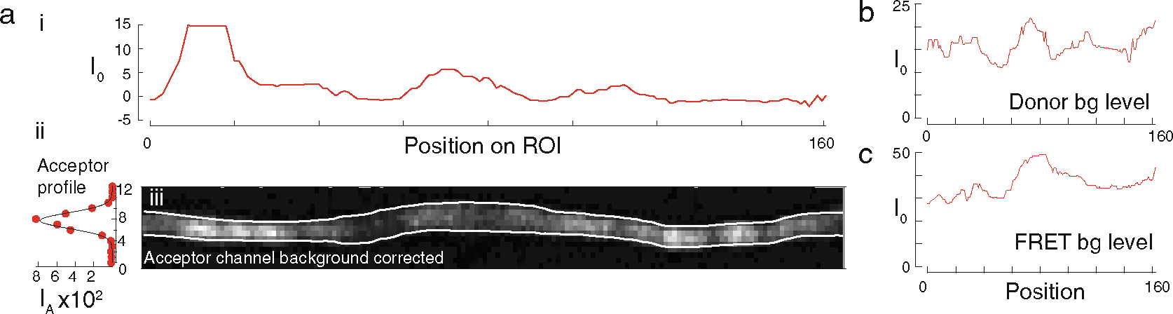
(a) Representative background subtraction of a neurite in the acceptor channel after direct excitation of the acceptor. (i) The background level is shown for each row of pixels in the image. (ii) Gaussian distribution of the intensity at a certain pixel position after background subtraction. (iii) Background subtracted acceptor channel intensity image. White lines indicate boundaries of the ROI found by our fitting procedure. (b) Background level of the same ROI of the donor channel and (c) the raw FRET channel

Fig. 7. Representative results from UNC-70 β-spectrin::TSMod and control constructs.

(a) Donor fluorescence after direct excitation. (b) Acceptor fluorescence after direct excitation. (c) Acceptor fluorescence after donor excitation (uncorrected FRET signal). (d) Processed and corrected FRET efficiency maps of representative axonal ROIs. (e) Summary of the observed FRET efficiencies derived from the individual constructs. (f) Plot of the FRET efficiency against the acceptor intensity indicates that most FRET is due to intramolecular transfer

3. FRET calculation

1. Use the empirically determined bleedthrough factors, $\alpha$ and $\delta$, from Subheading 3.4.1 to calculate the bleedthrough corrected FRET signal from background subtracted intensities in the FRET, donor, and acceptor channels on a pixel-by-pixel basis according to.

   $$\mathrm{c}\mathrm{F}(x,y)=I_F(x,y)-\delta \cdot I_D(x,y)-\alpha \cdot I_A(x,y)$$

   with $cF(x,y)$ as the corrected FRETsignal at a certain pixel coordinate $x,y,I_F(x,y)$ as the raw, background subtracted FRET intensity, $I_D(x,y)$ as the background subtracted donor intensity, and $I_A(x,y)$ as the background subtracted acceptor intensity.
2. Calculate the FRET efficiency within the neurite boundaries determined above according to [32]:

   $$\begin{gathered} E=\frac{\mathrm{c}\mathrm{F}}{I_D+\mathrm{c}\mathrm{F}} \\ E=100\times \left(\frac{\left(\mathrm{c}\mathrm{F}\cdot Q_D\cdot \frac{D}{A}\right)}{\mathrm{q}\mathrm{D}+\left(\mathrm{c}\mathrm{F}\cdot Q_D\cdot \frac{D}{A}\right)}\right) \end{gathered}$$

   with $I_D$ being the donor and bleedthrough corrected FRET channel intensities, respectively, $Q_D$ as the previously determined donor quantum yield [33], qD and cF are the (quenched) donor emission (in the presence of acceptor) and bleedthrough corrected FRET emission, respectively, and the ratio D/A is the collection efficiency/gain ratio of the donor and acceptor photodetector as experimentally determined in Subheading 3.1.

3. For each neuron, calculate an average FRET value and repeat this analysis for several samples taken from multiple animals. The number of samples needed to detect an effect of a treatment or genetic perturbation will depend on the variance in the biological control samples and the expected effect size.

4. Repeat this analysis for different imaging control constructs with FRET pairs connected by varying linker length or a “no-force control” (Fig. 1b). A constitutively high FRET construct was engineered by replacing the entropic spring in TSMod by a 5 amino acid linker or a large domain (TRAF domain) that separate the two fretting fluorescent proteins [12, 33, 56] (see Note 10).

5. All FRET efficiency values obtained from the force-sensitive TSMod cassette should fall into the dynamic range delineated by the low and high FRET standards (Fig. 7e). In our case, we measured an average FRET value of 22% for the experimental β-spectrin::TSMod construct, whereas the “no-force control,” a TSMod without linkers expressed in the cytoplasm, showed an average FRET efficiency of 38%. If the average TSMod FRET is lower than the average of the no-force control construct, the difference indicates the amount of force by which the host protein is under tension (for representative results, interpretation, and more imaging tips to prevent artefacts, see Notes 11–19).

4. Optional: Error analysis and estimating the uncertainty of the FRET calculation

One of the drawbacks of FRET is poor signal-to-noise metrics, especially at low photon counts [57]. To visualize the certainty or uncertainty of the FRET calculation (Fig. 8a–d), we can estimate the error for each pixel inside the region of interest (Fig. 8c). The error for FRET calculation for each pixel can be propagated from the empirically determined pixel error in each channel according to

$$\begin{gathered} {\sigma }_{\mathrm{c}\mathrm{F}}(x,y)=\frac{1}{\sqrt{N}} \\ \times \sqrt{({\left(I_F(x,y)\cdot {\sigma }_F\right)}^2+{\left(I_D(x,y)\cdot {\sigma }_D\right)}^2+{\left(I_A(x,y)\cdot {\sigma }_A\right)}^2)} \end{gathered}$$

$$\begin{gathered} {\sigma }_E(x,y)={\left(\frac{E}{\mathrm{c}\mathrm{F}(x,y)}\right)}^2\cdot \frac{1}{\sqrt{N}} \\ \times \sqrt{{\left(\mathrm{c}\mathrm{F}(x,y)\cdot {\sigma }_D\right)}^2+{\left(I_D(x,y)\cdot {\sigma }_{\mathrm{c}\mathrm{F}}\right)}^2} \end{gathered}$$

where $N$ is the number of measurements for each pixel; ${\sigma }_F,{\sigma }_A$, ${\sigma }_D$ are standard deviation of each pixel in the FRET, acceptor, and donor channel (Fig. 8a–c), respectively (as experimentally determined in Subheading 3.1); ${\sigma }_{cF}$ is standard deviation of spectrally corrected FRET channel; and ${\sigma }_E$ is the standard deviation of the value for FRET in each single pixel, assuming complete independence of noise in the donor and acceptor detectors. Both detectors follow Poisson statistics and variance scales linearly with number of photons counted as tested experimentally (Fig. 2c). We found that pixels with low acceptor signal (e.g., outside the ROI) have a high uncertainty in the FRET channel (Fig. 8e) (see Note 20).

Fig. 8. FRET and error calculation.

(a) Pseudocolored FRET channel intensity image after bleedthrough correction and background subtraction. Same ROI as in Fig. 6. (b) FRET efficiency image after FRET calculation of all pixels within the fitted ROI boundaries. (c) Corresponding uncertainty image of all pixels including the pixels outside the fitted ROI. Red pixels highlight the ones with a high error and are excluded from the statistics. (d) Average FRET efficiency as a function of neurite position. (e) Uncertainty of the FRET calculation plotted against the acceptor intensity indicates that the largest error is expected for pixels with a low molecular representation. Further analysis shows that the large errors occur outside the respective ROIs

4. Notes

1. Important for all image acquisition steps. Do not saturate pixels since this causes a deviation from linearity in the response. Reduce laser power during the image acquisition such that pixels are never saturated. Check with HiLo palette if necessary.

2. Avalanche photodiodes and hybrid GaAsP (HyD) detectors can be operated in photon counting mode with all gains on the detection disabled. If possible, repeat the calibration in photon counting mode. Such an analysis should reveal a slope of one, expected for shot noise limited detectors like these that follow Poisson statistics.

3. The egg shell is bleach resistant and therefore embryos can be easily isolated using this procedure. Over-incubation, however, may result in damage to some eggs, reducing the yield of age-synchronized animals.

4. High-percentage agarose is needed to completely immobilize the worm. If lower percentage agarose is used, e.g., 2%, the worm will be able to move and eventually crawl out of the field of view. Alternatively, when using 2% agarose, worms can be anesthetized by adding 1 μL of 1 mM levamisole onto the pad prior transferring the animals.

5. The compressive immobilization method in a high-percentage agarose might alter mechanical behavior of the animal. If neither high-percentage agarose nor anesthetics can be used, microfluidic devices have specifically been engineered to trap living animals for imaging [49, 58, 59].

6. Microscopy facilities often do not have the optimal filter combinations for mTFP and Venus in the widefield epi-illumination pathway. In our experience, however, specialized mTFP or Venus filters are not required to see these fluorophores. Take care to limit the illumination time and power to prevent accidental bleaching of the fluorophores before actually acquiring data.

7. Because confocal imaging is a process of converting a continuous space signal into a numeric sequence, it is subjected to artefacts based on the sampling rate. The Nyquist theorem suggests that sampling of an analog signal should be carried out at the Nyquist rate, which is twice the fundamental frequency of the expected signal. In the confocal microscope, the highest fundamental frequency to be recorded is imposed by the optical system and is set by the resolution of the objective and particular wavelength to be imaged [60]. According to Nyquist theorem, the pixel size therefore has an optimum at p < r/2.3, with r as the smallest resolvable structure (e.g., the diffraction limit). A much smaller pixel size leads to unnecessary bleaching without additional gain in information.

8. Always keep the laser power and photodetector settings constant during an experiment. If parameters have to be varied, be sure to acquire bleedthrough images at the exact same imaging conditions (Fig. 4e) to eliminate cross excitation of the fluorophores due to the overlapping excitation spectra.

9. Make sure that the two channels are spatially well aligned. This is particularly important for camera-based detection and image splitting optics. Such pixel shift needs to be meticulously corrected for with submicron beads and post-acquisition image processing [34].

10. The bleedthrough ratios are generally assumed to be constant for all images taken with the same microscope setting and laser power. Therefore, the fraction of the donor and acceptor fluorescence in the raw FRET signal was subtracted. Even though the assumption of a constant bleedthrough ratio is generally valid, photon arrival rate can also be modeled as a Poisson process in which the bleedthrough ratio might not be constant but depend on the actual pixel intensity of the directly illuminated channel. These phenomena play an important role when FRET is based on photon counting and hence signal-to-noise ratio approaches its limits. In such a case, the bleedthrough ratio can be modeled as a single exponential.

11. The comparison of the TSMod construct with the proposed FRET standards provide a reliable means to deduce quantitative values from intensity-based FRET imaging. Since the high FRET (5aa) and low FRET (TRAF) control standards have a fixed linker length and therefore have FRET efficiencies that do not vary with the mechanical state of the host protein. Likewise, the FRET values obtained from these constructs should not change upon different experimental conditions, e.g., drug treatment or mechanical manipulation. Previously, the FRET efficiency of both constructs was quantified by FLI microscopy and determined to be 50% and 10%, respectively [12, 33]. Even though the values derived from these standards can vary depending on the experimental system and specific FRET calculation, any experimental values falling outside of this dynamic range delineated by the fixed length FRET sensors should be treated with caution.

12. Dynamic measurement may be used, whenever possible, to manipulate the molecular tension while reading out FRET signals in real time. In that case, the FRET reporter can be assessed to which degree it is able to report a mechanical stress during a physiological process. For example, if no change of FRET occurs despite an imposed cellular strain, internal force transmission pathways might be disrupted. To a rough approximation, 5% difference in average FRET values correspond to ≈1.5 pN of tensile load. A detailed description of the calibration and design of different TSMod variants can be found in Refs. [10, 24].

13. In some circumstances, FRET values of the TSMod can be larger than the relaxed or no-force controls [20, 36]. Not all host molecules need to be under tension and several reports indicate the TSMod can also report whether or not the host proteins are under compression. Glycocalyx proteins experience significant compression during cellular adhesion [20], and β-spectrin is a flexible molecule that can sustain tensile and compressive stresses, depending on the physiological context and the animal’s locomotory activity [36].

14. Pitfall: Intermolecular FRET.

    Several factors can make the interpretation of the FRET values challenging. For instance, intermolecular FRET may occur if the TSMod-expressing transgene is over-expressed, which would preclude the force measurements. A straightforward way to probe for the occurrence of intermolecular FRET is to generate doubly transgenic cells or animals in which two different molecules are expressed with either the acceptor or donor fluorophores silenced. Such constructs can be generated by mutating the conserved glycine residue to valine in each fluorophore (Table 1 and [12]). Any significant FRET signal in this transgenic must come from intermolecular FRET (Fig. 7d, e), as no FRET pair exists within the same molecule. Alternatively, if such constructs are not available, the calculated FRET efficiency can be related to the emission intensity of the acceptor channel after direct excitation of the acceptor (Fig. 7f). Under first approximation, this serves as a proxy for protein concentration [61].

15. Pitfall: Autofluorescence.

    Autofluorescence is a common problem when imaging in living tissues. C. elegans is known to express a high density of autofluorescent and birefringent vesicles in the intestine [62]. Several mutations of the glo genes interfere with the formation of the gut granules and thus lead to a strong reduction of the autofluorescence [62]. If using a genetic intervention is not possible because these genes also interfere with processes that are important for the question under investigation, fluorescence lifetime imaging microscopy can be used to decipher signal that originates from specific and nonspecific fluorophores. Autofluorescent dyes have a much shorter excited state lifetime (<1 ns) than genetically encoded fluorescent proteins (>>1 ns) such that pixels with this contribution can be easily distinguished [12, 63].

16. The current force sensors are built with standard fluorescent proteins well-matched to the reducing environment of the cytoplasm. These sensors might not work as well in extracellular milieu, under strongly oxidizing conditions. To improve force sensors enabling the visualization of stresses in the extracellular matrix, fluorescent proteins optimized for specific cellular environments could be used [64, 65].

17. Even though molecular tension sensors report on the average force per molecule, it represents a bulk measurement, as many molecules within a single pixel measurement contribute to the signal. Thus, individual molecules might experience more or less tension or even be compressed within the imaged volume. As pointed out before [8], the obtained FRET values are also averaged over the acquisition time and, especially, for scanning confocal represents a tiny snapshot within the image. This is even more prevalent in FLI microscopy, which may require tens of seconds to collect enough photons for subsequent fitting routines [33].

18. Sensitized emission FRET can produce known and characterized artefacts, e.g., associated with spectral bleedthrough or differential bleaching of the donor/acceptor fluorophores during the acquisition time. Other methods are available that minimize the impact of these issues, e.g., FLIM-FRET [12, 63], acceptor photobleaching [15], and spectral imaging [66].

19. If FRET values are notoriously high or negative, check bleedthrough constants and/or reevaluate the background subtraction.

20. For low signal, a high uncertainty is expected, as seen in Fig. 8e. Mostly, these pixels fall outside the ROI and can be excluded.

References

- 1.Kung C (2005) A possible unifying principle for mechanosensation. Nature 436(7051):647–654 [DOI] [PubMed] [Google Scholar]
- 2.Katta S, Krieg M, Goodman MB (2015) Feeling force: physical and physiological principles enabling sensory mechanotransduction. Annu Rev Cell Dev Biol 31(1):347–371. 10.1146/annurev-cellbio-100913-013426 [DOI] [PubMed] [Google Scholar]
- 3.Venturini V, Pezzano F, Castro FC et al. (2020) The nucleus measures shape changes for cellular proprioception to control dynamic cell behavior. Science 370(6514). 10.1126/science.aba2644 [DOI] [PubMed] [Google Scholar]
- 4.Hoffman BD, Grashoff C, Schwartz MA (2011) Dynamic molecular processes mediate cellular mechanotransduction. Nature 475(7356):316–323 [DOI] [PMC free article] [PubMed] [Google Scholar]
- 5.Krieg M, Dunn AR, Goodman MB (2015) Mechanical systems biology of C. elegans touch sensation. BioEssays 37(3):335–344. 10.1002/bies.201400154 [DOI] [PMC free article] [PubMed] [Google Scholar]
- 6.Krieg M, Fläschner G, Alsteens D et al. (2018) Atomic force microscopy-based mechanobiology. Nat Rev Phys 1:41–57. 10.1038/s42254-018-0001-7 [DOI] [Google Scholar]
- 7.Castro F, Venturini V, Ortiz-V’asquez S et al. (2021) Direct force measurements of subcellular mechanics in confinement using optical tweezers. J Vis Exp 2021(174):1–35. 10.3791/62865 [DOI] [PubMed] [Google Scholar]
- 8.Gayrard C, Borghi N (2016) FRET-based molecular tension microscopy. Methods 94(2016):33–42. 10.1016/j.ymeth.2015.07.010 [DOI] [PubMed] [Google Scholar]
- 9.Hurst S, Vos BE, Brandt M et al. (2021) Intracellular softening and increased viscoelastic fluidity during division. Nat Phys 17(11):1270–1276. 10.1038/s41567-021-01368-z [DOI] [Google Scholar]
- 10.Grashoff C, Hoffman BD, Brenner MD et al. (2010) Measuring mechanical tension across vinculin reveals regulation of focal adhesion dynamics. Nature 466(7303):263–266 [DOI] [PMC free article] [PubMed] [Google Scholar]
- 11.Canever H, Carollo PS, Fleurisson R et al. (2021) Molecular tension microscopy of E-Cadherin during epithelial- mesenchymal transition. Methods Mol Biol 2179:289–299 [DOI] [PubMed] [Google Scholar]
- 12.Krieg M, Dunn AR, Goodman MB (2014) Mechanical control of the sense of touch by β-spectrin. Nat Cell Biol 16(3):224–233. 10.1038/ncb2915 [DOI] [PMC free article] [PubMed] [Google Scholar]
- 13.Cai D, Chen SC, Prasad M et al. (2014) Mechanical feedback through E-cadherin promotes direction sensing during collective cell migration. Cell 157(5):1146–1159. 10.1016/j.cell.2014.03.045 [DOI] [PMC free article] [PubMed] [Google Scholar]
- 14.Vuong-Brender TTK, Boutillon A, Rodriguez D et al. (2018) HMP-1/ α-catenin pro- motes junctional mechanical integrity during morphogenesis. PLoS ONE 13(2):1–21. 10.1371/journal.pone.0193279 [DOI] [PMC free article] [PubMed] [Google Scholar]
- 15.Ye AA, Cane S, Maresca TJ (2016) Chromosome biorientation produces hundreds of piconewtons at a metazoan kinetochore. Nat Commun 7:1–9. 10.1038/ncomms13221 [DOI] [PMC free article] [PubMed] [Google Scholar]
- 16.Lemke SB, Weidemann T, Cost AL et al. (2018) A small proportion of Talin molecules transmit forces to achieve muscle attachment in vivo. PLoS Biol 310(939):446336. 10.1101/446336 [DOI] [PMC free article] [PubMed] [Google Scholar]
- 17.Conway DDE, Breckenridge MMT, Hinde E et al. (2013) Fluid shear stress on endothelial cells modulates mechanical tension across VE-cadherin and PECAM-1. Curr Biol 23(11):1024–1030. 10.1016/j.cub.2013.04.049.Fluid [DOI] [PMC free article] [PubMed] [Google Scholar]
- 18.Aird EJ, Tompkins KJ, Ramirez MP et al. (2020) Enhanced molecular tension sensor based on Bioluminescence Resonance Energy Transfer (BRET). ACS Sensors 5(1):34–39. 10.1021/acssensors.9b00796 [DOI] [PMC free article] [PubMed] [Google Scholar]
- 19.Ringer P, Weißl A, Cost AL et al. (2017) Multiplexing molecular tension sensors reveals piconewton force gradient across talin-1. Nat Methods 14(11):1090–1096. 10.1038/nmeth.4431 [DOI] [PubMed] [Google Scholar]
- 20.Paszek MJ, DuFort CC, Rossier O et al. (2014) The cancer glycocalyx mechanically primes integrin-mediated growth and survival. Nature 511(7509):319–325 [DOI] [PMC free article] [PubMed] [Google Scholar]
- 21.Guo J, Wang Y, Sachs F et al. (2014) Actin stress in cell reprogramming. Proc Natl Acad Sci 111(49):E5252–E5261. 10.1073/pnas.1411683111 [DOI] [PMC free article] [PubMed] [Google Scholar]
- 22.Meng F, Suchyna TM, Sachs F (2008) A fluorescence energy transfer-based mechanical stress sensor for specific proteins in situ. FEBS J 275(12):3072–3087 [DOI] [PMC free article] [PubMed] [Google Scholar]
- 23.Ye N, Verma D, Meng F et al. (2014) Direct observation of α-actinin tension and recruitment at focal adhesions during contact growth. Exp Cell Res 327(1):57–67. 10.1016/j.yexcr.2014.07.026 [DOI] [PMC free article] [PubMed] [Google Scholar]
- 24.LaCroix AS, Lynch AD, Berginski ME et al. (2018) Tunable molecular tension sensors reveal extension-based control of vinculin loading. elife 7:1–36. 10.7554/elife.33927 [DOI] [PMC free article] [PubMed] [Google Scholar]
- 25.Arsenovic PT, Ramachandran I, Bathula K et al. (2016) Nesprin-2G, a component of the nuclear LINC complex, is subject to myosindependent tension. Biophys J 110(1):34–43. 10.1016/j.bpj.2015.11.014 [DOI] [PMC free article] [PubMed] [Google Scholar]
- 26.Dejardin T, Carollo PS, Sipieter F et al. (2020) Nesprins are mechanotransducers that discriminate epithelial-mesenchymal transition programs. J Cell Biol 219(10). 10.1083/JCB.201908036 [DOI] [PMC free article] [PubMed] [Google Scholar]
- 27.Borghi N, Sorokina M, Shcherbakova OG et al. (2012) E-cadherin is under constitutive actomyosin-generated tension that is increased at cell-cell contacts upon externally applied stretch. Proc Natl Acad Sci U S A 109(31):12568–12,573 [DOI] [PMC free article] [PubMed] [Google Scholar]
- 28.Price AJ, Cost AL, Ungewiß H et al. (2018) Mechanical loading of desmosomes depends on the magnitude and orientation of external stress. Nat Commun 9(1). 10.1038/s41467-018-07523-0 [DOI] [PMC free article] [PubMed] [Google Scholar]
- 29.Sanfeliu-Cerdán N, Mateos B, Garcia-Cabau C et al. (2022) A rigidity phase transition of Stomatin condensates governs a switch from transport to mechanotransduction. BioRxiv. 10.1101/2022.07.08.499356 [DOI] [Google Scholar]
- 30.Brenner MD, Zhou R, Conway DE et al. (2016) Spider silk peptide is a compact, linear nano-spring ideal for intracellular tension sensing. Nano Lett 16(3):2096–2102. 10.1021/acs.nanolett.6b00305 [DOI] [PMC free article] [PubMed] [Google Scholar]
- 31.Meng F, Sachs F (2012) Orientation-based FRET sensor for real-time imaging of cellular forces. J Cell Sci 125(3):743–750 [DOI] [PMC free article] [PubMed] [Google Scholar]
- 32.Elangovan M, Wallrabe H, Chen Y et al. (2003) Characterization of one- and two-photon excitation fluorescence resonance energy transfer microscopy. Methods 29(1):58–73 [DOI] [PubMed] [Google Scholar]
- 33.Day RN, Booker CF, Periasamy A (2008) Characterization of an improved donor fluorescent protein for Forster resonance energy transfer microscopy. J Biomed Opt 13(3):31203. [DOI] [PMC free article] [PubMed] [Google Scholar]
- 34.LaCroix AS, Rothenberg KE, Berginski ME et al. (2015) Construction, imaging, and analysis of FRET-based tension sensors in living cells, vol 125. Elsevier Ltd. 10.1016/bs.mcb.2014.10.033 [DOI] [PMC free article] [PubMed] [Google Scholar]
- 35.Cost AL, Ringer P, Chrostek-Grashoff A et al. (2015) How to measure molecular forces in cells: a guide to evaluating genetically-encoded FRET-based tension sensors. Cell Mol Bioeng 8(1):96–105. 10.1007/s12195-014-0368-1 [DOI] [PMC free article] [PubMed] [Google Scholar]
- 36.Das R, Lin LC, Catala-Castro F et al. (2021) An asymmetric mechanical code ciphers curvature-dependent proprioceptor activity. Sci Adv 7: eabg4617. 10.1126/sciadv.abg4617 [DOI] [PMC free article] [PubMed] [Google Scholar]
- 37.Kelley M, Yochem J, Krieg M et al. (2015) FBN-1, a fibrillin-related protein, is required for resistance of the epidermis to mechanical deformation during c. elegans embryogenesis. elife 2015(4):1–71. 10.7554/eLife.06565 [DOI] [PMC free article] [PubMed] [Google Scholar]
- 38.Johnson CP, Tang HY, Carag C et al. (2007) Forced unfolding of proteins within cells. Science (New York, NY) 317(5838):663–666 [DOI] [PMC free article] [PubMed] [Google Scholar]
- 39.Gates EM, LaCroix AS, Rothenberg KE et al. (2019) Improving quality, reproducibility, and usability of FRET-based tension sensors. Cytometry Part A 95(2):201–213. 10.1002/cyto.a.23688 [DOI] [PMC free article] [PubMed] [Google Scholar]
- 40.Fischer LS, Rangarajan S, Sadhanasatish T et al. (2021) Molecular force measurement with tension sensors. Annu Rev Biophys 50:595–616. 10.1146/annurev-biophys-101920-064756 [DOI] [PubMed] [Google Scholar]
- 41.Sands B, Burnaevskiy N, Yun SR et al. (2018) A toolkit for DNA assembly, genome engineering and multicolor imaging for C. elegans. Transl Med Aging 2(2018):1–10. 10.1016/j.tma.2018.01.001 [DOI] [PMC free article] [PubMed] [Google Scholar]
- 42.Porta-de-la Riva M, Fontrodona L, Villanueva A et al. (2012) Basic Caenorhabditis elegans methods: synchronization and observation. J Vis Exp 64:e4019. 10.3791/4019 [DOI] [PMC free article] [PubMed] [Google Scholar]
- 43.Kim E, Sun L, Gabel CV et al. (2013) Long-term imaging of Caenorhabditis elegans using nanoparticle-mediated immobilization. PLoS ONE 8(1):e53419. [DOI] [PMC free article] [PubMed] [Google Scholar]
- 44.Bao Z, Murray JI (2011) Mounting Caenorhabditis elegans embryos for live imaging of embryogenesis. Cold Spring Harb Protoc 6(9):1089–1094. 10.1101/pdb.prot065599 [DOI] [PubMed] [Google Scholar]
- 45.Rivera Gomez KA, Schvarzstein M (2018) Immobilization nematodes for live imaging using an agarose pad produced with a Vinyl Record. microPublication Biology. 10.17912/QG0J-VT85 [DOI] [PMC free article] [PubMed] [Google Scholar]
- 46.Jeong B, Kim SW, Bae YH (2012) Thermosensitive sol-gel reversible hydrogels. Adv Drug Deliv Rev 64(SUPPL):154–162. 10.1016/j.addr.2012.09.012 [DOI] [PubMed] [Google Scholar]
- 47.Gilleland CL, Rohde CB, Zeng F et al. (2010) Microfluidic immobilization of physiologically active Caenorhabditis elegans. Nat Protoc 5(12):1888–1902 [DOI] [PubMed] [Google Scholar]
- 48.Burnett K, Edsinger E, Albrecht DR (2018) Rapid and gentle hydrogel encapsulation of living organisms enables long-term microscopy over multiple hours. Commun Biol 1(1). 10.1038/s42003-018-0079-6 [DOI] [PMC free article] [PubMed] [Google Scholar]
- 49.Kopito RB, Levine E (2014) Durable spatiotemporal surveillance of Caenorhabditis elegans response to environmental cues. Lab Chip 14(4):764–770. 10.1039/c3lc51061a [DOI] [PubMed] [Google Scholar]
- 50.Wen Q, Po MD, Hulme E et al. (2012) Proprioceptive coupling within motor neurons drives C. elegans forward locomotion. Neuron 76(4):750–761 [DOI] [PMC free article] [PubMed] [Google Scholar]
- 51.Lockery SR, Lawton KJ, Doll JC et al. (2008) Artificial dirt: microfluidic substrates for nematode neurobiology and behavior. J Neurophysiol 99(6):3136–3143. 10.1152/jn.91327.2007 [DOI] [PMC free article] [PubMed] [Google Scholar]
- 52.Lambert TJ (2019) FPbase: a community-editable fluorescent protein database. Nat Methods 16(4):277–278. 10.1038/s41592-019-0352-8 [DOI] [PubMed] [Google Scholar]
- 53.Chen H 3rd, Koushik SVet al (2006) Measurement of FRET efficiency and ratio of donor to acceptor concentration in living cells. Biophys J 91(5):L39–L41 [DOI] [PMC free article] [PubMed] [Google Scholar]
- 54.Sun Y, Periasamy A (2010) Additional correction for energy transfer efficiency calculation in filter-based Förster resonance energy transfer microscopy for more accurate results. J Biomed Opt 15(2):020513. 10.1117/1.3407655 [DOI] [PMC free article] [PubMed] [Google Scholar]
- 55.Feige JN, Sage D, Wahli W et al. (2005) PixFRET, an ImageJ plug-in for FRET calculation that can accommodate variations in spectral bleed-throughs. Microsc Res Tech 68(1):51–58 [DOI] [PubMed] [Google Scholar]
- 56.Koushik SV, Chen H, Thaler C et al. (2006) Cerulean, Venus, and VenusY67C FRET reference standards. Biophys J 91(12):L99–L101 [DOI] [PMC free article] [PubMed] [Google Scholar]
- 57.Esposito A (2020) How many photons are needed for FRET imaging? Biomed Opt Express 11(2):1186. 10.1364/boe.379305 [DOI] [PMC free article] [PubMed] [Google Scholar]
- 58.Hulme SE, Shevkoplyas SS, Apfeld J et al. (2007) A microfabricated array of clamps for immobilizing and imaging C. elegans. Lab Chip 7(11):1515. [DOI] [PubMed] [Google Scholar]
- 59.Berger S, Spiri S, DeMello A et al. (2021) Microfluidic-based imaging of complete Caenorhabditis elegans larval development. Development (Cambridge) 148(18). 10.1242/DEV.199674 [DOI] [PMC free article] [PubMed] [Google Scholar]
- 60.Heintzmann R (2006) Band limit and appropriate sampling in microscopy. Cell Biol 3:29–36. 10.1016/B978-012164730-8/50131-3 [DOI] [Google Scholar]
- 61.Kenworthy AK, Edidin M (1998) Distribution of a glycosylphosphatidylinositol-anchored protein at the apical surface of MDCK cells examined at a resolution of <100 A using imaging fluorescence resonance energy transfer. J Cell Biol 142(1):69–84 [DOI] [PMC free article] [PubMed] [Google Scholar]
- 62.Morris C, Foster OK, Handa S et al. (2018) Function and regulation of the Caenorhabditis elegans Rab32 family member GLO-1 in lysosome-related organelle biogenesis. PLoS Genet 14(11):1–36. 10.1371/journal.pgen.1007772 [DOI] [PMC free article] [PubMed] [Google Scholar]
- 63.Datta R, Heaster TM, Sharick JT et al. (2020) Fluorescence lifetime imaging microscopy: fundamentals and advances in instrumentation, analysis, and applications. J Biomed Opt 25(07):1. 10.1117/1.jbo.25.7.071203 [DOI] [PMC free article] [PubMed] [Google Scholar]
- 64.Meiresonne NY, Consoli E, Mertens LM et al. (2019) Superfolder mTurquoise2 ox optimized for the bacterial periplasm allows high efficiency in vivo FRET of cell division antibiotic targets. Mol Microbiol 111(4):1025–1038. 10.1111/mmi.14206 [DOI] [PMC free article] [PubMed] [Google Scholar]
- 65.Costantini LM, Baloban M, Markwardt ML et al. (2015) A palette of fluorescent proteins optimized for diverse cellular environments. Nat Commun 6(May). 10.1038/ncomms8670 [DOI] [PMC free article] [PubMed] [Google Scholar]
- 66.Arsenovic PT, Mayer CR, Conway DE (2017) SensorFRET: a standardless approach to measuring pixel-based spectral bleed-through and FRET efficiency using spectral imaging. Sci Rep 7(1):1–15. 10.1038/s41598-017-15,411-8 [DOI] [PMC free article] [PubMed] [Google Scholar]