Prediction of Dental Implants Primary Stability With Cone Beam Computed Tomography‐Based Homogenized Finite Element Analysis

ABSTRACT

Objectives

Predicting implant stability preoperatively remains a challenge. Computed tomography (CT) based finite element (FE) simulations virtually evaluate the mechanical performance of the bone‐implant construct. However, translation requires trustworthy simulations based on clinically relevant CT data. The aim of the present study was to evaluate the prediction accuracy of FE models created from cone‐beam CT (CBCT) images against experimental results of primary implant stability in human bone specimens.

Material and Methods

Twenty‐three dental implants were inserted into bone biopsies extracted from three cadaveric mandibles, and biomechanical testing was performed to determine the load‐bearing capacity in a previous study. CBCT‐based sample‐specific homogenized FE (hFE) models were used to predict ultimate force. The accuracy of the CBCT‐based hFE model predictions was compared to the experimental results and to previous μCT‐based hFE models.

Results

The ultimate load predicted by the CBCT‐based hFE models correlated well with the experimental one (R ² = 0.66) and was a better estimator than the peri‐implant CBCT‐based bone density (R ² = 0.39) or μCT‐based bone volume fraction (R ² = 0.57). Although the results of the two hFE models were strongly correlated (R ² = 0.91), the μCT‐based simulation better predicted the experiments (R ² = 0.81).

Conclusion

By showing that CBCT‐based hFE modeling can predict primary stability, this study represents an important step forward toward the clinical translatability of these numerical models as preoperative predictors of primary stability. Nevertheless, several challenges remain to be addressed, such as the lack of an accurate and quantitative way to calibrate CBCT images.

1. Introduction

Dental implants provide a reliable treatment option to replace natural teeth with success rates reported to be higher than 90% at 5 to 10 years after implantation [1, 2, 3]. Adequate treatment planning is key to prevent complications that may lead to implant loss or failure. From the biomechanical standpoint, a sufficient post‐implantation primary stability is a prerequisite to achieve the long‐term secondary stability, which results from the osseointegration of the implant [4]. Primary stability can be defined as the mechanical strength of the bone‐implant interface post‐surgery and is strongly related to the bone quality at the implantation site as well as the implant design and the implantation procedure [5, 6].

Several methods are employed clinically to evaluate primary stability. Medical imaging techniques (e.g., X‐rays, or computed tomography (CT)) are used to estimate bone quality prior to surgery [7]. However, image‐based metrics remain surrogates of the mechanical properties. The insertion torque recorded during implantation and post‐operative implant stability quotients (ISQ) values by resonance frequence analysis (RFA) provide intra‐ and postoperative stability measures, respectively, and are therefore not applicable in pre‐operative planning [8].

Finite element (FE) analysis can be used to simulate the biomechanical behavior and load‐bearing of bone‐implant constructs [9]. It is important to validate these models against ex vivo mechanical tests that represent the ground truth but cannot be translated to clinical practice due to their destructive nature [10, 11]. Homogenized FE (hFE) considers bone to be a continuous material but with properties that vary locally based on bone's density taken from CT images [12]. Micro‐CT (μCT) based hFE models have been developed and validated with ex vivo testing performed on human jawbones to assess the load‐bearing capacity of dental implants [13, 14]. Although its high resolution can accurately capture the bone microstructure, μCT is not applicable clinically because of limited specimen dimensions and the high radiation doses emitted during a scan. The clinical translatability of the hFE simulation workflow, requiring clinically relevant images, remains unclear. Cone beam CT (CBCT) imaging is widely used in dental applications, mostly because of its low radiation emissions. It also offers a good resolution, a short acquisition time, and is commonly available in dental practices [15]. However, Pauwels et al. reported that CBCT was not reliable enough for bone density measurements [16]. Imaging artifacts (e.g., scatter radiations, beam hardening), as well as the position of the object within the field of view (FOV) can generate a great variability of gray values (GV).

Klintström et al. used FE modeling to compute the stiffness of trabecular bone by using CBCT and μCT images [17]. They showed that CBCT‐based FE models overestimated the stiffness but correlated well with μCT‐based models. Material properties based on CBCT GV were used by Bujtar et al. to simulate the loading of full mandibles [18]. Additionally, Sheikhi et al. [19] and Yingying et al. [20] both highlighted that peri‐implant CBCT GV correlates well with the in vitro insertion torque and ISQ. These findings suggest that despite its limitations, CBCT has the potential to be used to define the bone material properties for hFE models assessing primary stability. However, this has not been demonstrated yet.

The aims of the present study were to develop a CBCT‐based FE model for the load‐bearing capacity of human bone‐dental implant constructs, validate it against experimental primary stability ground truth data, and evaluate its predictive ability against μCT‐based hFE modeling and density‐based measures.

2. Material and Methods

The primary stability of dental implants in human jawbones was predicted with CBCT‐based hFE simulations and compared with experimental results and μCT‐based hFE models established in a previous study [14]. Additionally, two imaging‐based surrogate estimators of primary stability, μCT‐based peri‐implant bone volume fraction (BV/TV) and CBCT‐based bone mineral density (BMD) were compared with the hFE‐based primary stability prediction.

2.1. Experimental Procedure

The experiments were performed and described in a previous study and are summarized here with the steps illustrated in Figure 1 [14]. The conditions of primary stability were replicated ex vivo by using 23 biopsies cut from three cadaveric human mandibles of elderly (87–97 years old) male donors (Figure 1A). The specimens were obtained with informed consent and in full compliance with international ethical standards of the Institute of Anatomy of the University of Bern, and all procedures were in line with local ethical regulations. The teeth and soft tissues of each bone were removed, and the bone was milled around the teeth socket to obtain a surface suitable for implant insertion. A pre‐drilling step (Ø2.8 mm) was performed next, according to implant manufacturer guidelines (Figure 1A).

FIGURE 1.

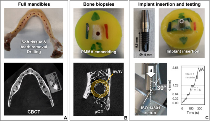
Experimental sample preparation and mechanical testing workflow adapted from a previous study [14]. The soft tissues and teeth of the cadaveric mandibles were removed, a first drilling step was performed, and each mandible was scanned together with a calibration phantom by CBCT for this study (A). The mandibles were cut into individual bone biopsies that were embedded in PMMA and scanned with μCT (B). The monobloc dental implants were inserted in the bone and tested mechanically under cyclic bending‐compression loading (C).

The drilled mandibles were scanned with CBCT (3D Accuitomo 170, J. Morita, Japan). A custom density phantom was placed next to the bones during scanning (Figure 1A). The phantom was made of three commercially available hydroxyapatite‐loaded polymer rods (QRM GmbH, Germany) of known density values (100, 400 and 800 mg/cm³). The image acquisition parameters are reported in Table 1.

TABLE 1.

Scanning parameters used for CBCT and μCT imaging.

	CBCT	μCT
Input voltage	85 kV	70 kV
Current	5 mA	114 μA
Filter	N/A	0.5 mm Al
Exposure time	30.8 s	300 ms
Voxel size	250.0 μm	25.6 μm

Bone biopsies centered on the pilot holes were extracted from the mandibles with a diamond band saw (EXAKT 300, EXAKT Advanced Technologies GmbH, Germany). Following embedding in PMMA cylinders, the specimens were scanned by μCT (μCT 100, Scanco Medical AG, Switzerland) (Figure 1B, Table 1). Prior to implant insertion, an additional drilling step was carried out (Ø3.5 mm). Then, a Ø4.0 mm dental implant with a hybrid monobloc design and adapted extraosseous part (Thommen ELEMENT, Thommen AG, Switzerland) was inserted in the pilot hole of each biopsy. This step was performed free‐handed by an experienced surgeon, and according to manufacturer instructions (Figure 1C). Finally, a custom mechanical testing protocol based on the ISO 14801 standard was applied on the bone‐implant constructs inclined at 30° relative to the vertical axis, either along the oral or vestibular direction (Figure 1C) [11]. A servo‐hydraulic testing machine (858 Mini Bionix, MTS Systems Corporation, USA) was used to apply a low‐cycle bending‐compression loading protocol with sequentially increasing peak displacement at a rate of 1 mm/min. The maximum displacement was doubled every 3 cycles, and the construct was unloaded until reaching 0 N for every cycle (Figure 1C).

2.2. Image Processing

The CT images were processed and used to quantify the peri‐implant bone density to obtain an image‐based primary stability metric [11]. The μCT images of the biopsies were rotated to align the pilot hole axis vertically and segmented using a global threshold determined with Otsu's method. The peri‐implant BV/TV was computed in a region of interest (ROI) is defined as a 1 mm thick hollow cylinder centered on the implant with an inner diameter of 4 mm and a length matching the implant's root. These steps were performed using a custom script implemented in Python 3.8. The CBCT images of the jaw bones were spatially co‐registered with the segmented μCT images of each bone biopsy using Amira (Amira 3D 21.2, Thermo Fischer Scientific, USA). The transformed CBCT image was then resampled at a 100 μm isotropic voxel size in Amira to prevent a loss of information. A linear correspondence between BMD and CBCT GV was established with the density phantom of each scan. The CBCT gray values were converted to BMD units using this relationship. The peri‐implant average BMD was then computed in the same hollow cylindrical ROIs as the μCT‐based BV/TV using the custom Python script.

2.3. hFE Modeling

The hFE modeling workflow previously established for the μCT‐based models to replicate the experiments [14] was applied here to create CBCT‐based models. A simplified axisymmetric implant design, including threads, was modeled as a rigid body. The bone part was generated by subtracting the implant shape from a Ø7.5 mm cylinder with one flat side to indicate the loading direction. Due to the irregular bone surface from site to site, the bone part was extended 5 mm above the implant collar level. The bone part was meshed with linear hexahedral elements, with an edge length set to 0.3 mm at the bone‐implant interface and to 0.7 mm at the external surface, based on a previous mesh convergence study [13]. A contact with a friction coefficient of 0.3 was applied at the bone‐implant interface. The peripheral surface of the bone below the implant collar level was fully constrained. A cyclic vertical displacement was applied to the top of the implant through a reference point located 9.2 mm above the implant collar level to match the experimental setup (Figure 2). The loading protocol mimicked the experimental settings, except that unloading was performed to 0 mm displacement instead of 0 N load.

FIGURE 2.

hFE model geometry and boundary conditions, with the bone peripheral surface being fully constrained (purple), the bone‐implant interface defined as a contact with friction (orange), and a vertical displacement (red) applied to a reference point that drives the rigid body motion of the implant (blue). A cut‐view of the bone part is displayed to show its internal mesh.

The mechanical properties of bone were modeled with an elasto‐plastic constitutive law including damage at large strain [21] and previously established material parameters [14]. In this model, the elastic modulus and the yield stress depend on BV/TV. CBCT‐based BV/TV was deduced from the BMD values by considering that poreless bone (BV/TV = 1) possesses a density of 1200 mg/cm³ [22]. The CT images were spatially registered to the FE mesh, and homogenized properties were attributed to each bone element by averaging the BV/TV of the voxels located inside a Ø1.25 mm sphere centered on its center of gravity (Figure 3). The hFE simulations were run with Abaqus/Standard 2021 (Simulia, Dassault Systèmes, France).

FIGURE 3.

Material mapping procedure for both imaging modalities: the CT images (left) were registered with the hexahedral FE mesh. The BV/TV was computed for each element by averaging the surrounding voxel values. The superpositions of the CT images and the FE mesh mapped with BV/TV are represented, as well as a 3D view of the mapped BV/TV (right).

2.4. Data Evaluation

The experimental ultimate load ($F_{\mathrm{ult}}^{\exp }$) was extracted from the load–displacement curve of each sample. The hFE results were processed in a similar way to obtain a simulated ultimate load, respectively $F_{\mathrm{ult}}^{\mathrm{\mu CT}}$ and $F_{\mathrm{ult}}^{\text{CBCT}}$ for the μCT‐ and CBCT‐based hFE models. Linear regression analyses were performed to compare the primary stability indicators (bone density, experimental and simulated ultimate load). The metrics derived from CBCT images (${\mathrm{BMD}}_{\text{CBCT}}$, $F_{\mathrm{ult}}^{\text{CBCT}}$) were first compared to the ones obtained from μCT images ($\mathrm{BV}/{\mathrm{TV}}_{\mathrm{\mu CT}}$, $F_{\mathrm{ult}}^{\mathrm{\mu CT}}$). Then, all these metrics were correlated to $F_{\mathrm{ult}}^{\exp }$ to assess their ability to predict primary stability. The strength of these correlations was evaluated with Pearson's correlation coefficient (R ²) and interpreted as follows: excellent (R ² > 0.8), good (0.5 < R ² ≤ 0.8), acceptable (0.25 < R ² ≤ 0.5) and poor (R ² < 0.25) [23]. The normalized root mean square error (NRMSE) was evaluated for each variable.

3. Results

The CBCT‐ and μCT‐based results correlated very strongly (R ² > 0.9) for both the bone density based measures (Figure 4A) and the hFE simulations (Figure 4B). However, the converted bone density was approximately 20% lower and the simulated ultimate load was approximately 40% lower for the CBCT‐based models compared to the μCT‐based ones. The NRMSE between $F_{\mathrm{ult}}^{\mathrm{\mu CT}}$ and $F_{\mathrm{ult}}^{\text{CBCT}}$ (21.4%) was two times larger than the error between $\mathrm{BV}/{\mathrm{TV}}_{\mathrm{\mu CT}}$ and ${\mathrm{BMD}}_{\text{CBCT}}$ (10.8%).

FIGURE 4.

Linear regression plots between CBCT‐based and μCT‐based primary stability metrics: bone density (A) and hFE ultimate load prediction (B). The squared correlation coefficient and the normalized root mean square error are indicated for each correlation.

Among the four imaging‐ and simulation‐based metrics, $F_{\mathrm{ult}}^{\mathrm{\mu CT}}$ provided the strongest correlation with $F_{\mathrm{ult}}^{\exp }$ (R ² = 0.81) (Figure 5D). The weakest correlation was obtained with ${\mathrm{BMD}}_{\text{CBCT}}$ (Figure 5A). $F_{\mathrm{ult}}^{\text{CBCT}}$ was a better predictor of $F_{\mathrm{ult}}^{\exp }$ than $\mathrm{BV}/{\mathrm{TV}}_{\mathrm{\mu CT}}$ (Figure 5B,C). For both types of metrics (imaging and hFE), the μCT‐based metrics correlated better with the experimental results than the CBCT‐based ones.

FIGURE 5.

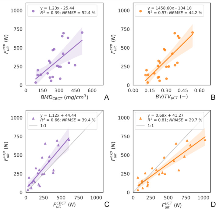
Linear regression plots between the CBCT‐based and μCT‐based primary stability predictor metrics and the experimental ultimate load. The image‐based (A, B) and hFE‐based (C, D) parameters are shown for the image source CBCT (A, C) and μCT (B, D). The squared correlation coefficient (R ²) and the normalized root mean square error (NRMSE) are indicated for each correlation.

4. Discussion

In this study, an hFE model based on CBCT images was developed to predict the primary stability of bone‐dental implant constructs in human jawbones as the key prerequisite for osseointegration and the success of implant therapy. The model's predictions were validated against a previous experimental dataset and compared to μCT‐based hFE models. A few previous studies used CBCT to obtain bone geometry for microFE models [17] or the bone density of a human mandibles [18] for hFE simulations. However, these previous models were not validated with experimental data, and thus the prediction accuracy of simulations utilizing clinically applicable imaging has remained unclear. The encouraging findings of the present study, therefore, provide an important step towards the clinical translatability of the FE simulations.

In the current clinical practice, insertion torque and RFA are commonly used to assess primary stability during implant surgery. While insertion torque can only be measured once during implant placement, RFA can be applied both during surgery and throughout the osseointegration phase during healing. Voumard et al. showed that they correlate well with $F_{\mathrm{ult}}$ experimentally (R ² = 0.94 for insertion torque and R ² = 0.74 for RFA) [11]. The pre‐operative load‐bearing capacity estimator provided by hFE simulations could serve as a valuable complement to intra‐ and post‐operative assessments. Additionally, multiple simulations can be performed to evaluate various implant designs, optimizing primary stability for the specific site. This numerical tool only requires clinically relevant CBCT images and the implant design as an input. It is common to perform a CBCT scans prior to an implant placement surgery, therefore no additional intervention on the patient would be required to apply this tool in a clinical context. Moreover, hFE simulates an occlusal loading mode that can be viewed as more physiologically relevant than the insertion torque and RFA.

The peri‐implant bone density could also be considered as an alternative pre‐operative primary stability estimator given that both ${\mathrm{BMD}}_{\text{CBCT}}$ and $\mathrm{BV}/{\mathrm{TV}}_{\mathrm{\mu CT}}$ correlated significantly with the ex vivo ultimate load. However, the clinically relevant CBCT‐based metric provided the weakest correlation (R ² = 0.39) and largest error (RMSE = 52.4%) among all measures (Figure 5A), which could limit its use in a clinical setting. Although it is more straightforward to obtain such an image‐based metric than performing a simulation, hFE‐based estimators were demonstrated here to be better predictors of the experiment for both imaging modalities (Figure 5). Notably, hFE simulations brought added value to the CBCT images as they estimate $F_{\mathrm{ult}}^{\exp }$ (R ² = 0.66) substantially better than ${\mathrm{BMD}}_{\text{CBCT}}$ (R ² = 0.39).

The reason for the better predictions achieved using the hFE models compared to density‐based measures is that these models include not only the amount of bone but also its spatial distribution and material properties, the implant geometry as well as the load magnitude and direction. The simulated maximum load possesses the same physical meaning as an occlusal load, which can be easier to interpret compared to bone density. However, the simulated force may not represent a physiological scenario. The 30° load inclination used here is adapted from the ISO 14801 standard and is higher than physiological load angles reported in the literature, ranging typically between 10° and 15° for incisors [24]. The resulting high bending moment exerted on the implant makes this loading case a worst‐case scenario. From an engineering perspective, modeling an extreme case provides a safety margin for normal use and represents a conservative approach. Yet the hFE simulations loaded the construct along a single direction (oral or vestibular) to match the experiments. Given that the bone density distribution is not axisymmetric, simulating multiple loading directions (e.g., mesial or distal) would result in different primary stability estimations. This would improve the characterization of the implantation site, notably by determining its weakest loading direction.

In the present study, the previously validated μCT‐based hFE model was taken as a reference point for the CBCT‐based hFE model that was developed here. The meshes, loading and boundary conditions of both models were identical, and the CBCT images were registered to the μCT images to obtain the same position. Therefore, the differences observed between $F_{\mathrm{ult}}^{\text{CBCT}}$ and $F_{\mathrm{ult}}^{\mathrm{\mu CT}}$ can be attributed solely to the different imaging modalities. The results of the two models correlated strongly with each other (R ² = 0.91), but $F_{\mathrm{ult}}^{\text{CBCT}}$ tended to be approximately 40% lower than $F_{\mathrm{ult}}^{\mathrm{\mu CT}}$ (Figure 4B). This discrepancy was probably caused by the lower CBCT‐based BV/TV values that were assigned to the mesh during material mapping (Figure 3), resulting in a weaker simulated bone domain compared to the corresponding μCT‐based counterparts.

Despite the strong correlations between these primary stability estimators, they did not predict the experimental results similarly: the prediction accuracy of the CBCT‐based estimators (${\mathrm{BMD}}_{\text{CBCT}}$ and $F_{\mathrm{ult}}^{\text{CBCT}}$) was consistently lower than for their μCT‐based counterparts ($\mathrm{BV}/{\mathrm{TV}}_{\mathrm{\mu CT}}$ and $F_{\mathrm{ult}}^{\mathrm{\mu CT}}$) (Figure 5). This loss of information observed in CBCT images can be attributed to a number of their characteristics, notably a lower resolution, higher noise and lower contrast than conventional CT [25]. Artifacts such as scattered radiations and beam hardening can also affect the accuracy of the image [26]. In the case of the hFE simulations, some of these effects could be alleviated through the homogenization performed during element material mapping (Figure 3). Nevertheless, the prediction error of $F_{\mathrm{ult}}^{\text{CBCT}}$ (NRMSE = 39.4%) was higher than that of $F_{\mathrm{ult}}^{\mathrm{\mu CT}}$ (NMRSE = 29.7%). This indicates that the relatively small replication error between CBCT‐ and μCT‐based estimators was propagated and even magnified to the prediction error between CBCT‐based estimators and the ex vivo results.

Unlike the μCT images that accurately capture the bone microstructure and can directly assess BV/TV, the two‐steps calibration of the CBCT images relied on simplifications that may have contributed to the prediction error. The density phantom was used here as there are no standardized methods to convert the GV of a CBCT image to BMD [25]. The relationship between the CBCT GV and the density phantom's BMD values was assumed to be linear and this seemed to be reasonable considering the strong correlation between the calibrated ${\mathrm{BMD}}_{\text{CBCT}}$ and $\mathrm{BV}/{\mathrm{TV}}_{\mathrm{\mu CT}}$ in the peri‐implant ROI (Figure 4A). This result is consistent with the findings of some studies, such as that by Cassetta et al. that showed a strong correlation between CBCT GV and clinical CT Hounsfield units (HU) [27]. Yet other papers, including that by Suttapreyasri et al. reported no statistically significant correlation [28]. This lack of consensus has led to the development of new methods to improve the ability of CBCT to capture bone density either in the image acquisition or during post‐processing. For example, Hu et al. employed a multisource CBCT machine, while Park et al. applied a deep learning algorithm to correct the GV in CBCT images [29, 30].

In the hFE model, the bone material properties were defined based on BV/TV, which required an additional calibration step for CBCT. A straightforward approach was used by assuming that poreless bone (BV/TV = 1) had a BMD of 1200 mg/cm³, based on previous reports [22]. The advantage of this approach was that the calibration did not rely on the μCT images. Nonetheless, extrapolating the relationship established between ${\mathrm{BMD}}_{\text{CBCT}}$ and $\mathrm{BV}/{\mathrm{TV}}_{\mathrm{\mu CT}}$ based on the spatially co‐registered images of all samples provided 1.0 BV/TV = 1010 mg/cm³. This mismatch may be attributed to the CBCT imaging, as a stronger beam hardening was reported for denser materials and could induce an underestimation of the cortical bone density [27]. Moreover, the relationship between BMD and BV/TV was assumed to be the same for cortical and trabecular bone. Future studies should investigate if this assumption holds and how this would affect the predicted mechanical behavior.

Despite the lack of a clear consensus concerning the ability of CBCT to quantify bone density, our work showed that a CBCT‐based hFE model could predict the primary stability of dental implants reasonably well: while being less accurate than μCT‐based hFE, it is a better estimator than μCT‐based BV/TV. It should be emphasized that its validation range is limited to one specific configuration. A single CBCT machine type was used with a specific set of acquisition parameters. Besides that, the bones were scanned in the same position. Additional positions of the bone inside the FOV should be investigated as Parsa et al. showed that object positioning and FOV size had a significant impact on the object's GV for CBCT [31]. Unlike conventional CT modalities (e.g., μCT and clinical CT) that possess a fan‐shaped beam, the cone‐shaped beam induces artifacts in the periphery of the FOV, where the beam is not perpendicular to the rotation axis [32]. Furthermore, the reconstruction algorithms can vary from one manufacturer to another; hence, the HU values provided after reconstruction should be interpreted with caution [16]. Direct calibration from GV to BMD based on a density phantom partially overcomes this problem, although the phantom should not be placed too far away from the object of interest. An important limitation of the present study is that the mandibles were scanned isolated and without soft tissues, which is not directly representative of a clinical case. Moreover, the specimens were taken from three male donors, and the results may not represent a larger and more diverse population.

Further limitations of this study are linked to the applied hFE methodology. First, the exact position of the implant was unknown as no post‐implantation imaging was performed. This induced a potential error in the results, but it can be argued that solely using pre‐operative information mimics a prognostic clinical scenario. Further, the modeled implant geometry was simplified, and the impact of small features on primary stability was ignored. At last, each simulation required a computational time of approximately 1000 s to run. By improving the model's computational efficiency, a quick stability estimation could be achieved. The FE‐related limitations have been further elaborated in the previous μCT‐based hFE validation study [14].

Although the present study represents a step forward towards the use of numerical simulations in implantology, several challenges still need to be addressed before its translation to clinical practice, mainly improving the reliability of CBCT images for measuring bone density. Once these challenges are overcome, these numerical models could provide a pre‐operative implant stability metric, allowing clinicians to evaluate different implant positions and dimensions during surgical planning. Another potential application is the longitudinal monitoring of implant stability. The main challenge here is the presence of metal artifacts that can impact the peri‐implant bone GV [26]. Hence, a specific metal artifact reduction algorithm should be developed. Such longitudinal hFE models would also need to be validated with an in vivo study, for instance with RFA.

This study demonstrated that hFE models based on CBCT images could predict the load‐bearing capacity of the bone‐implant constructs in the human jaw with higher accuracy compared to density‐based measures from either CBCT or μCT images. The superiority of the hFE results underlies the strength of this biomechanics‐based approach over density‐based metrics even if using an inferior input image quality. These findings support the translatability of these simulations towards clinical application. The primary stability estimator could become a valuable tool for personalized dental medicine, supporting clinicians in the selection and planning of the optimal implant size and design tailored to the patient's needs. However, there are several challenges to be overcome towards this aim, with an important one being the quantitative calibration of CBCT images into bone mineral density. In the future, such models could be incorporated within a planning software to provide the clinician with a preoperative estimate of primary stability.

Author Contributions

A.V. and P.W. developed the numerical methods and conducted the simulations. R.T. and S.K. performed the experiments. A.V. and R.T. analyzed the data. A.V. and P.V. led the writing. V.C., P.V., and P.Z. supervised the project. P.V. acquired the funding. All authors contributed to the conceptualization of the study, the review, and editing of the manuscript.

Ethics Statement

The human jaws were obtained from donors to the Institute of Anatomy of the University of Bern with informed consent.

Conflicts of Interest

The authors declare no conflicts of interest.

Data Availability Statement

The data that has been used is confidential.

References

- 1. Alghamdi H. S. and Jansen J. A., “The Development and Future of Dental Implants,” Dental Materials Journal 39, no. 2 (2020): 167–172, 10.4012/dmj.2019-140. [DOI] [PubMed] [Google Scholar]
- 2. Bornstein M., Halbritter S., Harnisch H., Weber H., and Buser D., “A Retrospective Analysis of Patients Referred for Implant Placement to a Specialty Clinic: Indications, Surgical Procedures, and Early Failures,” International Journal of Oral & Maxillofacial Implants 23, no. 6 (2008): 1109–1116. [PubMed] [Google Scholar]
- 3. Chappuis V., Rahman L., Buser R., Janner S. F. M., Belser U. C., and Buser D., “Effectiveness of Contour Augmentation With Guided Bone Regeneration: 10‐Year Results,” Journal of Dental Research 97, no. 3 (2018): 266–274, 10.1177/0022034517737755. [DOI] [PubMed] [Google Scholar]
- 4. Haiat G., Wang H. L., and Brunski J., “Effects of Biomechanical Properties of the Bone‐Implant Interface on Dental Implant Stability: From In Silico Approaches to the Patient's Mouth,” Annual Review of Biomedical Engineering 16 (2014): 187–213, 10.1146/annurev-bioeng-071813-104854. [DOI] [PubMed] [Google Scholar]
- 5. Barikani H., Rashtak S., Akbari S., Badri S., Daneshparvar N., and Rokn A., “The Effect of Implant Length and Diameter on the Primary Stability in Different Bone Types,” Journal of Dentistry (Tehran, Iran) 10, no. 5 (2013): 449–455. [PMC free article] [PubMed] [Google Scholar]
- 6. Ruffoni D., Muller R., and van Lenthe G. H., “Mechanisms of Reduced Implant Stability in Osteoporotic Bone,” Biomechanics and Modeling in Mechanobiology 11, no. 3–4 (2012): 313–323, 10.1007/s10237-011-0312-4. [DOI] [PubMed] [Google Scholar]
- 7. Chan H. L., Misch K., and Wang H. L., “Dental Imaging in Implant Treatment Planning,” Implant Dentistry 19, no. 4 (2010): 288–298, 10.1097/ID.0b013e3181e59ebd. [DOI] [PubMed] [Google Scholar]
- 8. Degidi M., Daprile G., and Piattelli A., “Primary Stability Determination by Means of Insertion Torque and RFA in a Sample of 4,135 Implants,” Clinical Implant Dentistry and Related Research 14, no. 4 (2012): 501–507, 10.1111/j.1708-8208.2010.00302.x. [DOI] [PubMed] [Google Scholar]
- 9. Lisiak‐Myszke M., Marciniak D., Bielinski M., Sobczak H., Garbacewicz L., and Drogoszewska B., “Application of Finite Element Analysis in Oral and Maxillofacial Surgery‐A Literature Review,” Materials 13, no. 14 (2020): 3063, 10.3390/ma13143063. [DOI] [PMC free article] [PubMed] [Google Scholar]
- 10. Kim D. G., Jeong Y. H., Chien H. H., Agnew A. M., Lee J. W., and Wen H. B., “Immediate Mechanical Stability of Threaded and Porous Implant Systems,” Clinical Biomechanics (Bristol, Avon) 48 (2017): 110–117, 10.1016/j.clinbiomech.2017.08.001. [DOI] [PubMed] [Google Scholar]
- 11. Voumard B., Maquer G., Heuberger P., Zysset P. K., and Wolfram U., “Peroperative Estimation of Bone Quality and Primary Dental Implant Stability,” Journal of the Mechanical Behavior of Biomedical Materials 92 (2019): 24–32, 10.1016/j.jmbbm.2018.12.035. [DOI] [PubMed] [Google Scholar]
- 12. Chakraborty A., Datta P., Majumder S., Mondal S. C., and Roychowdhury A., “Finite Element and Experimental Analysis to Select Patient's Bone Condition Specific Porous Dental Implant, Fabricated Using Additive Manufacturing,” Computers in Biology and Medicine 124 (2020): 103839, 10.1016/j.compbiomed.2020.103839. [DOI] [PubMed] [Google Scholar]
- 13. Ovesy M., Voumard B., and Zysset P., “A Nonlinear Homogenized Finite Element Analysis of the Primary Stability of the Bone‐Implant Interface,” Biomechanics and Modeling in Mechanobiology 17, no. 5 (2018): 1471–1480, 10.1007/s10237-018-1038-3. [DOI] [PubMed] [Google Scholar]
- 14. Vautrin A., Thierrin R., Wili P., et al., “Homogenized Finite Element Simulations Can Predict the Primary Stability of Dental Implants in Human Jawbone,” Journal of the Mechanical Behavior of Biomedical Materials 158 (2024): 106688, 10.1016/j.jmbbm.2024.106688. [DOI] [PubMed] [Google Scholar]
- 15. Yeung A. W. K., Tanaka R., Jacobs R., and Bornstein M. M., “Awareness and Practice of 2D and 3D Diagnostic Imaging Among Dentists in Hong Kong,” British Dental Journal 228, no. 9 (2020): 701–709, 10.1038/s41415-020-1451-8. [DOI] [PubMed] [Google Scholar]
- 16. Pauwels R., Jacobs R., Singer S. R., and Mupparapu M., “CBCT‐Based Bone Quality Assessment: Are Hounsfield Units Applicable?,” Dento Maxillo Facial Radiology 44, no. 1 (2015): 20140238, 10.1259/dmfr.20140238. [DOI] [PMC free article] [PubMed] [Google Scholar]
- 17. Klintstrom E., Klintstrom B., Pahr D., Brismar T. B., Smedby O., and Moreno R., “Direct Estimation of Human Trabecular Bone Stiffness Using Cone Beam Computed Tomography,” Oral Surgery, Oral Medicine, Oral Pathology, Oral Radiology 126, no. 1 (2018): 72–82, 10.1016/j.oooo.2018.03.014. [DOI] [PubMed] [Google Scholar]
- 18. Bujtár P., Sándor G. K. B., Bojtos A., Szűcs A., and Barabás J., “Finite Element Analysis of the Human Mandible at 3 Different Stages of Life,” Oral Surgery, Oral Medicine, Oral Pathology, Oral Radiology, and Endodontology 110, no. 3 (2010): 301–309, 10.1016/j.tripleo.2010.01.025. [DOI] [PubMed] [Google Scholar]
- 19. Sheikhi M., Karami M., Abbasi S., Moaddabi A., and Soltani P., “Applicability of Cone Beam Computed Tomography Gray Values for Estimation of Primary Stability of Dental Implants,” Brazilian Dental Science 24, no. 1 (2020): 1–8, 10.14295/bds.2021.v24i1.2068. [DOI] [Google Scholar]
- 20. Yingying Z., Zhihong Z., Honghong L., et al., “The Relationship Between Bone Density at Implant Sites and Primary Implant Stability,” International Journal of Dentistry and Oral Health 7, no. 5 (2021): 1–6, 10.16966/2378-7090.370. [DOI] [Google Scholar]
- 21. Schwiedrzik J. J., Wolfram U., and Zysset P. K., “A Generalized Anisotropic Quadric Yield Criterion and Its Application to Bone Tissue at Multiple Length Scales,” Biomechanics and Modeling in Mechanobiology 12, no. 6 (2013): 1155–1168, 10.1007/s10237-013-0472-5. [DOI] [PubMed] [Google Scholar]
- 22. Tassani S., Ohman C., Baruffaldi F., Baleani M., and Viceconti M., “Volume to Density Relation in Adult Human Bone Tissue,” Journal of Biomechanics 44, no. 1 (2011): 103–108, 10.1016/j.jbiomech.2010.08.032. [DOI] [PubMed] [Google Scholar]
- 23. Mukaka M. M., “Statistics Corner: A Guide to Appropriate Use of Correlation Coefficient in Medical Research,” Malawi Medical Journal 24, no. 3 (2012): 69–71, https://www.ncbi.nlm.nih.gov/pubmed/23638278. [PMC free article] [PubMed] [Google Scholar]
- 24. Osborn J. W. and Mao J., “A Thin Bite‐Force Transducer With Three‐Dimensional Capabilities Reveals a Consistent Change in Bite‐Force Direction During Human Jaw‐Muscle Endurance Tests,” Archives of Oral Biology 38, no. 2 (1993): 139–144, 10.1016/0003-9969(93)90198-u. [DOI] [PubMed] [Google Scholar]
- 25. Kim D. G., “Can Dental Cone Beam Computed Tomography Assess Bone Mineral Density?,” Journal of Bone Metabolism 21, no. 2 (2014): 117–126, 10.11005/jbm.2014.21.2.117. [DOI] [PMC free article] [PubMed] [Google Scholar]
- 26. Kaasalainen T., Ekholm M., Siiskonen T., and Kortesniemi M., “Dental Cone Beam CT: An Updated Review,” Physica Medica 88 (2021): 193–217, 10.1016/j.ejmp.2021.07.007. [DOI] [PubMed] [Google Scholar]
- 27. Cassetta M., Stefanelli L. V., Pacifici A., Pacifici L., and Barbato E., “How Accurate Is CBCT in Measuring Bone Density? A Comparative CBCT‐CT In Vitro Study,” Clinical Implant Dentistry and Related Research 16, no. 4 (2014): 471–478, 10.1111/cid.12027. [DOI] [PubMed] [Google Scholar]
- 28. Suttapreyasri S., Suapear P., and Leepong N., “The Accuracy of Cone‐Beam Computed Tomography for Evaluating Bone Density and Cortical Bone Thickness at the Implant Site: Micro‐Computed Tomography and Histologic Analysis,” Journal of Craniofacial Surgery 29, no. 8 (2018): 2026–2031, 10.1097/SCS.0000000000004672. [DOI] [PubMed] [Google Scholar]
- 29. Hu Y., Xu S., Li B., et al., “Improving the Accuracy of Bone Mineral Density Using a Multisource CBCT,” Scientific Reports 14, no. 1 (2024): 3887, 10.1038/s41598-024-54529-4. [DOI] [PMC free article] [PubMed] [Google Scholar]
- 30. Park C.‐S., Kang S.‐R., Kim J.‐E., et al., “Validation of Bone Mineral Density Measurement Using Quantitative CBCT Image Based on Deep Learning,” Scientific Reports 13, no. 1 (2023): 11921, 10.1038/s41598-023-38943-8. [DOI] [PMC free article] [PubMed] [Google Scholar]
- 31. Parsa A., Ibrahim N., Hassan B., van der Stelt P., and Wismeijer D., “Influence of Object Location in Cone Beam Computed Tomography (NewTom 5G and 3D Accuitomo 170) on Gray Value Measurements at an Implant Site,” Oral Radiology 30 (2014): 153–159, 10.1007/s11282-013-0157-x. [DOI] [Google Scholar]
- 32. Molteni R., “Prospects and Challenges of Rendering Tissue Density in Hounsfield Units for Cone Beam Computed Tomography,” Oral Surgery, Oral Medicine, Oral Pathology, Oral Radiology 116, no. 1 (2013): 105–119, 10.1016/j.oooo.2013.04.013. [DOI] [PubMed] [Google Scholar]
Associated Data
This section collects any data citations, data availability statements, or supplementary materials included in this article.