FPGA implementation of a complete digital spiking silicon neuron for circuit design and network approach

Abstract

When attempting to replicate the same biological spiking neuron model actions of the human brain, the spiking neuron model methodology and hardware realization design for the nervous system of the brain are crucial considerations. This work provides a modified neural modeling of complete Digital Spiking Silicon neuron model (DSSN4D). This model is capable for regenerating the basic attributes of the original model using a simplified power-2 based modeling technique. The suggested spiking neuron model is based on the fundamental power-2 based operations that can be implemented similar to the basic attributes of the main model. Removing the nonlinear parts of the main model (original one) and replacing them with modified ones leads to achieving a low-cost, low-error, and high-frequency digital system rather than the original modeling. A Xilinx Virtex-7 XC7VX690T FPGA board has been thought of and utilized for hardware realization and of the proposed model (this can validate the proposed system). The original and proposed models (in terms of neural activities) exhibit a significant degree of resemblance, according to hardware results. Additionally, greater frequency and low-cost conditions have been attained. Results of implementation indicate that overall savings are higher than for other papers and the original approach. Additionally, the new neural model’s frequency, which is roughly 502.184 MHz, is much greater than the original model’s frequency, which was 224 MHz. Also, results in hardware level shows that the proposed model takes a maximum 0.01% of the available resources of a Virtex-7 FPGA board.

Introduction

Spiking neural networks (SNNs) are a fascinating area of study that combines Artificial Intelligence (AI) with Neuromorphic Engineering (NE). This discipline has real-world applications in areas like memory, learning, medicine, data processing, etc^1–6.

The human brain is divided into several sections, and each section is made up of fundamental components: spiking neuron model cells connected by synapses. In the study of neural systems, it is crucial to recognize the diversity of neuron types that exist. Each type of neuron plays a unique role in neural circuitry, contributing to different functions such as sensory processing, motor control, and cognitive functions. For instance, excitatory neurons, such as pyramidal cells, facilitate signal transmission, while inhibitory neurons, such as interneurons, regulate and balance excitatory activity, ensuring overall network stability. Understanding the interactions between these various neuron types can provide insights into the complex dynamics of neural systems. Ordinary Differential Equations (ODEs) are typically used in mathematical applications to represent the functioning of spiking neuron models. To mimic genuine spiking neuron models, a variety of models at various biological levels have been published^7–13. They are computationally expensive since they are based on biologically specific spiking neuron model models. As a result, the amount of biological complexity and computing expense must be balanced when selecting a suitable model for the simulation and implementation of spiking neural networks. In our paper, the Complete Digital Spiking Silicon spiking neuron model (DSSN4D) model is applied for hardware implementation process⁷. The goal of this model was to imitate several kinds of spiking neuron models using straightforward digital arithmetic circuits.

In case of hardware implementation, there are two basic approaches that can be considered: Analog and Digital. The analog case has several advantages over digital ones, such as being easier to communicate with real-world signals and using less power and area. On the other hand, this technique has several drawbacks such being difficult to use, susceptible to process variability, and noise. Every change in its parameters results in a modification in the design. Different papers in this field have been presented in case of analog realization of models^14–18. On the other hand, high power consumption, a large silicon need, and discretization over time are drawbacks of digital system architecture. Moreover, they have simple, multiple spiking neuron model simulations, flexibility in design, and are noise-resistant (and process variability). Recently, a reconfigurable system using an FPGA presented a high resource case to observe the activity of the spiking neuron models in neural networks as well as dynamical behaviors^19–28.

In this work, a hardware implementation of complete version of DSSN modeling (DSSN4D) for digital systems is proposed. The main challenge in this implementation is the quadratic term of the original spiking neuron model model. In most cases, the quadratic term slows down the final system because of its multiplier action. In other words, the Central Nervous System (CNS) depends greatly on the rate of neural activity. The CNS is comprised of the brain and spinal cord and is responsible for integrating sensory information, processing cognitive functions, and directing motor responses. It plays a critical role in regulating vital bodily functions such as breathing, heart rate, and coordination of movement. CNS is also central to higher cognitive functions, including memory, language, and decision-making. Neurons within the CNS communicate through complex signaling pathways, utilizing neurotransmitters and electrical signaling to relay information. The study of the CNS is essential in understanding various neurological disorders and developing therapeutic strategies.

The neurological system is affected if the final system’s frequency is unacceptable. This nonlinear phrase must thus be eliminated or changed to another simple function. To create basic mathematical equations, many methods might be applied. The best method among them would be to transform the quadratic terms into power-2 based functions. Indeed, while conserving all behaviors of the original model, By converting the nonlinear components of the original model into a set of power-2 terms, we have a new model that converts all multiplier operations into a sequence of digital SHIFTs and ADDs (this method will be explaied). The suggested new model provides a low-cost, quick, and efficient system that can execute and trace the original spiking neuron model model with a high degree of resemblance.

However, compared to original model and also earlier efforts^29,30, the provided DSSN4D model is substantially more accurate and does not have the aforementioned flaws. The investigation shows that the original forms and dynamics can be successfully recreated using our approach. Because all nonlinear components are eliminated when employing base-2 functions, there is a high matching similarity and multiplierless implementation. This results in the creation of a digital system that is quick, inexpensive, and capable of large-scale digital implementation.

Biological neural systems comprise a wide variety of neuron types, each exhibiting distinct electrophysiological behaviors that support cognitive functions, motor control, and sensory processing. These neurons, classified based on their spiking patterns and synaptic connectivity, include regular spiking (RS), fast spiking (FS), intrinsically bursting (IB), low-threshold spiking (LTS), and chattering (CH) neurons, among others. Simulating and implementing such diversity is a key challenge in neuromorphic engineering and computational neuroscience. While our study primarily focuses on the Digital Spiking Silicon Neuron (DSSN4D) model, this approach is not restricted to a single neuron type. The DSSN4D model is a generalized digital neuron framework that can replicate various neuronal behaviors through parameter tuning and structural adjustments. The core dynamical properties-membrane potential evolution, recovery mechanisms, and spike generation-allow DSSN4D to serve as a flexible template for multiple neuron types. By modifying key model parameters, different firing patterns can be generated, demonstrating its adaptability beyond a single neuron. Additionally, the power-2 based approximation technique introduced in this study is a universal optimization method that can be applied to various neuron models. This method reduces computational complexity while maintaining fidelity to biological neural behaviors, making it suitable for large-scale neuromorphic systems. In this work, we validate the feasibility of DSSN4D by demonstrating its efficiency in digital implementation; however, its potential extension to other neuron types is a natural progression of this research. This study lays the groundwork for scalable hardware-friendly neuron implementations, paving the way for the future realization of heterogeneous neural populations on digital platforms.

The rest of the paper is organized as follows. In Section II, complete DSSN4D spiking neuron model model is briefly presented. In Section III, the proposed approach is explained. Proposed model simulation and validation are described in Section IV. In Section V, a population test is evaluated. The proposed model design and implementation process are presented in Section VI. Finally, FPGA results and conclusion are given in Sections VII and VIII, respectively.

Complete DSSN modeling (DSSN4D)

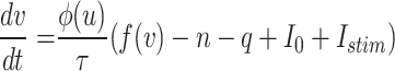
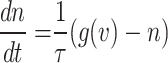
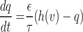
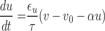
The primary DSSN model⁷ is a spiking neuron model model that uses fixed point operation and Euler’s approach to mimic several kinds of neural processes. A qualitative neural model, the DSSN model was developed to be effectively implemented in digital circuitry. Intrinsically Bursting (IB) class spiking neuron models are a specific type of spiking neuron model characterized by their ability to generate bursts of action potentials (spikes) in response to depolarizing stimuli. This bursting behavior is intrinsic to the spiking neuron model’s properties, often resulting from the interplay of various ion channels, including calcium and sodium channels. IB Class spiking neuron models are crucial for various functions in the CNS, such as rhythmic activities and synchronizing neural networks. Their unique firing patterns contribute to processes like the generation of rhythmic movements and the modulation of sensory input. Thus, The complete version of DSSN modeling called DSSN4D model with four variables that is expressed as follows:

1

2

3

4

Where

5

6

7

8

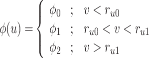
Accordingly, the slow variable and the voltage are represented in these equations by the symbols v and n. On the opposite side, the membrane potential is represented by v, and n is the recovery variable used to create the voltage variable. Additionally, the applied current is and the value is a bias fixed parameter. Table 1 contains the additional inputs for creating the IB class patterns. The slow variable, or q, abstractly denotes the ion channel activity. The value of the new variable u is adjusted dynamically. Since is chosen from the list of potential values and the equation of u does not include multiplication between variables, it does not increase the number of multiplications in a step of numerical integration. The variables’ time constants are controlled by the parameters , , and . In the case when or hp, the parameters and are constants that modify the nullclines of the variables. This qualitative model contains only abstract, non-physical variables and constants.

Table 1.

Fixed parameters for spiking patterns generation in IB class of complete DSSN model (DSSN4D).

Parameter	Value	Parameter	Value	Parameter	Value
	4		− 0.5		2.4
	− 0.3		2.4		0.4
	0.3		3.5		− 10
	20		0.75		− 9.6
	− 0.18		− 1.5		0.2
	1.6		− 1.6		0.17
	0.8		− 1.6		0.002
	0.0008		0.0005		− 7.6
	0.2		0.23		0.35
	0.36		0.38		− 2

IB class spiking neuron models may be achieved using parameter settings by choosing the proper values for these parameters. Finally, as shown in Fig. 1, various spiking patterns depending on these fundamental factors may be simulated. Indeed, this figure demonstrates how varying the applied stimulus currents directly influences the spiking frequency of the DSSN4D model. This relationship highlights the model’s sensitivity to input, which is a fundamental characteristic of spiking neuron behavior. Specifically, as the intensity of the stimulus current increases, the frequency at which the neuron fires action potentials also rises, illustrating the neuron’s ability to encode information through changes in firing rate. This sensitivity to input is not only crucial for understanding the dynamics of individual neurons but also underpins the larger network behaviors that emerge in neural circuits, making it a vital concept in the study of computational neuroscience.

Fig. 1.

Spiking voltage waveforms for the original DSSN4D model in different stimulus.

Proposed approach

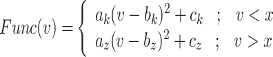
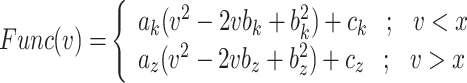
For achieving the best and high-accurate modifying the original model, the nonlinear terms of DSSN4D model must be approximated. The quadratic component, which is repeated throughout the whole model, is its primary nonlinear term, as it is illustrated in the equations of the original DSSN4D model. Although a DSSN4D spiking neuron model is built on an FPGA digital board, the final system is not more efficient due to the quadratic components in the equations. In this case, changing the nonlinear terms into new functions is the best option. To do this, there are two prerequisites: first, the original and proposed methods must be highly similar; second, the digital implementation must be low-cost in terms of FPGA resources and faster than the original DSSN4D model. There are different methods for modifying the nonlinear and high-cost terms of the original model including piecewise linear functions, absolute functions, trigonometric approach, dynamic-reduced, hyperbolic expressions, and power-2 based method. The amount of inaccuracy in the suggested model can rise when linear functions are used to approximate the original models, however utilizing power-2 functions results in lower error calculations and also higher levels of similarity. Thus, we employed the power-2 functions in this research. Another advantage of this method is that by using these hyperbolic terms, all nonlinear variables and functions in differential equations are transformed to digital SHIFTs and ADDs without any multiplications. As a result, we now have a new model that incorporates every component of the original model and is more effective than the original primary DSSN4D model in terms of speed and cost. The equations are rewritten in the suggested model as follows:

9

10

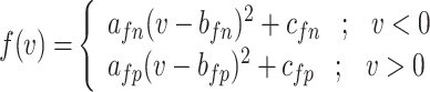
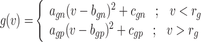
where

11

The inclusion of Eqs. (9) and (10) in this study is pivotal for elucidating the transformation of complex nonlinear dynamics into a more manageable form suitable for hardware implementation. Equation (9) captures the nonlinear characteristics of the original Digital Spiking Silicon Neuron (DSSN4D) model, detailing how these dynamics are defined in relation to the voltage variable v. Transitioning to Eq. (10) demonstrates our approach to approximating these nonlinearities using a power-2 based function G(v), which enables efficient computations through simple digital operations such as shifts and additions. This systematic transition not only enhances computational efficiency but also ensures the fidelity of the model’s dynamic behavior, thereby bridging the gap between theoretical nonlinearity and practical implementation.

Thus, the nonlinear term of the DSSN4D model, (F(v)) is replaced by a power-2 based function (G(v)), with high-accuracy matching and low-error state based on Table 2 index considerations. In this approach, as illustrated in Fig. 2, the basic term () and the proposed power-2 based term (G(v)) are in high similarity cases. For achieving the best parameters of the proposed approach, , we have utilized an exhaustive search algorithm. In this case, an error function is applied as . Three basic parameters of the proposed function, can be selected when this error function is less than the fixed low value, . The iteration of this algorithm is repeated until the best parameters of the proposed function are extracted. Using this method, the optimized parameter values are selected as: , , and .

Table 2.

Basic functions and corresponding index of the proposed approach.

Func(v)	k	x	z
f(v)	fn	0	fp
g(v)	gn		gp
h(v)	hn		hp

Fig. 2.

Approximation of nonlinear term (F(v)) by the power-2 based function (G(v)) with calculated error between two functions.

The power-2 based method offers significant advantages in reducing nonlinearity and enhancing system performance. By transforming traditional nonlinear multiplication operations into simpler arithmetic operations like addition and bit-shifting, this approach not only simplifies computations but also mitigates nonlinearity in signal processing. Importantly, the elimination of resource-intensive multipliers leads to a substantial decrease in latency, which is crucial for real-time processing applications requiring high-frequency operations. This method allows for a remarkable increase in operational speed, with frequencies reaching up to 502.184 MHz, thereby enabling the system to manage more computational tasks within the same timeframe. Additionally, the use of basic arithmetic operations significantly reduces resource consumption on FPGA platforms, resulting in fewer Flip-Flops (FFs) and Look-Up Tables (LUTs) compared to the original model, thus improving overall design efficiency. The resulting hardware simplicity not only promotes cost-effectiveness but also supports scalability for larger networks of spiking neuron models, optimizing resource utilization.

Simulation results and model validation

For the suggested model to be validated, two fundamental elements must be taken into account. In this method, it is crucial that the suggested model be in the same state as the original model in terms of phase portrait behaviors and it is also crucial that the time domain analysis for the two models-original and proposed-be performed with minimal error.

In case of patterns similarity, the time domain must be taken into account in order to validate the proposed spiking neuron model model in terms of timing precision and spiking patterns. This method compares the spiking patterns of the original and suggested DSSN4D models using various stimulus currents. As seen in Fig. 3, the presented spiking neuron model model’s spiking patterns have a striking resemblance to those of the original model.

Fig. 3.

Patterns comparison for two models (DSSN4D and proposed) by the stimulus currents as: , , , and .

To further study the behaviours of the proposed DSSN4D model, for 4 trigger cases, phase portraits of oscillations are plotted between , , and with in Figs. 4. Considering results of these simulations (timing analysis and phase portrait shapes), proposed model was selected for digital implementation. Simulation results confirm that the new model follows the DSSN4D model in high-degree of similarity and accuracy.

Fig. 4.

Different shapes of the phase portrait for the original DSSN4D and proposed models. All trigger levels have been tested for validating the proposed model in case of phase portraits.

As shown in Fig. 3 and Fig. 4, there are discrepancies (error) between the original and suggested DSSN4D models in various regions of the spiking patterns. In fact, efforts are being made to minimize this mistake to almost nil. There are several methods for calculating the differences between the original and proposed models’ error levels. The formulation of these techniques is as follows:

12

13

14

15

16

In above equations, the variable can be equal to , , , and . Since the discrepancies between our suggested model have been reduced to a minimum, the updated model reproduces the original model’s spike-based behaviors with a high degree of resemblance and low computation error. The computed error levels are displayed in Table 3 for different stimulus currents.

Table 3.

Errors criteria to measure difference between proposed model and original DSSN4D.

Error	v				q				n				u
	I = 0.6	I = 0.7	I = 0.8	I = 1	I = 0.6	I = 0.7	I = 0.8	I = 1	I = 0.6	I = 0.7	I = 0.8	I = 1	I = 0.6	I = 0.7	I = 0.8	I = 1
RMSE	0.12	0.11	0.14	0.2	0.08	0.07	0.1	0.3	0.09	0.05	0.04	0.13	0.14	0.12	0.1	0.06
NRMSE %	1.23	1.11	1	1.2	2.08	3.07	1.1	1.3	1.12	2.12	1.11	1.18	2.02	2.07	1.03	1.33
MAE	0.02	0.01	0.04	0.02	0.08	0.07	0.01	0.03	0.09	0.05	0.04	0.03	0.04	0.02	0.01	0.06
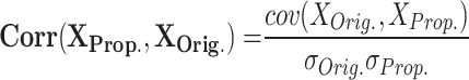
Corr %	96	96.5	95.5	98	99	99	99	99	99	99	99	97	97	96	94	94
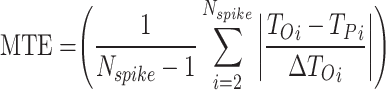
MTE	0.01	0.01	0.01	0.02	0.05	0.03	0.01	0.02	0.06	0.05	0.01	0.04	0.08	0.08	0.01	0.02

RMSE measures the average magnitude of the errors between predicted and observed values, sensitive to large errors; a lower RMSE indicates a better fit. MAE calculates the average absolute difference between predicted and actual values, treating all errors equally and showing less sensitivity to outliers; a smaller MAE denotes a more accurate model. NRMSE is the RMSE divided by the range of the observed data, providing a scale-independent measure for comparison. The correlation coefficient evaluates the strength and direction of the linear relationship between two variables, with values ranging from − 1 to 1; closer to 1 suggests a strong positive correlation, near − 1 indicates a strong negative correlation, and around 0 implies no correlation. MTE assesses the accuracy of spike timings between two models, averaging the differences in spike timings and giving insight into prediction accuracy. To enhance clarity, we define the parameters related to the error metrics introduced in Eqs. (12)–(16) as follows:

• and : These variables represent the data points from the proposed and original models, respectively. They are critical for measuring the differences in neuron behavior between the two models.

• n: This signifies the total number of data points considered for error calculations. It plays a pivotal role in ensuring statistical accuracy in the calculations of Root Mean Square Error (RMSE) and Mean Absolute Error (MAE).

• and : These are the maximum and minimum values observed in the dataset. They are employed in the calculation of Normalized RMSE (NRMSE) to appropriately scale the error between the proposed and original models.

• and : These values represent the standard deviations of the original and proposed model datasets, respectively. They are utilized in the computation of the correlation coefficient to evaluate the degree of correspondence between the two models.

• : This term denotes the covariance between the outputs of the original and proposed models, quantifying the extent to which the two models vary in tandem.

• : This parameter indicates the total number of spikes analyzed when calculating the Mean Timing Error (MTE), providing insight into the timing accuracy of the model.

• and : These values represent the timing of the spike for the original and proposed models, respectively. They are essential for comparing differences in spike timings.

• : This variable signifies the inter-spike interval of the original model, which is used to normalize timing discrepancies in the MTE calculation.

These definitions have been added to the revised manuscript to provide greater clarity in understanding the Eqs. (12)−(16).

Our proposed model has successfully replicated several key attributes of the original Complete Digital Spiking Silicon spiking neuron model (DSSN4D) model. These include precise spiking patterns in response to various stimulus currents, closely matched voltage dynamics, and consistent behaviors of recovery variables, which together validate the temporal and functional accuracy of our approach. However, we also acknowledge areas where our model falls short. Specifically, simplifications of nonlinear dynamics may limit the model’s ability to simulate complex spiking neuron model firing patterns, while extreme excitatory or inhibitory conditions might expose limitations in capturing nuanced behaviors. Furthermore, the original model’s inherent sensitivity to parameter variations is not fully represented in our approach. Thus, while our work demonstrates considerable fidelity to foundational behaviors of the DSSN4D, we remain aware of existing complexities and plan to address these in future research endeavors.

Table 3 presents key error metrics that assess the performance of the proposed modified Complete Digital Spiking Silicon Neuron (DSSN4D) model compared to the original model across various stimulus currents. The metrics include RMSE, NRMSE, MAE, and correlation coefficients, which collectively demonstrate the accuracy and reliability of the proposed model. With RMSE values ranging from 0.11 to 0.20 and NRMSE percentages under 3%, the proposed model consistently exhibits low error margins, signaling a strong alignment with the original model’s spiking patterns. Additionally, the MAE values between 0.01 and 0.09 further emphasize the high fidelity of the proposed model, while correlation coefficients exceeding 94% indicate a robust linear relationship. These findings underscore the significant advancements achieved by the proposed model, validating its potential for applications in neuromorphic computing and highlighting its ability to closely replicate biological neuron dynamics.

Population test

We examined the viability of our presented case by simulating its behavior within a large-scale network comprising a thousand interconnected spiking neuron models. Each of these utilizes modules that connect to others via 100 distinct synapses. The trigger signal for the spiking neuron model cell can be expressed by the following equation:

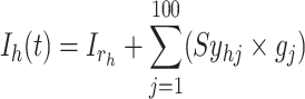17

represents a random input current to the spiking neuron model. The synaptic weight is indicated by . Excitatory synapses are assigned a weight of , while inhibitory synapses receive a weight of . Additionally, has a value of when the spiking neuron model is firing and at all other times. The raster plots for the current and presented cases are displayed in Fig. 5. It is clear that the two models demonstrate a general resemblance. However, they show similar spiking activity. To analyze the variations in network performance between the existing and proposed models, a Mean Relative Error (MRE) criterion is introduced. This can be formulated as:

18

Here, represents the time gap between the spike of our modeling and the basic DSSN4D model, and N denotes the sample count. The computed MRE for various applied currents is below .

Fig. 5.

A simulation of a population of 1000 spiking neuron models with random connections. For the DSSN4D and proposed models, four modes are taken into account by the stimulus currents as: , , , and .

In our analysis, we utilized several metrics, including Root Mean Square Error (RMSE), Mean Absolute Error (MAE), and correlation coefficients, to assess the similarity between the spiking activity of the proposed DSSN4D model and the original model during single spiking neuron model simulations. These metrics provided valuable insights into error magnitude and correlation at the micro-level. However, for population simulations involving 1000 randomly connected spiking neuron models, we shifted our focus to the Mean Relative Error (MRE) as it effectively captures overall accuracy while considering the scale of spiking neuron model interactions. The MRE is particularly suitable for large datasets, as it expresses error in relative terms, offering a clearer understanding of model performance across diverse spiking outputs. By adopting MRE for our population analysis, we ensure that our evaluation reflects both individual spiking neuron model behavior and population-level dynamics, with the MRE of 1.12% indicating that the proposed model maintains high fidelity to the original model’s spiking dynamics, thus reinforcing its validity for simulating complex neural populations.

Design and hardware implementation

The hardware digital circuits and FPGA realization of the proposed model is suggested in this section. To have an optimized and low-cost implementation, all nonlinear terms and variable-parameter multiplications are converted to digital shifters and adders.

Scheduling circuits

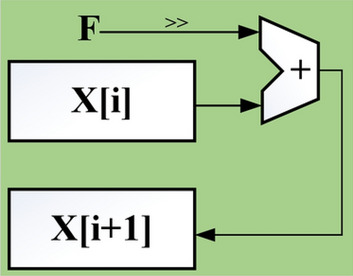
The proposed scheduling diagrams based on the proposed model is depicted in Fig. 6 utilizing just inexpensive building pieces like ADDs, SUBs, and digital SHIFTs without any multipliers. Different parts must be assessed in order to obtain a final digital design, as can be seen in the following subsections. In order to achieve the final fundamental signal, , we employed internal functions using the independent Control Unit (CU). The timing process and scheduling diagrams must be shown in order to have a proper hardware design. This process aids in having an ideal design with the fewest number of resource units and the shortest delay duration, which results in a high-frequency system. All multiplications and divisions are accomplished via digital shifts to the right or left in order to optimize the final hardware in terms of resources cost.

Fig. 6.

Realization of proposed digital diagrams for the proposed model. The internal term, is applied to calculate the basic variables of model.

Equation discretization

Scheduling diagrams must be created using the discretized proposed equations in the case of digital implementation. Although there are other methods for doing this, we have utilized the Euler approach in this instance as below:

19

20

21

The representation of this approach is shown in Fig. 7. Also, in discretized method, is the time step.

Fig. 7.

The Euler method representation using for the proposed model realization.

System bit-width

The final system’s bit-width must be established in order to have an optimum digital implementation. Digital displays often show numbers in fixed-point and floating-point formats. Floating-point displays provide significantly higher levels of precision than fixed-point displays, but they also need more digital resources to construct and slow down the finished circuit. The fixed-point technique is employed in actuality and in the majority of processing systems that are built using FPGA, particularly where speed is crucial and resources are constrained. As a result, the range of every variable in digital design is calculated. The precision of the bits number used to assess the integer and fractional components is typically traded off with the bits number. After all variables and parameters considerations, for avoiding any data removing and protecting the complete calculations, the maximum required shifts to the right or left should be considered to have an efficient system. Consequently, the final digital bit-width of the proposed model is equal to bits. In this procedure, bit is for variable signs, bits for the integer part and bits for the fractional part.

Overall architecture

The recommended architecture of the digital circuit design must be taken into consideration after providing the scheduling diagrams of the proposed model. Figure 8 shows the suggested model’s general design.

Fig. 8.

The proposed architecture design for the final digital system consisting different basic blocks.

Basic values unit (BVU)

This unit provides the basic values of fixed parameters and also initial values of the basic variables. One SRAM and one register are applied to store these values. In this approach, as can be depicted in Fig. 9, the outputs of these two RAMs, are considered for the inputs of a multiplexer module to select the evaluated initial considerations that are used for the spiking neuron model Unit (NU). Moreover, for avoiding any data loss, a is considered in the final outputs of this sub-module.

Fig. 9.

The proposed circuit for implementing the BVU.

Spiking neuron model unit (NU)

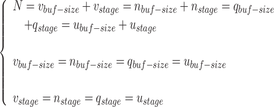
In this part, by applying the pipelining approach, spiking neuron model productions speed will be increased, significantly. For a pipeline implementation of the proposed model, four buffers (, , , and ) are considered. In this figure, , , , and are realized in , , , and stages, respectively. In Fig. 10, , , , and are the storage blocks. The bit-width of every unit of the buffers is the same as in the , , , and modules, which are determined according to the required accuracy. Accordingly, the following conditions must be satisfied:

22

For an appropriate operation of the pipeline structure (satisfying the third equation), synchronization between the , , , and structures is needed.

Fig. 10.

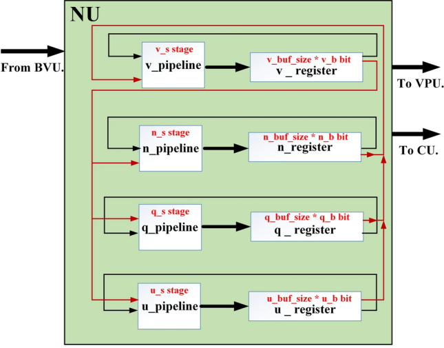
Overall structure for implementing the pipelining design.

Control unit (CU)

In this unit, all internal functions, required signals, and power-2 based term are created for controlling the other parts of system architecture. As it is illustrated in Fig. 11, at firts, the voltage variable values are evaluated for applying to the power-2 based module (based on different parts of the Eq. 11). After that, the basic part of the proposed system (), can be realized based on the Eq. (10). By providing this internal term, the required data can be applied to the spiking neuron model Unit (NU). Moreover, other internal functions are evaluated based on different levels of the voltage signal in this architecture. Additionally, the basic concept in this part is providing the powe-2 based function. In this approach, two parts of voltage signal are seprated based on integer and fraction sections. Then, right and left shifts of signal are added based on positive and negative values of voltage variable. Finally, based on sign-bit, the output can be achieved.

Fig. 11.

Implementing the Contronl Unit (CU) and providing different internal functions and power-2 based term of the proposed system.

Voltage provider unit (VPU)

This unit provides the final voltage signal as can be shown in Fig. 12. In this approach, a is used for storing the final voltage data. After that, an 8-bit selector is applied for final signal selecting. This selected data is applied to an 8-bit DAC for providing the final voltage signal.

Fig. 12.

The circuit for providing the final voltage variable signal.

FPGA results

In case of implementtaion results, verilog hardware description language was used to put the final designs into practice. After validated, created HDL codes were then synthesized by Xilinx ISE XST and downloaded into Virtex-7 XC7VX690T FPGA board. This was done after they had been simulated in Modelsim software. In this instance, the VGA port’s Digital to Analog Converter (DAC) converts the on-FPGA data to analog. Fig. 13 displays oscilloscope shapes of the embedded FPGA. This figure shows the proposed model of an FPGA-implemented model that corresponds to computer simulation findings. With high degrees of matching states, as can be shown in this figure, the hardware spiking patterns resemble the simulation behaviors. Moreover, the hardware patterns mimic the spiking patterns of the original model. In this case, we have applied the for calculating the absolute error levels between proposed model patterns in simulation and implementation conditions as below:

23

Table 4 shows the calculated errors in this case for 4 different states.

Fig. 13.

The digital data for voltage signal in the proposed model in case of different trigger as: (a) and (b) .

Table 4.

MAE For spiking patterns in hardware and simulation cases.

Trigger	MAE
	0.025
	0.033
	0.021
	0.022

Table 5 displays the final reports on the realization of the original and proposed models with regard to hardware resources and implementation. As shown in the table, the resources needed for the suggested model’s implementation are in better state than those needed for the original model and other comparable works in^29,30. In addition, the original model makes use of DSP FPGA units, which lowers the overall frequency and increases the number of implemented spiking neuron models per FPGA core. With larger number of the multipliers, the utilization of FPGA resources is increased in the original model. The presented Table is considered for implementing the number of spiking neuron models (for the proposed model) leads to maximum number of resources used in one FPGA core. Also, a comparison between our proposed model and the implemented DSSN model in³¹ (the basic model of DSSN with two variables) is presented in the mentioned table for complete presentation.

Table 5.

Resource utilization and Speed for FPGA implementation of DSSN4D models (Original DSSN4D, proposed model, and presented DSSN4D in^29,30, and the basic DSSN presented in³¹).

Model	FFs	LUTs	DSPs	Speed (MHz)	IN
Orig. Model (Virtex-7)				224	294
Prop. Model (Virtex-7)			−	502.184	1000
Orig. Model (Spartan-3)				76	1
Prop. Model (Spartan-3)			−	132.5	3
29				NA	334
30				NA	625
31			NA	168	2

The number of implemented spiking neuron models depends on the resources available in a given FPGA core. In fact, the maximum number of FPGA resources may serve as a restriction on this quantity. As a result, the Resource Usage (RS) factor for each resource is displayed as follows:

24

In this case, the Maximum Resource Usage (MRS) is given as:

25

By MRS, the maximum number of spiking neuron models can be calculated on one FPGA core. In this approach, the FPGA Resources can be selected by maximum percentage of the basic resources of FPGA core as: , , , and . The parameter of maximum spiking neuron models number is calculated using Implemented spiking neuron models (IN) as the following equation:

26

These numbers for original, proposed and other similar models are presented in the Table 5. As data indicates, the number of proposed model that could be implemented on FPGA, is higher than that of other similar models. As depicted in this table, in the our proposed model, the speed level (frequency) and also, the overhead-cost are in the better conditions compared with the original DSSN4D model. It is noticeable that the parameter is a basic factor for scaling the number of implemented proposed model on one FPGA core. Consequently, two basic factors, and validate that our proposed model is more efficient than the original model and also other similar works. This Table provides a comprehensive comparison of resource utilization and operational speed for various implementations of the DSSN4D models across two FPGA architectures: Virtex-7 and Spartan-3. The data reveals that the proposed model on the Virtex-7 architecture delivers outstanding performance, achieving a maximum speed of 502.184 MHz while utilizing significantly fewer resources compared to the original model, as indicated by the reduced number of flip-flops (FFs) and lookup tables (LUTs). When examining the Spartan-3 implementation, the proposed model also demonstrates a noteworthy reduction in resource consumption, with only 341 FFs and 511 LUTs needed, as opposed to the original model that required 710 FFs and 1520 LUTs. Despite the lower performance on the Spartan-3 platform, where the speed is limited to 132.5 MHz, the results underline the proposed model’s enhanced efficiency and suitability for environments with resource constraints. This comparative analysis illustrates that while the Virtex-7 implementation excels in speed, the Spartan-3 version provides a compelling option for scenarios where resource utilization is critical, clearly emphasizing the versatility of the proposed model across different FPGA architectures.

Also, Table 6 shows the superiority of our proposed model to the original modeling in case of resources and speed.

Table 6.

Comparison of original and proposed models.

Metric	Original model	Proposed model
Flip-Flops (FFs)	210 FFs	92 FFs (56% reduction)
Look-Up Tables (LUTs)	1510 LUTs	458 LUTs (70% improvement)
Digital Signal Processors (DSPs)	1 DSP slice	0 DSP resources
Peak Frequency	224 MHz	502.184 MHz
Implemented spiking neuron models (IN)	Limited capacity	Up to 1000 spiking neuron models
Resource Usage (FFs)	0.02%	0.01%
Resource Usage (LUTs)	0.34%	0.1%
Qualitative Performance	Standard spiking dynamics	Improved dynamics, more robust

The FPGA resource utilization values presented in Table 5 are obtained from post-synthesis and post-place-and-route (P&R) reports using Xilinx ISE XST on a Virtex-7 XC7VX690T FPGA. These values accurately reflect real hardware constraints, including routing congestion, signal delays, placement overhead, and resource sharing, rather than theoretical estimations. Unlike approaches that rely on estimated hardware costs, our results ensure a realistic representation of FPGA implementation by considering actual synthesis, placement, and routing factors. To achieve an optimal trade-off between performance and FPGA resource consumption, several key design optimizations were implemented:

1. Routing and Placement Efficiency: The efficiency of FPGA implementation is significantly influenced by routing overhead and logic placement. Inefficient routing can lead to increased LUT and FF consumption due to longer signal paths and congestion. To mitigate these issues, hierarchical placement techniques were applied, ensuring that related logic components are grouped together to reduce routing congestion and interconnect delays. A single clock domain was used to simplify timing constraints and prevent unnecessary clock routing complexity. These optimizations help minimize the overhead associated with FPGA interconnects, improving area efficiency.

2. Pipelining and Parallel Processing: To enhance the computational throughput and optimize resource usage, a pipeline-based execution strategy was introduced. Instead of performing neuron computations in a fully sequential manner, pipeline registers were placed between intermediate operations to allow overlapping execution of calculations. This approach not only improves system speed but also minimizes redundant logic duplication. Additionally, arithmetic operations such as addition and shifting were shared across different neuron computations, avoiding the excessive use of LUTs and flip-flops.

3. Multiplexing of Intermediate Data: Instead of dedicating separate logic components to each neuron operation, a multiplexed data-sharing approach was adopted. This technique dynamically allocates resources, preventing unnecessary duplication of arithmetic circuits and reducing overall FPGA footprint. Furthermore, memory resources were optimized to avoid excessive block RAM (BRAM) usage. By carefully scheduling memory read/write operations, we ensured that multiple neuron states could be efficiently stored and retrieved without introducing performance bottlenecks.

4. Bit Representation and Arithmetic Optimization: The choice of numerical representation significantly impacts both accuracy and hardware efficiency. Instead of using floating-point arithmetic (which requires extensive DSP block utilization), we employed a 30-bit fixed-point representation. This approach maintains sufficient numerical precision while significantly reducing FPGA resource usage. To further optimize computational efficiency, power-of-two arithmetic was utilized, enabling shift-add operations instead of multiplications. As a result, DSP utilization was eliminated entirely, and critical operations were implemented using only logic elements.

These combined optimizations ensure that our proposed model achieves a higher operational frequency (502.184 MHz) while reducing overall FPGA resource overhead. Compared to the original DSSN4D model, our implementation allows 1000 neurons per FPGA core, a substantial improvement over the 294 neurons supported in the original implementation. The post-synthesis and post-place-and-route resource utilization metrics confirm that our approach is both scalable and efficient for large-scale neuromorphic applications.

The two tables presented illustrate the significant enhancements achieved in FPGA resource utilization and performance through targeted optimizations. Table 7 compares the original DSSN4D model with the proposed model, highlighting a dramatic reduction in resource usage across various categories. Specifically, flip-flops (FFs) and LUTs were decreased by 56.2% and 69.7%, respectively, while DSP block usage was eliminated entirely, resulting in a 100% improvement. The proposed model also boasts a remarkable increase in max frequency, rising from 224 to 502.184 MHz, reflecting a performance gain of 124%. Additionally, the neuron density per FPGA core improved substantially from 294 to 1000 neurons, marking a 240% increase, which demonstrates the scalability of the proposed approach. Table 8 outlines the specific optimization techniques employed and their impact on resource savings and performance gains. Hierarchical placement techniques effectively reduced routing overhead, leading to improved signal timing, while pipeline execution minimized redundant computations and resulted in a 124% speed increase. The multiplexing of arithmetic units further lowered LUT and FF usage, leading to a significant 69.7% reduction in LUTs. Adoption of fixed-point arithmetic eliminated DSP usage altogether, further enhancing resource efficiency. Finally, the use of power-of-two arithmetic (shift-add strategy) eliminated the need for multipliers, contributing to lower computation delays. Together, these optimizations demonstrate a comprehensive approach to improving efficiency and performance in FPGA-based implementations of neuromorphic models.

Table 7.

FPGA resource utilization: original versus proposed model.

FPGA resource	Original DSSN4D	Proposed model	Improvement (%)
Flip-Flops (FFs)	210 (0.02%)	92 (0.01%)	+ 56.2%
LUTs	1510 (0.34%)	458 (0.1%)	+ 69.7%
DSP Blocks Used	1 (0.03%)	0	+ 100%
Max Frequency (MHz)	224 MHz	502.184 MHz	+ 124%
Neuron Density (Per FPGA Core)	294 Neurons	1000 Neurons	+ 240%

Table 8.

Impact of FPGA optimizations on resource savings.

Optimization technique	Resource reduction	Performance gain
Hierarchical Placement	Reduced Routing Overhead	Improved Signal Timing
Pipeline Execution	Reduced Redundant Computation	+ 124% Faster
Multiplexing Arithmetic Units	Lower LUT and FF Usage	+ 69.7% LUT Reduction
Fixed-Point Arithmetic	No DSP Usage	+ 100% DSP Usage
Shift-Add (Power-of-Two Math)	Eliminated Multipliers	Lower Computation Delay

Discussion

In biological neural networks, different neuron types coexist and interact to perform complex cognitive and sensory functions. Although this study primarily implements DSSN4D with a specific parameter set, our proposed digital framework allows for the simulation of multiple neuronal classes. By varying intrinsic model parameters such as time constants, adaptation dynamics, and trigger currents, DSSN4D can replicate a broad spectrum of spiking behaviors observed. The power-2 based approximation method introduced in this study further enhances the scalability and adaptability of DSSN4D. Since this transformation removes high-cost nonlinear terms while preserving the fundamental neuronal properties, it can be integrated into other neuron models such as: Izhikevich neuron model (efficient for large-scale networks), Morris-Lecar model (useful for modeling oscillatory behaviors), Adaptive Exponential Integrate-and-Fire (AdEx) model (bridging simple and biophysically detailed approaches).

Future work will explore parameter tuning strategies to systematically classify DSSN4D variations corresponding to different biological neuron types. Additionally, we aim to extend the hardware implementation to heterogeneous neural populations, demonstrating real-time neural dynamics in a large-scale digital neuromorphic system. This flexibility bridges the gap between biologically plausible neuron modeling and efficient digital hardware implementation, making DSSN4D a versatile tool for neuromorphic computing applications.

While the primary focus of this study is on optimizing the DSSN4D model for digital implementation, it is important to highlight that the model itself is not static. By modifying key parameters, DSSN4D can reproduce multiple neuronal firing behaviors, making it a flexible model for neuromorphic applications. To validate this adaptability, we conducted additional simulations using three parameter variations of DSSN4D, demonstrating how different neuronal behaviors can be obtained. The parameter variations can be adopted based on different values of parameters presented in Table 1, but in this approach, we have tested some selected parameters that variations of their values can generate different spiking behaviors. As can be illustrated in this Table, DSSN4D model contains large number of fixed parameters that can be varied to have different spiking patterns. In this approach, we have selected some parameters to be varied to generate different behaviors of spiking. In this case, at first, we have tested the variation of parameter . As can be depicted in Fig. 14, by variation of , different spiking patterns such as bursting can be generated. Moreover, as can be seen in Fig. 15, by variation of , different spiking patterns in another forms can be generated. Finally, as can be seen in Fig. 16, by variation of , different spiking patterns in other formats are generated.

Fig. 14.

The voltage signal generation in case of different trigger between to by rate of 0.1.

Fig. 15.

The voltage signal generation in case of different between to by rate of 0.0001.

Fig. 16.

The voltage signal generation in case of different between to by rate of 0.5.

Although this study presents a hardware implementation of the DSSN4D model, it is essential to highlight that the contributions extend beyond a mere technological demonstration. The core advancements introduced in this research include a novel power-2 based approximation for digital neurons, as traditional digital neuron models suffer from computational inefficiency due to the presence of high-cost nonlinear functions (e.g., quadratic terms and multiplications). This study introduces a power-2 based transformation, replacing multiplications with simple digital shift and add operations, thereby reducing computational complexity while maintaining biological fidelity. Unlike previous approaches that rely on approximations with substantial accuracy loss, our method preserves the essential dynamical properties of the DSSN4D model with minimal error. In terms of experimental validation of model accuracy and computational efficiency, we conducted rigorous computational error analysis using RMSE, MAE, and correlation metrics to ensure the proposed model closely matches the original DSSN4D. The model was further tested in a large-scale neural population, demonstrating its ability to simulate realistic neural network dynamics. The results confirm that the proposed approximation maintains biological accuracy while significantly improving computational efficiency, making it viable for large-scale neuromorphic applications. Additionally, regarding scalability and adaptability for large-scale neuromorphic systems, the DSSN4D model, implemented with our optimizations, achieves a high operational frequency (502.184 MHz), which is more than double the original model’s speed (224 MHz). By reducing FPGA resource utilization (eliminating DSP blocks and minimizing LUTs), we enable the deployment of a significantly larger number of neurons per FPGA core compared to previous implementations. This scalability is crucial for real-time neuromorphic computing, enabling applications in brain-inspired AI systems, cognitive computing, and biomedical simulations. Finally, our study bridges the gap between computational neuroscience and digital hardware implementation, as computational neuroscience often relies on biophysically detailed models that are computationally expensive. Our study provides a bridge between biologically realistic neural modeling and efficient digital hardware implementation, offering an approach that is both computationally efficient and biologically meaningful. The proposed model can be integrated into neuromorphic processors and real-time AI systems, making it highly relevant to next-generation computing architectures. These contributions establish this work as a significant advancement in neuromorphic engineering and computational neuroscience rather than merely a technical demonstration.

The reliability of the proposed DSSN4D model was thoroughly evaluated by comparing its responses to those of the original model under diverse stimulus conditions. This analysis focused on the relationships between spike frequency (F) and time to first spike (TtFS) with variations in external stimulus current () and the time constant parameter (). The results indicated that the DSSN4D model closely mirrored the behavior of the original model, displaying similar trends and confirming its accuracy in replicating neural dynamics. Minor differences in responses at higher stimulus levels were observed but remained within acceptable limits, indicating that the proposed model effectively represents the original model’s reactions to external stimulation.

Further assessments revealed that both models exhibited consistent behavior in response to changes in , with an increase leading to decreased spike frequency and increased TtFS. The close alignment between the two models reinforces the validity of the proposed modifications, showing that the DSSN4D model captures the essential characteristics of the original while introducing enhancements in numerical stability. A comparative visualization of membrane potential dynamics demonstrated that the proposed model maintained a high degree of alignment with the original model’s waveform patterns, with only slight variations in spike amplitude and timing. Overall, the analysis confirms that the DSSN4D model is a reliable alternative, preserving key dynamical properties of neuronal activity while improving responsiveness to parameter changes. As can be seen in Fig. 17, our proposed model can follow the original DSSN4D modeling in case of patterns. Also, Table 9 shows the similarity between original and proposed models in case of frequency and TtFS parameters. Moreover, Table 10 shows this similarity for variations of .

Fig. 17.

Comparison of membrane potential over time for the original and proposed DSSN4D models under different stimulus currents .

Table 9.

Spike Frequency and time to first spike (TtFS) for original and proposed DSSN4D models by variations of .

0.5	1.50	0.0076	1.50	0.0081
0.6	2.50	0.0060	2.60	0.0065
0.7	6.50	0.0050	6.50	0.0055
0.8	10.00	0.0043	10.20	0.0048
0.9	13.50	0.0038	13.50	0.0043
1.0	17.00	0.0034	17.00	0.0039
1.1	21.00	0.0031	21.00	0.0036
1.2	25.00	0.0028	25.00	0.0033
1.3	29.50	0.0026	30	0.0031
1.4	34.00	0.0024	34.00	0.0029
1.5	38.50	0.0022	39	0.0027
1.6	43.00	0.0021	42.00	0.0026

Table 10.

Spike frequency and time to first spike (TtFS) for original and proposed models by variations of .

0.0003	29.00	0.0017	29.00	0.0022
0.0004	24.00	0.0023	24.00	0.0028
0.0005	19.50	0.0029	20	0.0034
0.0006	17.00	0.0035	17.00	0.0040
0.0007	20	0.0041	19.50	0.0046
0.0008	26.50	0.0047	26.00	0.0052

Conclusion

The appealing research field involves simulation and implementation of neural networks, which calls for an understanding of the central nervous system and its parts. Modeling neural activities must thus be extremely important when applied to the neuromorphic field. These spiking neuron model models may be implemented using a variety of methods, but the ideal method must address every component of an effective digital design (without any nonlinear and high-cost terms implementation such as: multipliers, dividers, exponential units, quadratic terms, etc.). As a result, a power2-based DSSN4D spiking neuron model model is provided in this study. The suggested design can efficiently and with excellent similarity recreate fundamental kinds of spiking signals. Virtex-7 FPGA board can be employed and taken into consideration for verifying and validating the proposed method design. Hardware outcomes demonstrate that this new model is capable of simulating the same behaviors as the previous neural modeling in this fashion. In the event of high-frequency and also low-cost realization conditions, the new hardware proposal can follow the original paradigm. Results of implementation reveal an improvement in FPGA total savings as well as a higher frequency for the suggested model, which is 502.184 MHz instead of the old model’s 224 MHz. The Implemented spiking neuron models (IN) for our proposed model in the better state compared by the original and other similar models.

Author contributions

X.M. and X.J. conceptualized the study and wrote the main manuscript text. A.M.M. implemented the hardware design, conducted the FPGA experiments, and prepared Figures 1-3. H.C. performed data analysis and contributed to simulation validation. G.Z. and C.W. optimized the neuron model and contributed to method development. A.M.M., G.Z. and J.S. reviewed the manuscript and supported the population test analysis. All authors reviewed and approved the final manuscript.

Data availability

The data supporting the findings of this study are available from the corresponding author, Guodao Zhang (guodaozhang@zjut.edu.cn), upon reasonable request.

Declarations

Competing interests

The authors declare no competing interests.

References

- 1.Gavenas, J., Rutishauser, U., Schurger, A. & Maoz, U. Slow ramping emerges from spontaneous fluctuations in spiking neural networks. Sci. Rep. (2024). [DOI] [PMC free article] [PubMed]
- 2.Pedersen, J. E. et al. Neuromorphic intermediate representation: A unified instruction set for interoperable brain-inspired computing. Sci. Rep.5(1), 8122 (2024). [DOI] [PMC free article] [PubMed] [Google Scholar]
- 3.Jokar, E., Soleimani, H. & Drakakis, E. M. Systematic computation of nonlinear bilateral dynamical systems with a novel low-power log-domain circuit. TCASI64(8), 2013–2025 (2017). [Google Scholar]
- 4.Ghanbarpour, M., Naderi, A., Haghiri, S., Ghanbari, B. & Ahmadi, A. Efficient digital realization of endocrine pancreatic B-cells. IEEE Trans. Biomed. Circuits Syst.10.1109/TBCAS.2023.3233985 (2023). [DOI] [PubMed] [Google Scholar]
- 5.Luo, T. et al. An FPGA-based hardware emulator for neuromorphic chip with RRAM. IEEE Trans. Comput. Aided Des. Integr. Circuits Syst.39(2), 438–450 (2020). [Google Scholar]
- 6.Chung, J., Shin, T. & Yang, J. S. Simplifying deep neural networks for FPGA-like neuromorphic systems. IEEE Trans. Comput. Aided Des. Integr. Circuits Syst.38(11), 2032–2042 (2019). [Google Scholar]
- 7.Nanami, T. & Kohno, T. Simple cortical and thalamic neuron models for digital arithmetic circuit implementation. Front. Neurosci.10.3389/fnins.2016.00181 (2016). [DOI] [PMC free article] [PubMed] [Google Scholar]
- 8.Morris, C. & Lecar, H. Voltage oscillations in the barnacle giant muscle fiber. Biophys. J.35(1), 193–213 (1981). [DOI] [PMC free article] [PubMed] [Google Scholar]
- 9.Wilson, H. R. Simplified dynamics of human and mammalian neocortical Neurons. J. Theor. Biol.200(4), 375–388 (1999). [DOI] [PubMed] [Google Scholar]
- 10.Rose, R. M. & Hindmarsh, J. L. The assembly of ionic currents in a thalamic Neuron i. the three-dimensional model. Proc. Roy. Soc. B Biol. Sci.237(1288), 267–288 (1989). [DOI] [PubMed] [Google Scholar]
- 11.Izhikevich, E. Simple model of spiking Neurons. IEEE Trans. Neural Netw.14(6), 1569–1572 (2003). [DOI] [PubMed] [Google Scholar]
- 12.Brette, R. Adaptive exponential integrate-and-fire model as an effective description of Neuronal activity. J. Neurophysiol.94(5), 3637–3642 (2005). [DOI] [PubMed] [Google Scholar]
- 13.Hodgkin, A. L. & Huxley, A. F. A quantitative description of membrane current and its application to conduction and excitation in nerve. Bull. Math. Biol.52(1–2), 25–71 (1990). [DOI] [PubMed] [Google Scholar]
- 14.Takaloo, H., Ahmadi, A. & Ahmadi, M. Design and analysis of the Morris–Lecar spiking neuron in efficient analog implementation. IEEE Trans. Circuits Syst. II Express Br.70(1), 6–10 (2023). [Google Scholar]
- 15.Lehmann, H. M., Hille, J., Grassmann, C., Knoll, A. & Issakov, V. Analog spiking neural network based phase detector. IEEE Trans. Circuits Syst. I Regul. Pap.69(12), 4837–4846 (2022). [Google Scholar]
- 16.Cai, J., Bao, H., Chen, M., Xu, Q. & Bao, B. Analog/Digital multiplierless implementations for nullcline-characteristics-based piecewise linear Hindmarsh-Rose neuron model. IEEE Trans. Circuits Syst. I Regul. Pap.69(7), 2916–2927 (2022). [Google Scholar]
- 17.Rahiminejad, E., Azad, F., Parvizi-Fard, A., Amiri, M. & Linares-Barranco, B. A neuromorphic CMOS circuit with self-repairing capability. IEEE Trans. Neural Netw. Learn. Syst.33(5), 2246–2258 (2022). [DOI] [PubMed] [Google Scholar]
- 18.Khanday, F. A., Kant, N. A., Dar, M. R., Zulkifli, T. Z. A. & Psychalinos, C. Low-voltage low-power integrable CMOS circuit implementation of integer- and fractional-order FitzHugh-Nagumo neuron model. IEEE Trans. Neural Netw. Learn. Syst.30(7), 2108–2122 (2019). [DOI] [PubMed] [Google Scholar]
- 19.Zhang, G. et al. Investigation on the Wilson neuronal model: Optimized approximation and digital multiplierless implementation. IEEE Trans. Biomed. Circuits Syst.16(6), 1181–1190 (2022). [DOI] [PubMed] [Google Scholar]
- 20.Haghiri, S., Naderi, A., Ghanbari, B. & Ahmadi, A. High speed and low digital resources implementation of Hodgkin–Huxley neuronal model using base-2 functions. IEEE Trans. Circuits Syst. I Regul. Pap.68(1), 275–287 (2021). [Google Scholar]
- 21.Shama, F., Haghiri, S. & Imani, M. A. FPGA realization of Hodgkin–Huxley neuronal model. IEEE Trans. Neural Syst. Rehabilit. Eng.28(5), 1059–1068 (2020). [DOI] [PubMed] [Google Scholar]
- 22.Jokar, E., Abolfathi, H. & Ahmadi, A. A novel nonlinear function evaluation approach for efficient FPGA mapping of neuron and synaptic plasticity models. IEEE Trans. Biomed. Circuits and Syst.13(2), 454–469 (2019). [DOI] [PubMed] [Google Scholar]
- 23.Jokar, E., Abolfathi, H., Ahmadi, A. & Ahmadi, M. An efficient uniform-segmented neuron model for large-scale neuromorphic circuit design: Simulation and FPGA synthesis results. IEEE Trans. Circuits Syst. I Reg.66(6), 2336–2349 (2019). [Google Scholar]
- 24.Ghanbarpour, M., Naderi, A., Haghiri, S., Ghanbari, B. & Ahmadi, A. Efficient digital realization of endocrine pancreatic B-cells. IEEE Trans. Biomed. Circuits Syst.10.1109/TBCAS.2023.3233985 (2023). [DOI] [PubMed] [Google Scholar]
- 25.Ghanbarpour, M., Naderi, A., Haghiri, S. & Ahmadi, A. An efficient digital realization of retinal light adaptation in cone photoreceptors. IEEE Trans. Circuits Syst. I Regul. Pap.68(12), 5072–5080 (2021). [Google Scholar]
- 26.Majidifar, S., Hayati, M., Malekshahi, M. R. & Abbott, D. Low cost digital implementation of hybrid FitzHugh Nagumo–Morris Lecar neuron model considering electromagnetic flux coupling. IEEE Trans. Biomed. Circuits Syst.16(6), 1366–1374 (2022). [DOI] [PubMed] [Google Scholar]
- 27.Malik, S. A. & Mir, A. H. Discrete multiplierless implementation of fractional order Hindmarsh–Rose model. IEEE Trans. Emerg. Top. Comput. Intell.5(5), 792–802 (2021). [Google Scholar]
- 28.Gomar, S. & Ahmadi, M. Digital hardware implementation of Gaussian Wilson-Cowan neocortex model. IEEE Trans. Emerg. Top. Comput. Intell.3(1), 24–35 (2019). [Google Scholar]
- 29.Nanamiy, T., Aihara, K., & Kohno, T. Elliptic and parabolic bursting in a digital silicon Neuron model. In International Symposium on Nonlinear Theory and Its Applications, NOLTA2016, Yugawara, Japan, November 27th-30th (2016).
- 30.Nanamiy, T., Grassia, F. & Kohno, T. A parameter optimization method for Digital Spiking Silicon Neuron model. J. Robot. Netw. Artif. Life4(1), 97–101 (2017). [Google Scholar]
- 31.Balubaid, M. et al. Central nervous system: Overall considerations based on hardware realization of digital spiking silicon neurons (dssns) and synaptic coupling. Mathematics10.3390/math10060882 (2022). [Google Scholar]
Associated Data
This section collects any data citations, data availability statements, or supplementary materials included in this article.
Data Availability Statement